First verification of generic fidelity recovery in a dynamical system

Abstract

We study the time evolution of fidelity in a dynamical many body system, namely a kicked Ising model, modified to allow for a time reversal invariance breaking. We find good agreement with the random matrix predictions in the realm of strong perturbations. In particular for the time-reversal symmetry breaking case the predicted revival at Heisenberg time is clearly seen.

I Introduction

The random matrix (RMT) description of fidelity decay Gorin et al. (2004) has been successful in describing the behavior of dynamical models and actual experiments Schäfer et al. (2005); Gorin et al. (2006). While in this early work linear response (LR) results were exponentiated (ELR) to describe long-time behavior quite well, in a more recent paper it was shown, that the RMT model presented in Gorin et al. (2004) can be solved exactly in the limit of large Hilbert space dimension Stoeckmann and Schaefer (2004); Stöckmann and Schäfer (2004). These exact results show a puzzling, though in absolute terms weak, revival of the ensemble averaged fidelity amplitude at the Heisenberg time. The predicted revival is strongest for the Gaussian symplectic ensemble (GSE), and weakest for the Gaussian orthogonal ensemble (GOE). For the time being experiments are far from the realm of parameters where this effect or any significant deviations from ELR can be seen; neither have such deviations been seen in dynamical models.

In the present paper we intend to show that this effect exists in a dynamical many particle model in which we can carry calculations beyond the Heisenberg time for very large systems, and for large perturbation strength. The system we shall consider is a modification of the kicked Ising chain Prosen (2002). Since we are dealing with a kicked system we have to focus on the Floquet operator and hence we shall have to compare to the so called circular ensembles of unitary matrices. Note that in the large dimension limit the statistics for spectral fluctuations coincide. We introduce a multiple kick in order to break an anti-unitary symmetry that plays the role of time inversion and which we still call time reversal invariance (TRI). To consider TRI breaking evolution is useful as the revival at Heisenberg time is in absolute terms three orders of magnitude larger for the Gaussian unitary ensemble (GUE) than for the GOE. The unperturbed Hamiltonians used for both the TRI and the non-TRI situations are fixed such as to yield very good agreement with the spectral statistics expected for the GOE or GUE, respectively. This choice is certainly not unique as we could further modify the kick-structure, but this is not contemplated. The perturbation strength, that enters the RMT model as a free parameter, can be determined from the dynamics via correlation functions. In both cases we shall thus find good agreement between the fidelity of the dynamical model and RMT without any free parameters.

The effects we look at are of the order of a part in a thousand or less for the ensemble average, and we wish to analyze whether they can be seen in an individual system. For this to be the case we need large enough Hilbert spaces such that the time evolution samples a large domain of eigen-frequencies of the system, which in turn gives the opportunity for self-averaging. In the specific case of kicked spin chains we can numerically handle time evolution for up to 24 qubits for moderate times.

Fidelity describes the evolution of a cross-correlation function of a given initial state under two different Hamiltonians or, equivalently, the evolution of the auto-correlation function under the so-called echo-dynamics Gorin et al. (2005). The meaning of the latter term is a composition of the forward time evolution by some Hamiltonian and backward time evolution by a slightly different one. For an initial state $|\psi(0)\rangle$ evolving under some unperturbed unitary dynamics $U_{0}(t)$ and the same state evolving under a perturbed but still unitary dynamics $U_{\epsilon}(t)$ the fidelity amplitude reads as

$$f(t)=\langle\psi(0)|U_{0}^{\dagger}(t)U_{\epsilon}(t)|\psi(0)\rangle.$$ (1)

Fidelity itself is defined as $F(t)=|f(t)|^{2}$ .

We shall first review the RMT results, and give a brief resume of the linear response and exact solutions. Next we discuss the generalized kicked spin model and show that we can reach sufficiently large Hilbert spaces and sufficiently strong perturbations to be in the desired regime. First we check that for a suitable non-integrable parameter regime of the model we can have GOE statistics for the TRI conserving model and GUE statistics for the TRI violating model. Finally, we compare the model results for fidelity decay with the corresponding RMT predictions.

II Random matrix results

Let $H_{0}$ be the unperturbed Hamiltonian, chosen from one of the Gaussian ensembles, and

$$H_{\epsilon}=H_{0}+\frac{\sqrt{\epsilon}}{2\pi}V$$ (2)

the perturbed one. This somewhat unusual definition of the perturbation strength $\epsilon$ has been applied for convenience of comparison with the RMT results. The fidelity amplitude is then given by Eq.(1) with $U(t)=\exp(-2\pi\imath H_{0}t)$ and $U_{\epsilon}(t)=\exp(-2\pi\imath H_{\epsilon}t)$. It is assumed that $H_{0}$ has mean level spacing of one, and thus $t$ is given in units of the Heisenberg time $\tau_{\textrm{H}}$. The variance of the off-diagonal elements of $V$ is chosen to be one.

Gorin et al Gorin et al. (2004) calculated the Gaussian average of the fidelity amplitude in the regime of small perturbations using the linear-response approximation,

$$f(t)\sim 1-\epsilon\,C(t)\,.$$ (3)

where $C(t)$ is given by

$$C(t)=\frac{t^{2}}{\beta}+\frac{t}{2}-\int_{0}^{t}\int_{0}^{\tau}b_{2,\beta}(\tau^{\prime}){\rm d}\tau^{\prime}{\rm d}\tau\,,$$ (4)

$1-b_{2,\beta}(t)$ is the spectral form factor, and $\beta$ is the universality index, i. e. $\beta=1$ for GOE, $\beta=2$ for GUE, and $\beta=4$ for GSE. For an explicit calculation, knowledge of the spectral form factor is thus sufficient. Using the ELR approximation,

$$f(t)\sim e^{-\epsilon\,C(t)}\,,$$ (5)

the authors were able to describe quantitatively the cross-over from Gaussian to exponential decay with increasing perturbation strength.

It is obvious that the linear-response approximation must break down for large perturbations. In a recent paper Stöckmann and Schäfer applied super-symmetry techniques to calculate Gaussian averages of the fidelity decay for arbitrary perturbation strengths Stöckmann and Schäfer (2004). In order to apply the super-symmetry framework, the authors considered the state averaged version of Eq.(1) using the Hamiltonians define above and the perturbation parameter $\epsilon$

$$f(t)=\frac{1}{N}{\rm Tr}\left[e^{2\pi\imath H_{\epsilon}t}e^{-2\pi\imath H_{0}t}\right]\,,$$ (6)

where $N$ denotes Hilbert space dimension, hence making it independent of the state considered.

The exact results obtained in Ref. Stöckmann and Schäfer (2004) are in good agreement with the linear-response result for very small perturbations and also confirm the validity of the ELR approximation for moderate perturbation strengths, and indeed whenever the fidelity is not too small. However, these calculations also revealed an important generic feature, which motivated the present work: for very strong perturbations, the fidelity amplitude shows a partial recovery at the Heisenberg time.

For the GUE case the result for the fidelity amplitude reads

$$f(t)=\left\{\begin{array}[]{ll}e^{-\frac{\epsilon}{2}t}\left[s(\frac{\epsilon}{2}t^{2})-ts^{\prime}(\frac{\epsilon}{2}t^{2})\right]\,,&t\leq 1\\ e^{-\frac{\epsilon}{2}t^{2}}\left[s(\epsilon t)-\frac{1}{t}s^{\prime}(\frac{\epsilon}{2}t)\right]\,,&t>1\end{array}\right.\,,$$ (7)

where

$$s(x)=\frac{\sinh(x)}{x}\,,$$ (8)

and $s^{\prime}(x)$ denotes its derivative. For the GOE case, the result is not so simple and is expressed in terms of one-dimensional integrals Stöckmann and Schäfer (2004).

III The multiply kicked Ising model

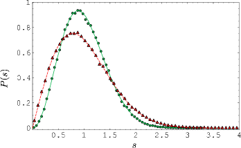
Figure 1: We show the probability density for the nearest neighbor spacing for 18 qubits and averaged over the different relevant $\mathcal{H}_{k}$ spaces ($k=1,\dots,8$). Numerical results are shown in green circles for the model corresponding to the GUE and red triangles for the GOE. Parameters are $M=2$, $b^{(1)}=(1,1,0)$, and $b^{(2)}=(1.4,0,1.4)$ for the GUE case and $b^{(1)}=(1.4,1.4,0)$, for the GOE case. We plot the exact RMT result for both the GOE (dashed red line) and the GUE (continuous green line) since comparison with Wigner surmise is not satisfactory.

We next introduce the multiply kicked Ising model (MKI) as a modification of the kicked Ising model introduced in Prosen (2002). The evolution operator corresponding to one time step is

$$U_{\text{MKI}}=\prod_{n=1}^{M}U_{\text{Ising}}U_{\text{kick}}^{(n)}$$ (9)

with

$$U_{\text{Ising}} =\exp\left(-\imath J\sum_{j=0}^{L-1}\sigma^{z}_{j}\sigma^{z}_{j+1}\right),$$ (10)

$$U_{\text{kick}}^{(n)} =\exp\left(-\imath\sum_{j=0}^{L-1}\vec{b}^{(n)}\cdot\vec{\sigma}_{j}\right),$$ (11)

and periodic boundary conditions $\sigma_{L}\equiv\sigma_{0}$. Here $\sigma^{x,y,z}_{j}$ are the Pauli matrices corresponding to spin 1/2 at position $j$, and $\vec{\sigma}_{j}=(\sigma^{x}_{j},\sigma^{y}_{j},\sigma^{z}_{j})$. The system defined in Eq.(9) represents a periodic 1-d array of $L$ spin $1/2$ particles which periodically receive a sequence of $M$ different kicks of instantaneous magnetic field pulses equally spaced in time. The free evolution ($U_{\text{Ising}}$) is simply given by the Ising interaction between nearest neighbors, with dimensionless strength $J$ which we fix to 1 in the numerical simulations. Each of the $M$ kicks is an instantaneous and homogeneous magnetic field characterized by the dimensionless vector $\vec{b}^{(n)}$. Due to the two body interaction of the system, we are able to evaluate efficiently the evolution of any state Prosen (2002), and hence, as noted in Ketzmerick et al. (1999), also its spectrum. In the previous model Prosen (2002) the same kick was applied periodically, that is $M=1$.

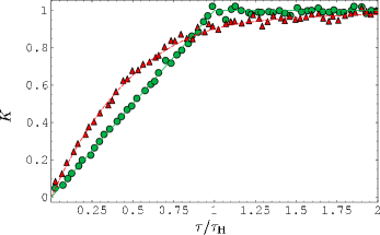
Figure 2: Same parameters and sign conventions as in Fig. 1. We show the spectral form factor averaged over all relevant $\mathcal{H}_{k}$’s. In order to smooth the function, we also average over a window in $t$ of size $0.15t_{\text{H}}$.

Since we wish to compare the behavior of fidelity in our model-system with the average behavior of an ensemble of random matrices, it is necessary to identify the correct symmetry class. To this end, we have to study the symmetries of the MKI model. As couplings between neighboring qubits as well as the effect of the kick on all qubits are equal, it is easy to see that we formally have a ring of qubits and thus a rotational as well as a reflection symmetry.

Let us define the rotational operator $\hat{R}$ over the elements of the computational basis, as $\hat{R}|i_{0}i_{1}\dots i_{L-1}\rangle=|i_{L-1}i_{0}\dots i_{L-2}\rangle$, where each $i_{j}\in\{0,1\}$, and extend it to the other elements of the Hilbert space, requiring linearity. If we visualize our model as a ring, the action of this operator is to rotate the particles in the ring by one position. This operator defines a rotation group ${\cal C}_{L}$. We can further define the reflection operator $\hat{P}$ on the computational basis as $\hat{P}|i_{0}i_{1}\dots i_{L-1}\rangle=|i_{L-1}i_{L-2}\dots i_{0}\rangle$ and again extend it to the whole space requiring linearity. The two operators do not commute and form the group ${\cal C}_{L,v}$ of rotations and reflections of a ring of $L$ elements. Note that the $[U_{\textrm{M}KI},\hat{P}]=[U_{\textrm{M}KI},\hat{R}]=0$, hence the eigenvalues, $\exp(2\pi\imath k/L)$ with $k\in\mathbb{Z}/L$, of the rotation operator define the invariant subspaces which are degenerate with two parities except for the cases $k=0$ and $k=L/2$ the latter for even $L$ only. In the latter cases invariant subspaces of well defined parity can be defined depending on the behavior under reflections, though for a given set of qubits not necessarily both parities need occur. The dimension for any set with fixed $k$ is approximately equal to $2^{L}/L$.

Since we do not identify other symmetries in the system, we expect to find a range of parameters in which each of the blocks of $U_{\text{MKI}}$ corresponding to the minimal invariant subspaces, behave as a typical member of the GUE. This was numerically checked by analyzing the spectra in each of the invariant subspaces, for the parameters shown in the caption of Fig. 1. The resulting nearest neighbor statistics and spectral form factors (both defined in Mehta (1991)) are presented in Fig. 1 and Fig. 2, respectively. Other statistical tests like the number variance, skewness and excess were also applied with excellent agreement with the expected behavior (not shown). The success of these tests is a strong indicator that indeed no other symmetries are present.

Consider now the case in which we have only one periodic kick, that is $M=1$ in $U_{\text{MKI}}$. Rotating each individual spin, the magnetic field ($\vec{b}^{(1)}$) can be made to have only components in the $xz$ plane. The Hamiltonian will have only real components in the basis in which $\sigma^{x,z}_{j}$ are real, hence an anti-unitary symmetry becomes evident. This symmetry $\mathcal{K}$ (complex conjugation in the basis mentioned above) is not time reversal, since spin is being reflected in the $xz$ plane of each qubit, instead of being reversed. Furthermore, this symmetry will change the sign of $k$ and hence, by itself, will not provide an anti-unitary symmetry within the invariant subspaces. Recalling that $\hat{P}$ also reverses the sign of $k$, we observe that the combined operator $\hat{P}\mathcal{K}$, will provide each of the invariant subspaces with an anti-unitary symmetry, which we call time reversal invariance (TRI). We expect then that for $M=1$ the system will have a range of parameters in which each invariant subspace will behave as a typical member of the GOE for some values of the parameters which are sufficiently well separated from the exactly solvable cases of longitudinal and transverse fields Prosen (2000). Numerical evidence favoring this statement is presented in Figs. 1 and 2.

Effectively we will have, for each of the invariant subspaces a Heisenberg time given by $t_{\text{H}}\approx 2^{L}/L$ (the approximate number of levels) except for TRI subspaces for which we shall have $t_{\text{H}}\approx 2^{L-1}/L$.

The perturbation we shall consider is a kick in the $x$ direction:

$$A=\sum_{j=0}^{L-1}\sigma^{x}_{j}$$ (12)

in the Floquet propagator [Eq.(9)]

$$U_{{\rm MKI},\delta}=U_{\rm MKI}\exp(-\imath\delta A).$$ (13)

Comparing the linear response formula for the dynamical model Prosen (2002),

$$f(t)=1-\frac{\delta^{2}}{2}\sum_{t^{\prime}=-t+1}^{t-1}C(t^{\prime})\;,$$ (14)

with the correlation function $C(t)=2^{-L}{\text{Tr}}AU^{\dagger}(t)AU(t)$ with the random matrix model, we connect the perturbation strengths

$$\epsilon=2^{L}\delta^{2}\sigma\;.$$ (15)

Here $\sigma=\lim_{t\to\infty}\lim_{L\to\infty}\frac{1}{2}\sum_{t^{\prime}=-t}^{t}C(t^{\prime})$ is the integrated correlation function of the unperturbed dynamics.

Note that the perturbation will have all the symmetries presented, so that it will not mix the different invariant subspaces. Thus, if we consider an initial state with components from all the $\mathcal{H}_{k}$ spaces, we will obtain an average of fidelity over $L$ different initial conditions each in a different $\mathcal{H}_{k}$ space.

IV Results

Since the effect we want to observe is extremely small, we must have a full understanding of the most important causes of deviation in the evaluation of fidelity in Eq.(6). Note that here we are taking two averages, one of them over the ensemble of Hamiltonians and the other one over the ensemble of initial conditions. The first of this averages we are not going to evaluate in our numerical model since we want to show that an individual quantum chaotic system (in the limit of large Hilbert space dimension) actually behaves according to the random matrix ensemble average over the appropriate symmetry class. The other average (over the Hilbert space) is possible to evaluate in an exact way, taking the average over an orthonormal basis resulting in a trace operation. In practice, for very large Hilbert spaces this method is not efficient. Instead we shall use an approximation which introduces an error that can be made as small as desired.

Figure 3: Different perturbations for the GUE system. We have here 16 qubits and 10 initial conditions. in Fig. 5. Dots show the numerical calculation (real part) and thin curves show RMT prediction whereas red dashed curves show the ELR approximation. We set perturbations to $\epsilon_{1}=5.15$ (in this case all the three curves are overlapping), $\epsilon_{2}=10.3$, $\epsilon_{3}=15.455$, $\epsilon_{4}=20.6$.

Let us first comment on the latter source of error. For any operator $A$, we have that

$${\text{Tr}}A=\left<A\right>_{\psi}\;,$$ (16)

where $\left<\cdot\right>_{\psi}$ denotes the average over Gaussian random states: $|\psi\rangle=\sum_{i=1}^{N}x_{i}|i\rangle$, where $\{|i\rangle\}_{i=1,\dots,N}$ is an orthonormal basis and $x_{i}$ are independent complex Gaussian distributed random numbers with standard deviation $1/\sqrt{N}$. Then, we have that

$${\text{Tr}}A\approx\frac{1}{m}\sum_{j=1}^{m}\left<\psi_{j}|A|\psi_{j}\right>.$$ (17)

Of course letting $m\to\infty$ will make the average exact. But for large $N$ it turns out that already taking a small number of states is enough to have a very good approximation of the expected value of $A$. So we shall evaluate Eq. (6) with the aid of Eq. (17). In particular for the sizes of the Hilbert spaces considered here (upto $2^{20}$) the number of states needed to achieve the precision required is much smaller than the dimension of the space. In our case we want to evaluate the expectation value of the echo operator

$$M_{t}=U_{\delta}^{\dagger}(t)U(t)$$ (18)

for different values of $t$. For a fixed value of $t$ we have a distribution of values of $\left<\psi|M_{t}|\psi\right>$ and hence an associated standard deviation. Although at $t=0$ this standard deviation is zero, after a transient time it approaches an stationary value, determined by finite size effects. We shall call this value $\sigma_{\textrm{finite average}}$. Then the error in the evaluation of ${\text{Tr}}M_{t}$ will be $\sigma_{\textrm{finite average}}/\sqrt{m}$ if we take $m$ sample states. Estimating numerically this value is trivial since for $m$ different realizations we can evaluate the standard deviation at each time and then average over time, for $t$’s larger than the transient time.

Considering only one particular Hamiltonian will also cause some deviations from the exact RMT formula: recall that to obtain, say Eq.(7), we averaged over an ensemble of Hamiltonians. Even if we obtain the exact trace of the echo operator its value will fluctuate in time around the ensemble averaged value. These fluctuations can be characterized with a standard deviation $\sigma_{\textrm{intrinsic}}$. For a fixed Hamiltonian the only way to decrease this number is to increase the dimension of the system. In practice, for computational reasons, we can only achieve results for up to 20 qubits for times of the order of Heisenberg time.

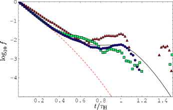
Figure 4: Different number of qubits for a same effective perturbation for the GUE system. The perturbation strength is $\epsilon=20$. We vary the number of qubits, red triangles being 10, green squares 12, and blue circles 16. We have, in all cases, 200 initial conditions. We only show the points where $\textrm{Re}f>0$. The red dashed line is the ELR prediction.

Since those two effects can be assumed to be completely independent, the total average deviation of Eq.(6) will be given by

$$\sigma_{\textrm{total}}^{2}=\sigma_{\textrm{intrinsic}}^{2}+\frac{\sigma_{\textrm{finite average}}^{2}}{m}.$$ (19)

We can estimate a posteriori this quantity very easily, since we know that the imaginary part of the ensemble averaged fidelity amplitude is zero for all times: $\textrm{Im}f(t)=0$. Hence computing the fluctuations of the imaginary part of the data obtained will give us $\sigma_{\textrm{total}}$ and hence $\sigma_{\textrm{intrinsic}}$ (recall that evaluating $\sigma_{\textrm{finite average}}$ is trivial). The knowledge of $\sigma_{\textrm{intrinsic}}$ will give us an estimate for the minimal value of $m$ needed to estimate the value of ${\text{Tr}}M_{t}$ with sufficient accuracy. In the results shown in this section, we always have $\sigma_{\textrm{finite average}}/\sqrt{m}\ll\sigma_{\textrm{intrinsic}}$.

We now turn our attention to the numerical results obtained. We shall set $\vec{b}^{(1)}=(1.4,1.4,0)$. For the GOE case ($M=1$) we do not need to specify any other parameter except for the number of qubits and the strength of the perturbation. The resulting value of the integrated correlation function is found to be $\sigma\approx 1.27$. In case we want to observe the GUE prediction we set $M=2$, take the same $\vec{b}^{(1)}$ as in GOE case and $\vec{b}^{(2)}=(1,0,1)$. The integrated correlation function is found to be $\sigma\approx 0.93$.

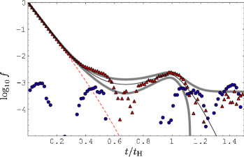
Figure 5: Revival for 20 qubits. The perturbation strength is $\epsilon=31.78$. The red triangles indicate the real part, whereas the blue circles indicate the imaginary part (whenever they are greater than 0), in time steps of 525, calculated with 15 initial conditions. The black thin curve is the RMT theoretical prediction, the red dashed line is the ELR prediction and the gray curves indicate the RMT curve plus/minus the calculated intrinsic deviation.

In Fig. 3 we show, for the GUE-type system, how varying the perturbation parameter changes the behavior of fidelity. Even for fairly large perturbations ($\epsilon_{1}=5.15$) we obtain a fairly good approximation with ELR, which almost coincides with the exact RMT result. For larger perturbations, deviation of the ELR from exact RMT are big enough to be observed, and indeed they are observed clearly for $\epsilon_{1}=10.3$. For $\epsilon_{4}=20.6$, where we should observe a recovery, the behavior at those low fidelities is shadowed by the intrinsic error. Here we chose sufficiently many initial conditions, so that the finite average error is considerably smaller than the intrinsic error.

In Fig. 4 we show, again for the GUE-type system, how increasing the number of qubits decreases the deviation from RMT prediction. We fix the effective perturbation [which scales with the number of qubits as shown in Eq.(15)] and observe the behavior of the real part of fidelity for 10, 12 and 16 qubits. Particularly for 10 qubits we see a noticeable deviation, probably due to the non-vanishing correlation function for large times. This value becomes smaller as the number of qubits increases but also we average over a larger number of invariant subspaces. In all cases we can see that the correspondence with exact RMT is much better than with ELR.

In Fig. 5 we show the evolution of fidelity, for $\epsilon=31.78$ where the revival is strongest. The error due to finite averaging is much smaller than the intrinsic error. We cannot diminish intrinsic error further, since for 20 qubits we need near more than two weeks of computer time per initial condition, and in order to increase the system size by one qubit we need 4 times more CPU time for each initial condition, since for each time step we roughly need to double the number of operations and we also need to double the number of time steps (due to the increase in the Heisenberg time). We expect that for sufficiently large Hilbert spaces the intrinsic error will be so small and the self averaging so strong that even for one initial condition one can clearly observe the fidelity revival.

Finally, for completeness, we also show the behavior for the GOE-type system in Fig. 6. The deviation with ELR is evident, and the error is within the bounds.

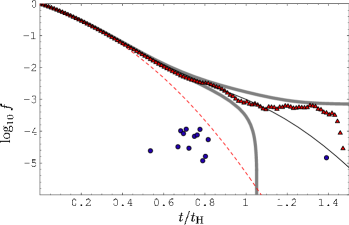
Figure 6: We show that our GOE system indeed behaves as given by the RMT theory. Same color coding as in Fig. 5. The perturbation strength is $\epsilon=10$, and the number of initial conditions is 15. The size of the system is 20 qubits, $h_{\perp}=h_{\parallel}=1.4$. We show only the points where $f>0$. The red dashed line is the ELR prediction.

V Conclusions

The recent exact solutions of the random matrix model for fidelity decay display quite unexpected characteristics for large perturbations and large times. The most remarkable one is the maximum that develops at Heisenberg time. We showed that this phenomenon, established for an ensemble average, can actually be seen in individual dynamical systems if the Hilbert space is large enough: the effect is not overshadowed by noise and finite size effects. Self-averaging is effective, and indeed we find good agreement with RMT results for fidelity decay for two individual kicked spin chain models, one with, one without a pseudo time reversal invariance. The results are achieved without any fit parameter as the perturbation strength has been determined directly from the model we use.

The model used was a kicked spin chain which can reproduce both TRI conserving and TRI breaking dynamics. It has no obvious classical analogue, so we could feel reasonably confident that it would display generic behavior in a regime far from the perturbative one. Whether the maximum at Heisenberg time can also be expected for systems with a classical analog is an open and interesting question. Clearly, for strong perturbations and short times they should not follow RMT behavior, but that does not exclude, that this behavior is recovered at least qualitatively for times as long as the Heisenberg time.