Non locality and causal evolution in QFT

Abstract

Non locality appearing in QFT during the free evolution of localized field states and in the Feynman propagator function is analyzed. It is shown to be connected to the initial non local properties present at the level of quantum states and then it does not imply a violation of Einstein’s causality. Then it is investigated a simple QFT system with interaction, consisting of a classical source coupled linearly to a quantum scalar field, that is exactly solved. The expression for the time evolution of the state describing the system is given. The expectation value of any arbitrary “good” local observable, expressed as a function of the field operator and its space and time derivatives, is obtained explicitly at all order in the field-matter coupling constant. These expectation values have a source dependent part that is shown to be always causally retarded, while the non local contributions are source independent and related to the non local properties of zero point vacuum fluctuations.

†  ‡

1 Introduction

In non relativistic Quantum Electrodynamics (QED) non locality has initially been studied in the context of the energy transfer between couple of atoms, the so-called Fermi problem [1], and then in other systems [2, 3, 4, 5] giving rise to controversial interpretations [6, 7, 8, 9, 10, 11, 12]. In relativistic quantum mechanics Hegerfeldt’s theorem (HT)[13] associates the appearance of non locality to the condition of positivity of the energy. In fact wavefunctions initially localized in finite space regions develop with time non zero contributions and also finite expectation values for some localization operators [14, 15] at spacelike distances from the localization region, apparently at variance with Einstein’s causality.

The use of localization or of position operators to determine if the appearance of non locality gives rise to observable effects appears, however, in relativistic quantum mechanics beset with difficulties[16, 17]. In Quantum Field Theory (QFT), where non local quantities as the Feynman propagator already show up for free fields [6], the standard QFT techniques for interacting fields relate causality to the analytic and unitary properties of the S-matrix [18]. This, with the use of perturbation theory, makes the analysis of causality a “difficult thing in QFT” [19]. In fact the most natural approach to analyze the consequences of HT would be to follow the time development of the systems as is usually done, within perturbation theory, in non relativistic QED. There however other kind of difficulties appears in the description of the sources or the detectors of the field that propagates. These are atoms that to be approximated as effectively point like must be initially described by bare states (that allow structure localized in small space regions) if instead described by dressed states they are inevitably complex structures of atoms plus field extended in space [3, 20, 21]. Another limitation is that here again the analysis can be limited to the lowest orders of perturbation theory.

To overcome some of these difficulties, explicit simplified interacting QFT models with classical sources have been used [2, 4, 9].These permit to follow in detail the time evolution, are not beset with the problems in the definition of the initial states used to describe the sources and cab be solved non perturbatively [4]. In one of these models, consisting of the electromagnetic field interacting with a classical source, it has been shown that while the expectation value of the field energy density behaves causally non local effects appear at the level of quantum states, giving “acausal” effects that are not however “observable” at a classical level [2]. In another model, of a scalar field interacting with a classical instantaneous and point like source and within second order perturbation theory, it has been shown that the evolution of one- and two-point field operators are non local. Non locality however appears either in source independent terms, and may be attributed to zero point vacuum fluctuations, or in source dependent terms and may then be attributed to the use of operators whose commutator is not zero for space like distances and that, not satisfying the microcausality principle, cannot be considered ““good” operators [9].

Because, for a given model, a proof of causality would be required to held at any order and for any “good” local observable, the aim of this paper is to extend the previous perturbative results [9] to all orders and to explicitly calculate the form of the expectation value of any “good” operator, expressed locally in terms of the fields, generalizing the results of references [2] and [4]. Moreover we want also that our analysis of the causality be independent of a specific assigned evolution of the source. For this purpose in the following we shall consider the QFT model of a quantum scalar field linearly interacting with a classical scalar source arbitrarily extended in space and varying in time although localized in an finite space-time region. We aim also to show that the appearance of non locality already at the level of the free field in QFT theory may be attributabed to the fact that, to create localized states, the operators are used that do not create effectively point like states. The paper is structured as follows: in Sec.2 the appearance of non locality for a free quantum scalar field is analyzed. In Sec. 3 and 4 the time evolution of the state of the scalar field coupled to a source and the expectation value on it of arbitrary local “good” operators is obtained. Finally in Sec. 5 we shall comment the results obtained.

2 Single particle amplitude evolution

Locality for quantum fields interacting with source has been investigated by analyzing the expectation values of relativistic localization operators [2, 3, 20]. Here we want to contend that non locality that appears in these treatments may be held to have the same origin of the non local characteristic shown by the standard two-point functions and by the single particle amplitude that already shows up in the free field case. In particular we shall analyze the case of quantum scalar field $\Phi(x)$, $x\equiv(\textbf{x},x^{0}=t)$, that expressed in terms of its positive and negative frequency part is:

$$\Phi(x)=\Phi_{+}(x)+\Phi_{-}(x)$$ (1)

where, taking $\hbar=1$ and $c=1$,

$$\Phi_{+}(x)=\frac{1}{(2\pi)^{3/2}}\int\frac{\rmd^{3}\textbf{k}}{2\omega}\,a(\textbf{k})e^{-ik\cdot x}\quad\textrm{and}\quad\Phi_{-}(x)=\Phi_{+}^{{\dagger}}(x),$$ (2)

with $\omega=\sqrt{|\textbf{k}|^{2}+m^{2}}$ and $a(\textbf{k})$, $a^{{\dagger}}(\textbf{k})$ being respectively the usual annihilation and creation operators that satisfy the relativistic commutator rules:

$$\left[a(\textbf{k}),a^{{\dagger}}(\textbf{k}^{\prime})\right]=2\omega\delta^{3}(\textbf{k}-\textbf{k}^{\prime}).$$ (3)

The state $\Phi(x)|0\rangle$ generated by the action of the field operator on the vacuum field state $|0\rangle$, using equations (1) and (2), is

$$\Phi(x)|0\rangle=\Phi_{-}(x)|0\rangle=\frac{1}{(2\pi)^{3/2}}\int\frac{\rmd^{3}\textbf{k}}{2\omega}\,e^{ik\cdot x}\,a^{{\dagger}}(\textbf{k})|0\rangle$$ (4)

where $\Phi_{+}(x)|0\rangle=0$ has been taken into account. $\Phi(x)|0\rangle$ is a linear superposition of single particle states $a^{{\dagger}}(\textbf{k})|0\rangle=|\textbf{k}\rangle$, eigenstates of the momentum operator with eigenvalue k. Except for the factor $1/2\omega$, expression (4) corresponds to the non relativistic expansion in terms of momenta of the eingenstate position $|\textbf{x}\rangle$. Thus one is lead to assume [22] that $\Phi(x)|0\rangle$ represents the “localized” state where a single particle is created at position x. Apparently a confirmation is given by the fact that projecting this state on momentum eigenstate $|\textbf{k}\rangle$, we obtain

$$\langle 0|\Phi(x)|\textbf{k}\rangle=\frac{1}{(2\pi)^{3/2}}\int\frac{\rmd^{3}\textbf{k}^{\prime}}{2\omega}\,e^{-ik^{\prime}\cdot x}\,\langle 0|a(\textbf{k}^{\prime})a^{{\dagger}}(\textbf{k})|0\rangle=\frac{e^{-ik\cdot x}}{(2\pi)^{3/2}}$$ (5)

and thus interpret the above expression as the space representation of the single particle wavefunction of the state $|\textbf{k}\rangle$, just as in non relativistic quantum mechanics $\langle\textbf{x}|\textbf{k}\rangle\propto e^{-ik\cdot x}$ is the wavefunction of $|\textbf{k}\rangle$. However as we shall see this interpretation cannot be held too strictly. In fact the two-point function given by the scalar product between $\Phi(x)|0\rangle$ and $\Phi(y)|0\rangle$ is:

$$\langle 0|\Phi(x)\Phi(y)|0\rangle=\frac{1}{(2\pi)^{3}}\int\frac{\rmd^{3}\textbf{k}}{2\omega}\,e^{-ik\cdot(x-y)}=i\Delta_{+}(x-y)$$ (6)

where $\Delta_{+}(x-y)$ is the positive frequency propagator part of $\Delta$ function. Equation (6) is interpreted as the probability amplitude of finding at spacetime point $y$ a particle created at point $x$. The explicit form of $\Delta_{+}(x-y)$ [22, 23] shows that it is not zero for $x-y$ spacelike and does not tend to $3$-dimension $\delta$ function when $x_{0}\rightarrow y_{0}$. In fact:

$$\lim_{x_{0}\rightarrow y_{0},|x-y|\rightarrow\infty}\Delta_{+}(x-y)\propto\left\{\begin{array}[]{ccc}e^{-m|x-y|}&\quad\textrm{for}\quad m\neq 0\\ \frac{1}{|x-y|^{2}}&\quad\textrm{for}\quad m=0\end{array}\right..$$ (7)

Considering instead the equation (6) as the scalar product of the the states $\Phi(x)|0\rangle$ and $\Phi(y)|0\rangle$, describing a single particle localized respectively at spacetime points $x$ and $y$, we see a spatial overlap for spacelike distances. This peculiar behaviour can be avoided if we give up the interpretation of $\Phi(x)|0\rangle$ as a state where a particle is created in x and is there $\delta$ like localized, but instead that is represents a state, extending over the whole space, centered at x. This interpretation is also supported by evaluating on this state “good” local observables that satisfy the microcausality principle. In particular taking the scalar field energy density at $x$:

$$\!\mathcal{H}(x)\!=\!\frac{1}{2}\!\left(\!|\nabla\Phi(x)|^{2}\!\!+\!\dot{\Phi}(x)^{2}\!+\!m^{2}\Phi^{2}(x)\!\right)$$ (8)

it has the expectation value on the “localized” state at $y$ $\Phi(y)|0\rangle$

$$\langle 0|\Phi(y)\mathcal{H}(x)\Phi(y)|0\rangle\!=-2m^{2}\Delta_{+}(x-y)\Delta_{+}(y-x)$$

$$-2\partial_{x_{0}}\Big{(}\Delta_{+}(x-y)\Delta_{+}(y-x)\Big{)}-2\nabla_{x}\Big{(}\Delta_{+}(x-y)\Delta_{+}(y-x)\Big{)}{}$$

$$-\lim_{s\rightarrow 0}\Big{(}m^{2}\Delta_{+}^{2}(s)+\Delta_{+}(s)\,\partial_{s_{0}}^{2}\Delta_{+}(s)+\Delta_{+}(s)\,\nabla_{s}^{2}\Delta_{+}(s)\Big{)}$$ (9)

which, from the properties of the $\Delta_{+}$ two-point function given by the expression (7), can be seen to have contributions different from zero over the whole space and not a $\delta$ behaviour.

This interpretation of the state $\Phi(x)|0\rangle$ permits us to explain the appearance of non local effects present in the Feynman propagator $\Delta_{F}$:

$$\Delta_{F}(x-y) = \langle 0|T\{\Phi(x)\Phi(y)\}|0\rangle$$ (10)

$$= \Theta(x_{0}-y_{0})\langle 0|\Phi(x)\Phi(y)|0\rangle+\Theta(y_{0}-x_{0})\langle 0|\Phi(y)\Phi(x)|0\rangle,$$

$T$ being the time ordering operator, with each of the terms appearing in the equation (10) is usually considered as the amplitude probability of propagation of particles localized from $y$ to $x$ (or vice versa). Following our previous discussion one can interpret it as the amplitude of going from the non localized state centered at y to the corresponding centered at $x$. It may therefore be expected, because these states are extended in space, that the overlap among these may be non zero also for $|x-y|$ spacelike.

It may also be of interest to verify if the one particle states $\Phi(x)|0\rangle$, on which the local expectation value of the field energy density is non local, may instead satisfy the relativistic notion of localization adopted in relativistic quantum mechanics. In this framework the second quantized position operator $\textbf{x}=i\nabla_{\textrm{\scriptsize{k}}}$ is not anymore hermitian and this has lead to introduce new definition for the position operator and the states localized at a given position [2, 3, 20]. In particular the Newton-Wigner (NW) localized states are single particle states obtained when the “localization” creation operator $a_{NW}^{{\dagger}}(x)$ acts on vacuum state $|0\rangle$ [24, 25]. This operator is related to the negative frequency part of the field operator $\Phi(x)$ by a non local integral transformation [25]:

$$a_{NW}^{{\dagger}}(x)=\int d^{3}\textbf{x}^{\prime}K_{NW}(|\textbf{x}-\textbf{x}^{\prime}|)\Phi_{-}(\textbf{x}^{\prime},x_{0})$$ (11)

where the Kernel $K_{NW}$ defined as

$$K_{NW}(mR)=\frac{1}{(2\pi)^{3}}\int d^{3}\textbf{k}\sqrt{2\omega}\,e^{i\textbf{\scriptsize{k}}\cdot\textbf{\scriptsize{R}}}$$ (12)

has this asymptotic behaviour when $R$ tends to infinity

$$\lim_{R\rightarrow\infty}{K_{NW}}(R)\rightarrow\left\{\begin{array}[]{ccc}cost\frac{m^{7/2}}{(mR)^{9/4}}e^{-mR},&\quad\textrm{for}\quad m\neq 0\\ &\\ costR^{-7/2},&\quad\textrm{for}\quad m\neq 0\end{array}\right..$$ (13)

Thus $K_{NW}$ extends, for massive fields ($m\neq 0$), in a space region of dimension comparable to Compton wavelength $1/m$, while for massless fields $m=0$ it decreases for large distance with the power law. In this context the NW state localized at x at time $x_{0}$ is written as

$$|X_{NW}\rangle=a_{NW}^{{\dagger}}(x)|0\rangle=\frac{1}{(2\pi)^{3/2}}\int\frac{d^{3}\textbf{k}}{\sqrt{2\omega}}\,\,a^{{\dagger}}(\textbf{k})|0\rangle$$ (14)

and its scalar product with a NW state localized at y at $x_{0}=y_{0}$ may be shown to be:

$$\langle X_{NW}|Y_{NW}\rangle=\delta^{3}(\textbf{x}-\textbf{y})\quad\textrm{for}$$ (15)

therefore satisfying the standard non relativistic condition for a $\delta$ localized state. To examine if the state, created from vacuum by the field operator, $\Phi(x)|0\rangle$ may be considered localized in NW sense, we take its scalar product with state $|Y_{NW}\rangle$ obtaining:

$$\langle 0|\Phi(x)|Y_{NW}\rangle = i\int d^{3}\textbf{x}^{\prime}K_{NW}(m|\textbf{y}-\textbf{x}^{\prime}|)\Delta_{+}(x-x^{\prime}){}$$ (16)

$$= \frac{1}{(2\pi)^{3}}\int\frac{d^{3}\textbf{k}}{\sqrt{2\omega}}e^{-ik\cdot(x-y)}=\psi_{y}^{NW}(x)$$

where interestingly $\psi_{y}^{NW}(x)$ is just the NW expression for first quantized relativistic state localized at y, which differs from zero for $(x-y)$ spacelike and does not reduce to $3$-dimension $\delta$ function even for $x_{0}=y_{0}$. Thus the state $\Phi(x)|0\rangle$ cannot be even considered localized in the NW sense. This is another indication that one particle states created from vacuum by a direct application of the field operator cannot represent physical situations with the single particle restricted to an arbitrarily small region of space.

As known the use of NW localized states leads with time to the appearance of non local terms. In fact the scalar product of the NW state localized at y at $x_{0}>y_{0}$ when projected on the NW state localized at x at $x_{0}$ is

$$\langle X_{NW}|Y_{NW}\rangle=-2\partial_{x_{0}}\Delta_{+}(x-y)\neq\delta^{3}(\textbf{x}-\textbf{y})$$ (17)

differing from zero for spacelike distances. So a single particle state initially NW localized spreads non causally with time and this result can be interpreted as an example of the HT.

3 The QFT model with source

In the previous section we have seen that in QFT non locality shows up at the level of single particle states and of transition amplitude because the action of the free field operator $\Phi(x)$ on the vacuum effectively generates non local states. It seems relevant to inquire if this non local behaviour may be observed and this leads to consider situations where the the field quantities are generated and detected. To this purpose we shall explicitly examine the case of a quantum scalar field $\Phi(x)$ linearly interacting with a classical time dependent source $j(x)$ [2, 9]. This choice permits to localize the source within an arbitrary region of spacetime avoiding the problems of locality connected to the use of bare or dressed state in its quantum description [4]. The Hamiltonian describing the system is then:

$$H_{tot}=H_{0}+H_{int}$$ (18)

with

$$H_{0} = \frac{1}{2}\int\frac{\rmd^{3}\textbf{k}}{2\omega}\,\omega\left(a^{{\dagger}}(\textbf{k})a(\textbf{k})+a(\textbf{k})a^{{\dagger}}(\textbf{k})\right)$$

$$H_{int} = g\int_{-\infty}^{+\infty}\rmd^{3}\textbf{x}\Phi(x)j(x)$$ (19)

where $g$ is the source-field coupling constant. In this model the time evolution of the source is assigned and the quantum aspects of the system are described by the field quantum state. The equation of motion, in the interaction picture, is

$$i\frac{\partial}{\partial t}|t\rangle=H_{int}|t\rangle.$$ (20)

By taking as initial condition at $t=0$ the source off $\big{(}j(\textbf{x},0)=0\big{)}$ and the field in its vacuum state $|0\rangle$, the formal solution of the equation (20) is:

$$|t\rangle=U(t)|0\rangle$$ (21)

where time evolution operator is:

$$U(t)=T\exp\left(-i\int_{0}^{t}\rmd t^{\prime}H_{int}(t^{\prime})\right)$$ (22)

with $T$ the time ordering operator. In our model the commutator of the interaction of Hamiltonian at two different times is a c-number given by:

$$[H_{int}(t_{1}),H_{int}(t_{2})]=ig^{2}\int\rmd^{3}\textbf{x}_{1}\int\rmd^{3}\textbf{x}_{2}\Delta(\textbf{x}_{1}-\textbf{x}_{2},t_{1}-t_{2})j(\textbf{x}_{1},t_{1})j(\textbf{x}_{2},t_{2})$$ (23)

where the propagator $\Delta$ function is given in terms of the field commutator as [23]:

$$[\Phi(x),\Phi(y)]=i\Delta(x-y).$$ (24)

$\Delta(x)$ is real and is zero when its argument is spacelike ($x^{2}<0$). This allows [26] to write the $U(t)$ as

$$U(t)=\exp\left(-i\int_{0}^{t}\rmd t^{\prime}H_{int}(t^{\prime})\right)e^{-\xi(t)}$$ (25)

where

$$\xi(t)=\frac{1}{2}\int_{0}^{t}\rmd t_{1}\int_{0}^{t}\rmd t_{2}[H_{int}(t_{1}),H_{int}(t_{2})]\Theta(t_{1}-t_{2}){}$$ (26)

$$=\frac{ig^{2}}{2}\int_{0}^{t}\!\!\rmd t_{1}\int_{0}^{t}\!\!\rmd t_{2}{}$$

$$\times\int\!\!\rmd^{3}\textbf{x}_{1}\int\!\!\rmd^{3}\textbf{x}_{2}\Delta(\textbf{x}_{1}-\textbf{x}_{2},t_{1}-t_{2})j(\textbf{x}_{1},t_{1})j(\textbf{x}_{2},t_{2})\Theta(t_{1}-t_{2}).$$

Because $\Delta(x)$ and $j(x)$ are real, $\xi(t)$ given by the expression (25) is an ordinary imaginary function.

By using the decomposition of the field $\Phi(x)$ in terms of its positive and negative frequency parts, as given in equation (1), it is possible to transform the evolution operator $U(t)$ in the form [26]:

$$U(t)=\exp\left(-i\int_{0}^{t}\rmd t^{\prime}H_{int}^{-}(t^{\prime})\right)\exp\left(-i\int_{0}^{t}\rmd t^{\prime}H_{int}^{+}(t^{\prime})\right)e^{-\xi(t)}e^{\alpha(t)}$$ (27)

where

$$H_{int}^{\pm}(t)=g\int\rmd^{3}\textbf{x}\Phi_{\pm}(\textbf{x},t)j(\textbf{x},t)$$ (28)

and

$$\alpha(t) = -\frac{1}{2}\Bigg{[}-i\int_{0}^{t}\rmd t^{\prime}H_{int}^{-}(t^{\prime}),-i\int_{0}^{t}\rmd t^{\prime\prime}H_{int}^{+}(t^{\prime\prime})\Bigg{]}$$ (29)

$$= \frac{ig^{2}}{2}\int_{0}^{t}\rmd t_{1}\int_{0}^{t}\rmd t_{2}\int\rmd^{3}\textbf{x}_{1}\int\rmd^{3}\textbf{x}_{2}j(\textbf{x}_{1},t_{1})\Delta_{-}(\textbf{x}_{1}-\textbf{x}_{2},t_{1}-t_{2})j(\textbf{x}_{2},t_{2})$$

where $\Delta_{-}$ is the negative frequency part of the propagator $\Delta$ given by

$$[\Phi_{-}(x),\Phi_{+}(y)]=i\Delta_{-}(x-y).$$ (30)

The exponent $\alpha(t)$ in the expression (27) is an ordinary function and the equation (29) gives its dependence from the source $j(x)$. The form (29) of the evolution operator makes possible to obtain simply the time evolution from any initial state. In fact with our initial condition the equations (21) and (27) give the state of the system as:

$$|t\rangle=U(t)|0\rangle=e^{\alpha(t)}e^{-\xi(t)}\exp\left(-i\int_{0}^{t}\rmd t^{\prime}H_{int}^{-}(t^{\prime})\right)|0\rangle$$ (31)

where use has been made of the fact that $H_{int}^{+}(t^{\prime})$ contains only annihilation operators. The state $|t\rangle$ is not a single particle state, however its single particle component can be shown to behave non locally as was the case of the single particle state generated previously by the application of the free field operator on the vacuum. In fact projecting the state $|t\rangle$ on the one-particle quantum state $|\textbf{x}\rangle=a^{{\dagger}}(\textbf{x})|0\rangle$ we get the single particle amplitude transition $\psi(x)$:

$$\psi(x)=\langle 0|a(\textbf{x})|t\rangle = g\int_{0}^{t}\rmd t^{\prime}\int\rmd^{3}\textbf{x}^{\prime}j(\textbf{x}^{\prime},t^{\prime})\Delta_{+}(\textbf{x}-\textbf{x}^{\prime},t-t^{\prime})$$ (32)

$$= g\int_{0}^{t}\rmd t^{\prime}\int\rmd^{3}\textbf{x}^{\prime}j(\textbf{x}^{\prime},t^{\prime})\langle 0|\Phi(x)\Phi(x^{\prime})|0\rangle.$$

From the properties of $\Delta_{+}$ it is immediate to deduce from the expression (32) that the single particle amplitude probability in the case of the state generated from the source develops non zero contribution outside the light cone. This behaviour is connected to the corresponding one of the free field transition amplitude given by the equation (6). This result is again in agreement with the Hegerfeldt’s theorem and with previous results on the non local behaviour of relativistic wavefunctions [9, 27].

Moreover we note that expression in equation (32) for the single particle amplitude probability is exact to all order. If the time spacetime region where the source is different from zero is an infinitesimal region around the spacetime point $y=(\textbf{y},y_{0})$, we have $j(x)=\delta^{4}(x-y)$ and substituting in equation (32) we obtain:

$$\psi(x)=g\,\Theta(t-y_{0})\Delta_{+}(\textbf{x}-\textbf{y}^{\prime},t-y_{0}).$$ (33)

This result is identical to the one obtained previously for pointlike sources within the first order of perturbation theory [9].

4 Expectation values of one-point “good operators”

As shown before non local behaviour of single particle amplitudes does not appear to be a good test of non locality in QFT being built from scalar product of spatially extended states or from states whose projection do not satisfy the microcausality principle. In view of the previous considerations it remains the question if non local behaviours can be observed. To give a meaning to this question it is necessary to examine not only the generation but also the other side of the complete process that is the detection. It has been previously shown [9], within second order perturbation theory, that the calculation of averages, on states generated by pointlike sources, of one-point localization operators give results that cannot be interpreted as the presence of non local properties if these operators do not satisfy the microcausality principle [9]. Therefore in the following we shall consider the average values of “good” one-point operators satisfying the microcausality principle and that are expressed in terms of the field operator and its space and time derivatives at a given spacetime point. The result will be exact and valid for any “good” operator.

The adjoint of the time evolution operator $U(t)$ is immediately obtained as:

$$U^{{\dagger}}(t)=U^{-1}(t)=e^{\xi(t)}e^{-\alpha(t)}\exp\left(i\int_{0}^{t}\rmd t^{\prime}H_{int}^{+}(t^{\prime})\right)\exp\left(i\int_{0}^{t}\rmd t^{\prime}H_{int}^{-}(t^{\prime})\right).$$ (34)

At first we shall consider the expectation value of the field operator $\Phi(x)$ on the state generated by the source $|t\rangle$, which is given by:

$$\langle t|\Phi(x)|t\rangle = \langle 0|U^{-1}(t)\Phi(x)U(t)|0\rangle$$ (35)

$$= \langle 0|U^{-1}(t)\left(U(t)\Phi(x)+\left[\Phi(x),U(t)\right]\right)|0\rangle.$$

The commutator appearing above can be transformed, using equations (3) and (27), as

$$[\Phi(x),U(t)] = -iU(t)\int_{0}^{t}\rmd t^{\prime}[\Phi(x),H_{int}(t^{\prime})]$$ (36)

$$= U(t)g\int_{0}^{t}\rmd t^{\prime}\int\rmd^{3}\textbf{x}^{\prime}j(\textbf{x}^{\prime},t^{\prime})\Delta(\textbf{x}-\textbf{x}^{\prime},t-t^{\prime})$$

Thus, taking into account that $\langle 0|\Phi(x)|0\rangle=0$ and introducing the retarded propagator $\Delta^{ret}(x)=\Theta(t)\Delta(x)$, the expectation value (35) takes the form:

$$\langle t|\Phi(x)|t\rangle=g\int_{0}^{t}\rmd t^{\prime}\int\rmd^{3}\textbf{x}^{\prime}j(\textbf{x}^{\prime},t^{\prime})\Delta_{ret}(\textbf{x}-\textbf{x}^{\prime},t-t^{\prime})=g\widetilde{\Delta}_{R}(x-y).$$ (37)

In equation (37) it is $t>t^{\prime}>0$, while $(x-y)\equiv(\textbf{x}-\textbf{y},t-y_{0})$ and (y, $y_{0}$) indicates a spacetime point inside the spacetime region where $j(\textbf{x},t)\neq 0$. Therefore the function $\widetilde{\Delta}_{R}(x-y)$ defined by the expression (37) contains the spacetime evolution of the source and, because of its construction, is zero outside a forward lightcone containing the spacetime region where the source is non zero. This lightcone has a vertex in the part of the spacetime region where $j(\textbf{x},t)=0$ (Figure 1).

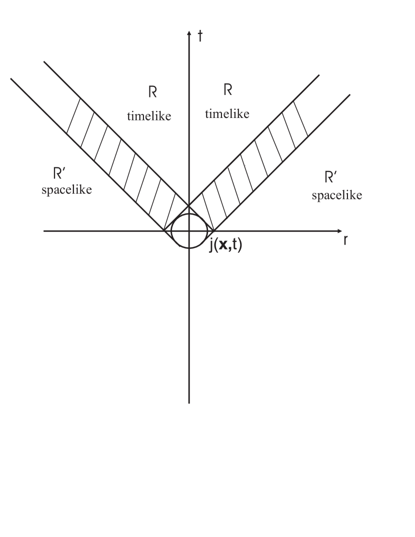
Figure 1: Source forward lightcone: the effects present in separation regions between R and R’ may be local for a part of source and non local for another.

As a consequence of the linearity of the equation of motion of the quantum scalar field, the expression for $\langle\Phi(x)\rangle$ is identical to the retarded solution obtained by a classical scalar field satisfying the equation of motion

$$\left(\frac{\partial^{2}}{\partial t^{2}}-\nabla^{2}+m^{2}\right)\Phi(\textbf{x},t)=g\,j(\textbf{x},t)$$ (38)

where $j(\textbf{x},t)$ is the same source appearing in the quantum equations. For a classical scalar source differing from zero only in an infinitesimal spacetime region around $y=(\textbf{y},y_{0})$, it is $j(x)=\delta^{4}(x-y)$. In this case the equation of motion (37) gives for the average scalar field

$$\langle\Phi(x)\rangle=g\Delta_{ret}(x-y).$$ (39)

This result is exact and corresponds to the one obtained previously within the second order of perturbation theory in the case of pointlike sources [9]. This shows that, at least for the field expectation value, the result obtained via second order perturbation theory is exact.

We shall consider the expectation value of a generic operator $\widehat{O}(x)$ that may be expressed as an arbitrary analytical function of the field operator and of its space and time derivatives. Its expansion in power series being

$$\widehat{O}(\Phi(x),\dot{\Phi}(x),\nabla\Phi(x))=\sum_{j,k,l}c_{jkl}\Phi^{j}(x)\dot{\Phi}^{k}(x)(\nabla\Phi)^{l}(x)$$ (40)

with $c_{j,kl}$ ordinary coefficients. To obtain the average value of $\widehat{O}(x)$ we have to evaluate the expectations value of the powers and products of the field operator and its time and space derivatives.

First we shall consider the expectation value, on the state $|t\rangle$ given by equation (21), of the m-power of the field operator $\Phi^{m}(x)$ . Using the explicit calculation of A we find:

$$\langle t|\Phi^{m}(x)|t\rangle = \langle 0|(g\widetilde{\Delta}_{R}(x-y)+\Phi(x))^{m}|0\rangle$$ (41)

$$= \sum_{\nu=0}^{m}{m\choose\nu}\left(g\widetilde{\Delta}_{R}(x-y)\right)^{\nu}\langle 0|\Phi^{m-\nu}(x)|0\rangle$$

In the expression (41) the first term (for $\nu=0$) $\langle 0|\Phi^{m}(x)|0\rangle$ is the only one independent from the field source coupling constant $g$. Moreover it differs from zero over the whole spacetime and it represents the expectation values of $\Phi^{m}(x)$ on the vacuum state. The remaining terms are source dependent and, because of the presence of the term $g\widetilde{\Delta}_{R}(x-y)$, causally retarded. In order to examine the causal effects due to the variation of the source the vacuum contribution must therefore be subtracted in the expression (41) in agreement with previous results [12, 28, 29, 8].

Equation (41) has a simple interpretation: the expectation value of the m-th power of the field operator in our system is equal to the m-th power of the field operator on the vacuum shifted by $g\widetilde{\Delta}_{R}(x-y)$. This result of the expression (41) has been obtained independently from the explicit expression of the initial state of the field and utilizing only relationship between $\Phi^{m}(x)$, the time evolution operator $U(t)$ and its adjoint $U^{{\dagger}}(t)$. Thus the result given by the equation (41) can be extended to:

$$\langle t_{i}|\Phi^{m}(x)|t_{i}\rangle=\langle i|g\widetilde{\Delta}_{R}(x-y)+\Phi(x))^{m}|i\rangle$$ (42)

where now $|i\rangle$ is an arbitrary initial state for the field and $|t_{i}\rangle=U(t)|i\rangle$.

We shall now proceed to calculate the expectation value on our state $|t\rangle$ of the gradient of the field operator $\nabla_{\textbf{\scriptsize{x}}}\Phi(x)$. It is:

$$\langle t|\nabla_{\textbf{\scriptsize{x}}}\Phi(x)|t\rangle = \langle 0|U^{-1}(t)\nabla_{\textbf{\scriptsize{x}}}\Phi(x)U(t)|0\rangle$$ (43)

$$= \langle 0|U^{-1}(t)\left(U(t)\nabla_{\textbf{\scriptsize{x}}}\Phi(x)+\left[\nabla_{\textbf{\scriptsize{x}}}\Phi(x),U(t)\right]\right)|0\rangle.$$

The commutator appearing above can easily obtained by noting that $\nabla_{\textbf{\scriptsize{x}}}$ acts only on space coordinate. Thus using also the equations (36) and (37), we get:

$$\left[\nabla_{\textbf{\scriptsize{x}}}\Phi(x),U(t)\right]=\nabla_{\textbf{\scriptsize{x}}}\left[\Phi(x),U(t)\right]=g\,U(t)\nabla_{\textbf{\scriptsize{x}}}\widetilde{\Delta}_{R}(x-y)$$ (44)

and by substituting this in the expression (43), we obtain at the end:

$$\langle t|\nabla_{\textbf{\scriptsize{x}}}\Phi(x)|t\rangle=g\nabla_{\textbf{\scriptsize{x}}}\widetilde{\Delta}_{R}(x-y)$$ (45)

where use has been made of $\langle 0|\nabla_{\textbf{\scriptsize{x}}}\Phi(x)|0\rangle=0$. The expectation value of $\nabla_{\textbf{\scriptsize{x}}}\Phi(x)$ is thus simply expressed in terms of the gradient $\widetilde{\Delta}_{R}(x-y)$; it is therefore again retarded and causal. The expectation value of the m-th power of $\nabla_{\textbf{\scriptsize{x}}}\Phi(x)$ may be obtained following with the appropriate changes the procedure followed to calculate the expectation value of $\Phi^{m}(x)$. We get in this case:

$$\langle t|(\nabla_{\textbf{\scriptsize{x}}}\Phi(x))^{m}|t\rangle = \langle 0|\left(\nabla_{\textbf{\scriptsize{x}}}\Phi(x)+g\nabla_{\textbf{\scriptsize{x}}}\widetilde{\Delta}_{R}(x-y)\right)^{m}|0\rangle$$ (46)

$$= \sum_{\nu=0}^{m}{m\choose\nu}\left(g\nabla_{\textbf{\scriptsize{x}}}\widetilde{\Delta}_{R}(x-y)\right)^{\nu}\langle 0|(\nabla_{\textbf{\scriptsize{x}}}\Phi(x))^{m-\nu}|0\rangle.$$

As last we proceed to calculate the expectation value of time derivative of the field operator $\partial_{t}\Phi(x)$ and of its m-th power. The expectation value of $\partial_{t}\Phi(x)$ on the state $|t\rangle$ is

$$\langle t|\partial_{t}\Phi(x)|t\rangle = \langle 0|U^{-1}\partial_{t}\Phi(x)U(t)|0\rangle$$ (47)

$$= \langle 0|U^{-1}(t)\left(U(t)\partial_{t}\Phi(x)+\left[\partial_{t}\Phi(x),U(t)\right]\right)|0\rangle.$$

In this case to calculate the commutator appearing in expression (47) use can be made of the equations (3) and (27) obtaining:

$$[\partial_{t}\Phi(x),U(t)] = -iU(t)\int_{0}^{t}\rmd t^{\prime}[\partial_{t}\Phi(x),H_{int}(t^{\prime})]$$ (48)

$$= -iU(t)\Big{\{}\frac{\partial}{\partial t}\Big{(}\int_{0}^{t}\rmd t^{\prime}[\Phi(x),H_{int}(t^{\prime})]\Big{)}-[\Phi(x),H_{int}(t)]\Big{\}}$$

$$= U(t)g\partial_{t}\widetilde{\Delta}_{R}(\textbf{x}-\textbf{y},t-y_{0})$$

where it has been exploited the property that $\Delta(x)$ is zero when its argument is spacelike. Substituting the expression (48) in (47), we get

$$\langle t|\partial_{t}\Phi(x)|t\rangle=g\partial_{t}\widetilde{\Delta}_{R}(x-y)$$ (49)

where $\langle 0|\partial_{t}\Phi(x)|0\rangle=0$ has been taken into account. The expectation value of $\partial_{t}\Phi(x)$ in equation (49) is expressed as time derivative of $\widetilde{\Delta}_{R}(x-y)$ and is thus causally retarded. Similarly to the previous results the expectation value on $|t\rangle$ of $(\partial_{t}\Phi)^{m}(x)$ is:

$$\langle t|(\partial_{t}\Phi)^{m}(x)|t\rangle = \langle 0|(\partial_{t}\Phi(x)+g\partial_{t}\widetilde{\Delta}_{R}(x-y)^{m}|0\rangle$$ (50)

$$= \sum_{\nu=0}^{m}{m\choose\nu}\left(g\partial_{t}\widetilde{\Delta}_{R}(x-y)\right)^{\nu}\langle 0|(\partial_{t}\Phi^{m-\nu}(x)|0\rangle$$

The results obtained in equations (41), (46) and (50) can be used to evaluate the expectation value of the operator $\widehat{O}(\Phi(x),\dot{\Phi}(x),\nabla\Phi(x))$ analytical function of field operator and its derivatives. In particular the average value of a generic term of the power series of equation (40), takes the form

$$\langle t|\Phi^{j}(x)\dot{\Phi}^{k}(x)(\nabla\Phi)^{l}(x)|t\rangle=$$

$$\langle 0|U^{-1}(t)\Phi^{j}(x)U(t)U^{-1}(t)\dot{\Phi}^{k}(x)U(t)U^{-1}(t)(\nabla\Phi)^{l}(x)U(t)|0\rangle=$$

$$\langle 0|\Big{(}\Phi(x)+g\widetilde{\Delta}_{R}(x-y)\Big{)}^{j}\Big{(}\dot{\Phi}(x)+g\partial_{t}\widetilde{\Delta}_{R}(x-y)\Big{)}^{k}\Big{(}\nabla\Phi(x)+g\nabla\widetilde{\Delta}_{R}(x-y)\Big{)}^{l}|0\rangle$$ (51)

In this case we observe that the expectation value, on the field vacuum, of the term appearing in (4), $\langle 0|\Phi^{j}(x)\dot{\Phi}^{k}(x)(\nabla\Phi)^{l}(x)|0\rangle$, is source independent and in general not zero all over the spacetime. All the remaining terms contain at least a factor $g\widetilde{\Delta}_{R}(x-y)$ and its space or time derivative; therefore they depend on the source and are causally retarded. Thus the expectation value of any observable $\widehat{O}(\Phi(x),\dot{\Phi}(x),\nabla\Phi(x))$, that may be expanded as in the expression (40) shows a causal evolution if its expectation value on the field vacuum is subtracted. This result is valid to all orders of the coupling constant and is the main result of this paragraph. It extends for our QFT model the previous results [2, 12, 8, 28, 29] obtained at finite order of perturbation theory.

Using equation (4) the expectation value of the observable $\widehat{O}(\Phi(x),\dot{\Phi}(x),\nabla\Phi(x))$ on $|t\rangle$ may be explicitly written as:

$$\quad\langle t|\widehat{O}(\!\Phi(x),\dot{\Phi}(x),\nabla\Phi)(x)|t\rangle=$$

$$\qquad\langle 0|\widehat{O}\!\left(\!\Phi(x)+g\widetilde{\Delta}_{R}(x-y),\dot{\Phi}(x)+g\partial_{t}\widetilde{\Delta}_{R}(x-y),\nabla\Phi(x)+g\nabla\widetilde{\Delta}_{R}(x-y)\right)\!\!|0\rangle$$ (52)

The above expression is one of the main results of our paper and shows that the expectation value of $\widehat{O}$ on $|t\rangle$ coincides with the expectation value on the field vacuum of the same expression in terms of operator $\Phi(x)$ and its derivative shifted by $g\widetilde{\Delta}_{R}(x-y)$ and its corresponding derivatives.

The above results permit to obtain immediately the explicit form of the expectation value of any arbitrary one-point observable represented as a function of the field operator and its space and time derivatives. In the following we shall apply this result to the energy density of the field defined by the equation (8). Following the above recipes its expectation value on $|t\rangle$ is immediately given by:

$$\langle t|\mathcal{H}(x)|t\rangle = \langle 0|\mathcal{H}(x)|0\rangle$$ (53)

$$+ 1/2\Bigg{(}\Big{(}\partial_{t}{g\widetilde{\Delta}}_{R}(x-y)\Big{)}^{2}+m^{2}\Big{(}g\widetilde{\Delta}_{R}(x-y)\Big{)}^{2}+\Big{|}\nabla_{x}g\widetilde{\Delta}_{R}(x-y)\Big{|}^{2}\Bigg{)}$$

where the expectation values on the vacuum of the field and its derivatives are zero. The first term of expression (53) represents the vacuum contribution to energy density, the second, as expected from the previous discussion, is source dependent and causally retarded. Although the two point correlation function on $|t\rangle$ is not of the form (4) depending on the field at two separate spacetime points, it is also possible to obtain its expectation value on $|t\rangle$ as:

$${}\langle t|\Phi(x)\Phi(x^{\prime})|t\rangle = \langle 0|U^{-1}(t)\Phi(x)U(t)U^{-1}(t)\Phi(x^{\prime})U(t)|0\rangle$$ (54)

$$= \langle 0|\Big{(}\Phi(x)+g\widetilde{\Delta}_{R}(x-y)\Big{)}\Big{(}\Phi(x^{\prime})+g\widetilde{\Delta}_{R}(x^{\prime}-y)\Big{)}|0\rangle$$

$$= \langle 0|\Phi(x)\Phi(x^{\prime})|0\rangle+g^{2}\widetilde{\Delta}_{R}(x-y)\widetilde{\Delta}_{R}(x^{\prime}-y).$$

It appears from the expression (54) that it again consists of two parts. The first, which is the vacuum zero point correlation function, is not zero at spacelike distances $x-x^{\prime}$ being a well known peculiarity of the field vacuum state [23], the second is source dependent and also not zero for some ranges of $x-x^{\prime}$ spacelike. The physical explanation of this behaviour is that in these regions the field at $x$ and $x^{\prime}$ are both causally correlated with the source and this induces a correlation for field at these points so this is in agreement with causality requirements.

5 Conclusions

The problem of causal propagation and the appearance of non locality have widely been investigated both non relativistic QED, and in relativistic quantum Mechanics, where however the concept of localization appears questionable, even if most analyses have been limited to the lowest order of perturbation theory. Non locality is present in QFT even for free fields case and the question is raised if it may lead to the violation of Einstein’s causality. A satisfactory study of causality, which must be exact, and the appearance of non local effects would require however the exact solution of the model [5] under examination. It appears thus of interest to study the causal behaviour with models of matter-field interaction that permit to evaluated the time evolution of the quantities of interest at all orders.

In the first part of paper we have investigated nonlocality present in the free QFT in the case of a scalar quantum field for two-point functions and single particle wave amplitude. The states are obtained either by the action of the field operator on the vacuum or through the action of the Newton Wigner localization operator. This analysis has lead to the conclusion that it is inappropriate consider the states so generated as being effectively point like localized in a point in space even if they may be characterized by a position parameter. In fact states with different position parameters present a spatial overlap and the expectation values on them of a “good” local observable, as field density energy, can be seen to extend over the whole space. The appearance of states with spatially extended characteristics is responsible of the non locality present in the two-point function that gives the Feynman propagator. The development of non locality during the time evolution of field states, even if initially localized even in the Newton Wigner sense, can be viewed as a consequence of the Hegerfeldt’s theorem. This behaviour, because of its connection with spatially extended states, may not be interpreted as failure of causal propagation in QFT [2, 6].

The appearance of non locality for free fields requires to establish if it is observable and thus to lead to examination of models of matter-fields interaction where fields may be generated and absorbed. In this paper we have in particular considered a simple QFT model consisting of a quantum scalar field linearly interacting with a classical source localized in a finite space-time region. The choice of a classical source permits also to avoid the appearance of spurious non local effects linked to the difficulty to localize a quantum mechanical source. Moreover the simplicity of the system has allowed to calculate exactly time evolution of the state of the system and the expectation values of any “good” local observable, represented by single-point operators analytical function of the field and its space and time derivatives. We have found that non locality is present in the expectation value of the both single-point local operators and of two-point correlation function. Moreover the non local terms appearing in the expectation values are source independent and can be seen to be connected to zero point vacuum fluctuations where are already present non local features, the source dependent parts propagate instead in a causal way. Thus in order to analyze the causal contributions linked to the variations of the sources, it must be required that the contributions arising from the vacuum should be subtracted in agreement with what suggested in previous works [8, 9, 12, 28]. Our results, for any “good” local observable, are valid at all orders thus they could be taken as representative of the causal behaviour of interacting QFT model and can be in particular considered as the guidelines to investigate the causal propagation in more complex models of matter-scalar field interaction.

At the end even if in our system the expectation value of any “good” local quantity appears to depend causally from the source, the presence of non local parts in it gives rise to questions about the possibility of their measurement and detection. In order to give a concrete meaning of the observability of non locality in matter-field interactions one should analyze suitable quantum detector models [30, 31]. The response of this kind of detectors in the field detection should permit to investigate better the relation between the causal propagation and locality and also discuss more physically the applications of Hegerfeldt’s theorem to localized field states.

Appendix A Expectation value of $\Phi^{m}(x)$

Here we shall give the explicit calculation of the field m-th power in state $|t\rangle$ given by equation (21) and that represents the exact solution of the scalar field-source linearly coupling. The expectation value may be written as:

$$\langle t|\Phi^{m}(x)|t\rangle = \langle 0|U^{-1}(t)\Phi^{m}(x)U(t)|0\rangle$$ (55)

$$= \langle 0|\left(\Phi^{m}(x)U^{-1}(t)+[U^{-1}(t),\Phi^{m}(x)]\right)U(t)|0\rangle$$

where the operators $U(t)$ and $U^{-1}(t)$ have the form given by equations (27) and (34). To evaluate the commutator appearing in the expression (55), we show for induction that:

$$[U^{-1}(t),\Phi^{m}(x)]=\sum_{k=1}^{m}{m\choose k}\left(g\widetilde{\Delta}_{R}(x-y)\right)^{k}\Phi^{m-k}(x)U^{-1}(t)$$ (56)

In fact for $m=1$ from (56) we get

$$[U^{-1}(t),\Phi(x)]=g\widetilde{\Delta}_{R}(x-y)U^{-1}(t)$$ (57)

that is the expression one get by explicitely calculating the commutator using equations (3) and (34).
Assuming that the expression (56) is true for a generic $n$ the term $n+1$ may be obtained as:

$$[U^{-1}(t),\Phi^{n+1}(x)]=[U^{-1}(t),\Phi^{n}(x)]\Phi(x)+\Phi^{n}(x)[U^{-1}(t),\Phi(x)]$$

$$=\sum_{k=1}^{n}{n\choose k}\left(g\widetilde{\Delta}_{R}(x-y)\right)^{k}\Phi^{n-k}(x)U^{-1}(t)\Phi(x)+\Phi^{n}(x)g\widetilde{\Delta}_{R}(x-y)U^{-1}(t){}$$

$$=\sum_{k=1}^{n}{n\choose k}\left(g\widetilde{\Delta}_{R}(x-y)\right)^{k}\Phi^{n-k+1}(x)U^{-1}(t)$$

$$+\sum_{k=1}^{n}{n\choose k}\left(g\widetilde{\Delta}_{R}(x-y)\right)^{k+1}\Phi^{n-k}(x)U^{-1}(t){}+\Phi^{n}(x)g\widetilde{\Delta}_{R}(x-y)U^{-1}(t)$$

The term proportional to $\Phi^{n}$ can be written as

$${n\choose 1}g\widetilde{\Delta}_{R}(x-y)\Phi^{n}(x)U^{-1}(t)+g\widetilde{\Delta}_{R}(x-y)\Phi^{n}(x)U^{-1}(t)=$$ (59)

$${}={n+1\choose 1}g\widetilde{\Delta}_{R}(x-y)\Phi^{n}(x)U^{-1}(t)$$

while the one proportional to $\Phi^{n+1-\nu}$ as

$${n\choose\nu}\left(g\widetilde{\Delta}_{R}(x-y)\right)^{\nu}\Phi^{n+1-\nu}(x)U^{-1}(t)$$ (60)

$${}+{n\choose\nu-1}\left(g\widetilde{\Delta}_{R}(x-y)\right)^{\nu}\Phi^{n+1-\nu}(x)U^{-1}(t)$$

$$={n+1\choose\nu}\left(g\widetilde{\Delta}_{R}(x-y)\right)^{\nu}\Phi^{n+1-\nu}(x)U^{-1}(t)$$

At last the term where it appears $\Phi^{0}=1$ as

$${n\choose n}g\widetilde{\Delta}_{R}^{n+1}(x-y)U^{-1}(t)=g\widetilde{\Delta}_{R}^{n+1}(x-y)U^{-1}(t)=$$ (61)

$${}={n+1\choose n+1}g\widetilde{\Delta}_{R}^{n+1}(x-y)U^{-1}(t)$$

Thus equation (56) is true for $n+1$. Thus we may write:

$$U^{-1}(t)\Phi^{m}(x)U(t)=\bigg{(}\Phi^{m}(x)U^{-1}(t)+[U^{-1}(t),\Phi^{m}(x)]\bigg{)}U(t)={}$$ (62)

$$\quad\Phi^{m}(x)+\sum_{\nu=1}^{m}{m\choose\nu}\left(g\widetilde{\Delta}_{R}(x-y)\right)^{\nu}\Phi^{m-\nu}(x)=$$

$$\quad(g\widetilde{\Delta}_{R}(x-y)+\Phi(x))^{m}$$

where the Newton formula for $g\widetilde{\Delta}_{R}(x-y)+\Phi(x))^{m}$ has been used. Inserting the expression (62) in (55), we obtain:

$$\langle t|\Phi^{m}(x)|t\rangle=\langle 0|(g\widetilde{\Delta}_{R}(x-y)+\Phi(x))^{m}|0\rangle$$ (63)

References

References

- [1] Fermi E 1932 Rev. Mod. Phys.4 87
- [2] Antoniou I, Karpov E, and Pronko G 2001 Found. of Phys. 31 1641
- [3] Ordonez G, Petrosky T, and Prigogine I 2000 Phys. Rev. 62 042106
- [4] Maiani L and Testa M 1995 Phys. Lett.A 356 319
- [5] Power E and Thirunamachandran T 1997 Phys. Rev.A, 56 3395
- [6] Rubin M H 1987 Phys. Rev.D 35 3836
- [7] Berman P R and Dubetsky B 1997 Phys. Rev.A 55 4060
- [8] Berman P R 2004 Phys. Rev.A 69 022101
- [9] Buscemi F and Compagno G 2005 Phys. Lett.A 334 357
- [10] Buchholz D and Yngvason J 1994 Phys. Rev. Lett. 73 613
- [11] Milonni P V, James D F V and Fearn H 1995 Phys. Rev.A 52 1525
- [12] Compagno G, Palma G M, Passante R, and Persico F 1995 Chem. Phys. 198 19
- [13] Hegerfeldt G C 1994 Phys. Rev. Lett. 10 596
- [14] Hegerfeldt G C 1974 Phys. Rev.D 10 3320
- [15] Hegerfeldt G C and Ruijsenaars N M 1980 Phys. Rev.D 22 377
- [16] Perez J F and Wilde I F 1977 Phys. Rev.D 16 315
- [17] Rosenstein B and Usher M 1987 Phys. Rev.D 36 2381
- [18] Stone M 2000 The Physics of Quantum Fields (Springer)
- [19] Veltman M 1995 Diagrammatica (London: Cambridge, University Press)
- [20] Karpov E, Ordonez G, Petrosky T, Prigogine I, and Pronko G 2000 Phys. Rev.A 62 012103
- [21] Compagno G, Passante R and Persico F 1995 Atom-field Interaction and Dressed Atoms (London: Cambridge University Press)
- [22] Peskin M E and Schroeder D V 1995 An introduction to Quantum Field Theory (Westview Press)
- [23] Bjorken J D and Drell S D 1965 Relativistic Quantum Fields (Mcgraw-Hill)
- [24] Newton T D and Wigner E P 1949 Rev. Mod. Phys.41 400
- [25] Fleming G and Butterfield J 1998 Physics to Philisophy: Essays in Honor Of Micheal Redhead (London: Cambridge University Press )
- [26] Wheeler J A and Zurek W H 1983 Quantum Theoy and Measurements (Princetone, NI: Princetone University Press)
- [27] Barat N and Kimball J C 2003 Phys. Lett.A 308 110.
- [28] Biswas A K, Compagno G, Palma G M, Passante R, and Persico F 1990 Phys. Rev.A 42 4291
- [29] Compagno G, Passante R, and Persico F 1990 J. Mod. Opt. 37 1337
- [30] Glauber R J 1963 Phys. Rev. 130 2529 —–1963 Phys. Rev. 131 2766
- [31] Unruh W G 1976 Phys. Rev.D 14 870