Analogue of Cavity QED for Coupling between Spin and Nanomechanical Resonator

Abstract

We describe a cavity QED analogue for the coupling system of a spin and a nanomechanical resonator with a magnetic tip. For the quantized nanomechanical resonator, a spin-boson model for this coupling system can refer to a Jaynes-Cummings(JC) or an anti-JC model. These observations predict some quantum optical phenomena, such as squeezing and “collapse-revival” in the single oscillation mode of the nanomechanical resonator when it is initially prepared in the quasi-classical state. By modulating the phase of RF magnetic field one can switch the system between the JC and anti-JC model, which provides a potential protocol for the detection of the single spin. A damping mechanism is also analyzed.

I Introduction

Many recent experiments have exhibited the possibilities to reach GHz mechanical oscillations by a mechanical resonator in the nano-scaleHuang2003 ; Cleland2004 ; Gaidarzhy2005 ; Gaidarzhy2005b . With such a high oscillating frequency and at the temperature of mK, the nanomechanical resonator(NAMR) should be modelled as a quantized harmonic oscillator rather than a classical harmonic oscillator. Such a quantized NAMR offers a realistic system to explore the new phenomena in the quantum-classical crossover, such as the quantization and the decoherence of generic macroscopic objects. And the quantized nanomechanical resonator is a crucial component of the nanomechanical analog of a laser Bargatin2003 or maserSun2006 . The experimental progresses were made in nanomechanical oscillators, as well as in magnetic resonance force microscopy(MFRM). Gaidarzhy et al. demonstrated GHz-frequency oscillations by a nano-scale mechanical resonator with antenna structure Gaidarzhy2005 , while Rugar et al. demonstrated a single electron spin detection by the MRFM Rugar2004 . In the MRFM, the system of spins and the NAMR is often treated in a quasi-classical way Berman2005 , where the NAMR is considered as a classical harmonic oscillator.

As the number of spins in the sample approaches one and the NAMR reaches quantum regime, a fully quantum model is expected to describe this coupling system correctly. In this paper we establish a spin-boson model for this coupling system of the spin and the NAMR. By quantizing the oscillation of the NAMR, a spin-boson model which is an analog of the Jaynes-Cummings(JC) model in the cavity QED and quantum optics, can be established for some setup parameters. The successful implementation of such setup in the near future experiments will lead to the so called mechanical QED structure.

Such artificial engineered cavity QED structure can also demonstrate the feature of the quantization of the NAMR through the physical effects similar to various quantum optics phenomena. For example, in the large detuning limit that the NAMR does not exactly resonate to the spin, the virtual transition of the spin will result in the interesting squeezing effect for the NAMR. In the resonant case, the quantum dynamics of the coupling system is described by JC and anti-JC models and thus the typical “collapse-revival” phenomenon can be exhibited by the photon mode of the NAMR.

The paper is arranged as follows. In Sec.II a spin-boson model is presented for the coupling system of the spin and the NAMR. We then show in Sec.III that the single mode oscillation of the NAMR is dynamically squeezed in two different ways with respect to the initial states of the spin $|0\rangle$ and $|1\rangle$ in the large detuning limit. In Sec.IV, JC and anti-JC models are established for the coupling system for the special phases of rotating RF magnetic field, which suggests a potential way to detect single spin. In Sec.V we consider the damping of the oscillation of the NAMR that is exposed to thermal noise. In the end, there are some remarks in Sec.VI.

II Spin-Boson model for coupling system of spin and nanomechanical resonator

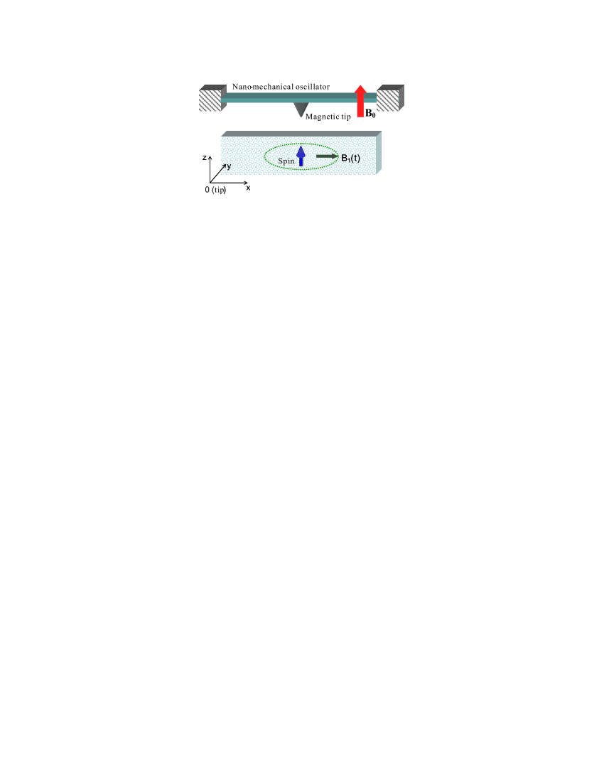
Figure 1: (Color online) The setup of the spin and the nanomechanical resonator. They are coupled with each other by a tiny ferromagnetic particle attached on the NAMR.

The schematics of the coupling system of the spin and the NAMR is illustrated in Fig.1. It is similar to that of the MRFM, but here the NAMR is quantized, since it is assumed to oscillate at GHz under a temperature of mK. A ferromagnetic particle is glued on the middle of the NAMR and exerts a gradient magnetic field on the spin below. Besides, there are also a static magnetic field $B_{0}$ pointing in the $z$-direction and a rotating RF magnetic field $B_{1}(t)$ imposed on the spin.

The magnetic tip produces a dipole magnetic field at the position of the spin Jackson1999 :

$$\vec{B}_{tip}=\frac{\mu_{0}}{4\pi}\frac{3(\vec{n}\cdot\vec{m})\vec{n}-\vec{m}}{r^{3}},$$ (1)

where $\mu_{0}$ is the vacuum magnetic conductance, $\vec{n}$ the unit vector from the tip to the spin, $\vec{m}$ the magnetic moment of the ferromagnetic particle pointing in the $z$-direction, $r$ the distance between the tip and the spin. The reference frame is established with the origin point at the balance position of the magnetic tip. For the sake of the simplicity we assume that the spin is exactly beneath the tip and the NAMR with the magnetic tip oscillates in the $x-z$ plane. The coordinate of the spin is set to be $(0,0,d)$. As the vibration amplitude of the NAMR (the magnetic tip) is very small comparing to the distance between the tip and the spin, the magnetic field at the position of the spin produced by the magnetic tip is approximately written as

$$\vec{B}_{tip}(z)=(A-Gz)\hat{e}_{z}$$ (2)

to the first order of approximation. Here, $z$ is the small deviation of the magnetic tip from its balance position; $\hat{e}_{k}$ ($k\in\{x,y,z\}$) is the unit vector for the $x,y,z$ axis respectively; $A=\mu_{0}m/(2\pi d^{3})$ and $G=3\mu_{0}m/(2\pi d^{4})$.

The NAMR with the magnetic tip is modelled as a harmonic oscillator in the lowest order of approximation, which is quantized in the following. The Hamiltonian of the coupling system reads

$$H=\frac{p_{z}^{2}}{2m_{eff}}+\frac{1}{2}m_{eff}\omega_{c}^{2}z^{2}+\gamma\hbar\vec{B}\cdot\vec{S},$$ (3)

where $m_{eff}$ is the effective mass of the harmonic oscillator, $p_{z}$ the canonical momentum, $\omega_{c}$ its frequency, $-\gamma$ the gyromagnetic ratio and

$$\vec{B}=B_{0}\hat{e}_{z}+\vec{B}_{1}(t)+\vec{B}_{tip}(z).$$ (4)

is the  total magnetic field .The RF magnetic field $\vec{B}_{1}(t)$ is

$$\vec{B}_{1}(t)=B_{1}\cos(\omega_{r}t+\varphi)\hat{e}_{x}+B_{1}\sin(\omega_{r}t+\varphi)\hat{e}_{y}$$ (5)

with $B_{1}$ being its amplitude, $\omega_{r}$ its frequency and $\varphi$ its phase. By performing a “rotating reference frame” transformation in the $x$-$y$ plane, the time dependence of $\vec{B}_{1}(t)$ can be eliminated. Then in the rotating frame rotating around the $z$-direction at the frequency $\omega_{r}$, the effective RF magnetic field reads

$$B_{1}^{\prime}=(\omega_{r}/\gamma)\hat{e}_{z}+B_{1}(\cos\varphi\hat{e}_{x}+\sin\varphi\hat{e}_{y}).$$ (6)

By defining the bosonic operators $a^{\dagger}$ and $a$, the momentum and coordinate operators $p_{z}$ and $z$ can be expressed as their linear combinations:

$$z=\sqrt{\frac{\hbar}{2m_{eff}\omega_{c}}}(a^{\dagger}+a),p_{z}=i\sqrt{\frac{m_{eff}\omega_{c}\hbar}{2}}(a^{\dagger}-a).$$ (7)

In the rotating reference frame the Hamiltonian of the coupling system can be rewritten as $H=H_{B}+H_{S}+H_{I}$, where

$$H_{B}=(a^{\dagger}a+\frac{1}{2})\hbar\omega_{c}$$ (8)

is the Hamiltonian of the NAMR,

$$H_{S}=\gamma\hbar[B_{1}(\cos\varphi\tilde{S}_{x}+\sin\varphi\tilde{S}_{y})+(B_{0}+A+\frac{\omega_{r}}{\gamma})\tilde{S}_{z}]$$ (9)

is the Hamiltonian of the spin part and

$$H_{I}=-\gamma\hbar\lambda G\tilde{S}_{z}(a^{\dagger}+a)$$ (10)

describes the interaction between the spin and the NAMR. Here, $\tilde{S}_{k}=(1/2)\sigma_{k}$ ($k\in\{x,y,z\}$) are the spin operators and $\lambda\equiv\sqrt{{\hbar}/({2m_{eff}\omega_{c}})}$.

We set

$$B_{0}+A+\frac{{\omega_{r}}}{{\gamma}}=0$$ (11)

with the special setup parameters, i.e., the frequency of the RF magnetic field is just at the resonant point. By rotating the axes of spin as: $S_{z}\equiv\tilde{S}_{x}$, $S_{y}\equiv\tilde{S}_{y}$ and $S_{x}\equiv-\tilde{S}_{z}$, we obtain the following Hamiltonian for the coupling system:

$$H = \hbar\omega_{c}(a^{\dagger}a+\frac{1}{2})+\gamma\hbar B_{1}(\cos\varphi S_{z}+\sin\varphi S_{y})$$ (12)

$$+\hbar g(a^{\dagger}S_{-}+aS_{+}+aS_{-}+a^{\dagger}S_{+}),$$

where $a^{\dagger}$ and $a$ are creation and annihilation operators for the NAMR, $S_{\pm}\equiv S_{x}\pm iS_{y}$ are raising and lowering operators for the spin respectively, and the coupling constant between the mechanical oscillator and the spin is $g\equiv\gamma\lambda G/2$. In the following sections we will explore two quantum features of this spin-boson model in two cases: on-resonance and off-resonance situation.

III Dynamically squeezing of the oscillation of the nanomechanical resonator

In the case of off-resonance situation, there is no obvious exchange of energy between the spin and NAMR, but the squeezing effects of the oscillations of the NAMR appear because of the interference of the two oscillation modes with respect to the two eigenstates of the spin. As is well known, the squeezed state is one kind of minimum-uncertainty state. The quantum fluctuation of one quadrature component of the squeezed state is less than that of the coherent state. Thus the uncertainty of the position or the momentum of the squeezed NAMR may be reduced below that in standard quantum limit SQL . In the following we will show that the oscillation of the NAMR can be squeezed by the off-resonance interaction with the spin. Similar quantum squeezing of mechanical motion for the NAMR is discussed by Blencowe and Wybourne with the capacitive coupling NAMR and its substrate Blencowe2000 , and by Wang et al. with the NAMR coupling to a Cooper pair box WYD2004 .

The off-resonance interaction, i.e., in large detuning situation $g\ll\Delta\equiv|\omega_{s}-\omega_{c}|$, Hamiltonian (12) can be approximately written in a diagonal form by adiabatically eliminating coherent effect between the spin states $|0\rangle$ and $|1\rangle$ WYD2004 :

$$H_{diag}=\sum_{k=0,1}H_{k}\otimes|k\rangle\langle k|,$$ (13)

where we have put $\varphi=0$ in Hamiltonian (12). The explicit form of $H_{k}$ is

$$H_{k} \approx \omega_{c}a^{\dagger}a+\frac{(-1)^{k}}{2}\omega_{s}$$ (14)

$$-\frac{(-1)^{k}g^{2}}{4\Delta}(a^{\dagger}a^{\dagger}+2a^{\dagger}a+aa+1),$$

where $\omega_{s}=\gamma B_{1}$.

To diagonalize each effective Hamiltonian $H_{k}$, we use the Bogliubov transformation or the called squeezing transformation:

$$b_{k}=\mu_{k}a-\nu_{k}a^{\dagger},$$ (15)

where the parameters

$$\mu_{k} = \frac{1}{2}\left(\sqrt{N_{k}}+\frac{1}{\sqrt{N_{k}}}\right),$$

$$\nu_{k} = \frac{1}{2}\left(\sqrt{N_{k}}-\frac{1}{\sqrt{N_{k}}}\right)$$ (16)

are defined in terms of

$$N_{k}=\sqrt{\frac{\omega_{c}\Delta}{\omega_{c}\Delta-(-1)^{k}g^{2}}}.$$ (17)

The diagonal Hamiltonian then reads

$$H_{k}=\Omega_{k}(b_{k}b_{k}^{\dagger}+\frac{1}{2})+E_{k}(-1)^{k}(\frac{\omega_{s}}{2}-\frac{g^{2}}{4\Delta}),$$ (18)

where $E_{k}(0)=(-1)^{k}(\omega_{s}/2-g^{2}/(4\Delta)).$ The eigen-frequency

$$\Omega_{k}\approx\omega_{c}\left(1-(-1)^{k}\frac{g^{2}}{2\omega_{c}\Delta}\right).$$ (19)

contains a term $\delta=g^{2}/2\omega_{c}\Delta,$ which is called AC Stark shift and is essentially due to the Lamb effect.

Since the coherent state of the NAMR is most close to the classical one, it seems to be feasible to prepare the NAMR in this state. Starting from the coherent state $\left|\alpha\right\rangle$, at time $t$ the NAMR will evolve into

$$\left|\Psi\left(t\right)\right\rangle_{k}=e^{-i\Omega_{k}b_{k}^{{\dagger}}b_{k}t}\left|\alpha\right\rangle$$ (20)

with respect to the spin state $|k\rangle$ according to the above discussion.

To evaluate the squeezing property of $\left|\Psi\left(t\right)\right\rangle_{k}$, we first consider $B_{k}\left(t\right)\left|\Psi\left(t\right)\right\rangle_{k}$, where

$$B_{k}\left(t\right)=\mu_{k}(t)b_{k}+\nu_{k}(t)b_{k}^{{\dagger}}$$ (21)

is the time evolution of the Heisenberg operators $b_{k}$, and is found to be dynamical squeezing operators. Here, the time-dependent coefficients are

$$\mu_{k}(t)=\mu_{k}e^{i\Omega_{k}t},\nu_{k}(t)=\nu_{k}e^{-i\Omega_{k}t}.$$ (22)

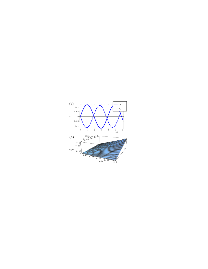
Figure 2: (Color online) (a) The squeezing factor $r_{k}$ of the oscillation of the NAMR initially in the coherent state $|\alpha\rangle$ for the different state $|k\rangle$ of the spin. (b) The maximum squeezing factor $lnN_{k}$. The detuning $g/\Delta\in[0.01,0.1]$ and coupling strength $g/\omega_{c}\in[0.01,0.99]$.

In fact, the state $\left|\Psi\left(t\right)\right\rangle_{k}$ of the NAMR is the eigenstate of squeezing operator $B_{k}\left(t\right)$ and the corresponding eigenvalue is $\alpha$:

$$B_{k}\left(t\right)\left|\Psi\left(t\right)\right\rangle_{k}=\alpha\left|\Psi\left(t\right)\right\rangle_{k}.$$ (23)

Now we can write the quasi-excitations of $B_{k}(t)$ and $B_{k}(t)^{\dagger}$ in terms of the elementary photon mode of $a$ and $a^{\dagger}$:

$$B_{k}\left(t\right)=u_{1}\left(t\right)a+u_{2}\left(t\right)a^{\dagger},$$ (24)

where

$$u_{1}\left(t\right) = \cos\Omega_{k}t+i\left(\mu_{k}^{2}+\nu_{k}^{2}\right)\sin\Omega_{k}t,$$ (25)

$$u_{2}\left(t\right) = 2i\mu_{k}\nu_{k}\sin\Omega_{k}t,$$ (26)

and

$$\left|u_{1}\left(t\right)\right|^{2}-\left|u_{2}\left(t\right)\right|^{2}=1.$$ (27)

According to Eq.(23), the time evolution of the NAMR in the case of off-resonance follows the eigenstate of the quasi-excitation of $B_{k}(t)$. And the eigenstate of $B_{k}\left(t\right)$ is found to be squeezed state with respect to the elementary excitation of the NAMR of $a$ and $a^{\dagger}$. The squeeze factor is calculated as

$$r_{k}\left(t\right)=\ln\left(2\mu_{k}\nu_{k}\sin\Omega_{k}t+\sqrt{1+4\mu_{k}^{2}\nu_{k}^{2}\sin^{2}\Omega_{k}t}\right).$$ (28)

The dynamical squeezings of the oscillations of the NAMR are plotted in Fig.2 (a), in which the time is in the unit of $1/g$. Depending on the spin state $|k\rangle$, the NAMR is dynamically squeezed with different frequencies $\Omega_{k}$ and with also the different maximum squeeze factor $\ln N_{k}$. The maximum squeezing $\ln N_{k}$ of the oscillation of the NAMR depends on the detuning $g/\Delta$ and the strength of coupling $g/min\{\omega_{c},\omega_{s}\}$, which is shown in Fig.2 (b). Here, we have assumed that $\omega_{c}<\omega_{s}$ in the plotting for convenience. The greater squeezing occurs with smaller detuning and stronger coupling. To guarantee the large detuning assumption in the above discussions, the detuning can not be too small. However, large squeezing can still be attained with the appropriate coupling strength.

Similar to the JC model, in large detuning situation this spin-boson system exhibits “collapse-revival” phenomenon. When the NAMR is initially prepared in the coherent state $\left|\alpha\right\rangle$, its position $\langle x\rangle_{t}$ can be calculated by noticing the fact that the time evolution of the NAMR always follows the eigenstate of quasi-excitation $B_{k}\left(t\right)$. Therefore, we expand $a+a^{{\dagger}}$ in terms of $B_{k}\left(t\right)$ and $B_{k}^{{\dagger}}\left(t\right)$, then $\left\langle x\right\rangle_{t}=\left\langle a+a^{{\dagger}}\right\rangle_{t}$ is calculated as

$$\left\langle x\right\rangle_{t} = \sum_{k}c_{k}c_{k}^{\ast}(\alpha\left[\frac{1}{N_{k}}\cos\Omega_{k}t-i\sin\Omega_{k}t\right]$$ (29)

$$+\alpha^{\ast}\left[\frac{1}{N_{k}}\cos\Omega_{k}t+i\sin\Omega_{k}t\right]),$$

where the spin is prepared in the state $c_{0}|0\rangle+c_{1}|1\rangle$ initially. When the spin is prepared in the superposition states, the oscillation of the NAMR collapses and revives, as illustrated in Fig.3. This is the result of the interference effect of the two oscillating mode $\Omega_{k}$ labelled by the spin state $|k\rangle$, which is a witness of the quantization of the NAMR.

Figure 3: Oscillating of the NAMR under off-resonance situation for the system of the NAMR and the spin.

IV Switching between JC Hamiltonian and anti-JC Hamiltonian

When the spin resonate with the NAMR, under the rotating wave approximation, one can obtain the JC model or anti-JC model from the spin-boson model of Eq.(12). Then the spin and the NAMR form a “mechanical QED” structure – an analog of the cavity QED. It is exciting that the “mechanical QED” offers a new analogue of cavity QED among various solid state cavity QED systems Armour2002 ; Irish2003 ; Blais2004 ; Wallraff2004 ; Chiorescu2004 ; Wang2004 .

Without loss of generality, in the following we assume that $B_{1}>0$. When the phase of the RF magnetic field $\varphi=0$, the Hamiltonian (12) becomes a JC Hamiltonian

$$H_{JC} = \hbar\omega_{c}(a^{\dagger}a+\frac{1}{2})+\hbar\omega_{s}S_{z}+\hbar g(a^{\dagger}S_{-}+aS_{+}),$$

under the rotating wave approximation. Here $\omega_{s}=\gamma B_{1}>0$. This can be understood in the interaction picture, in which the term

$$F_{1}=e^{-i(\omega_{c}+\omega_{s})t/\hbar}aS_{-}+e^{i(\omega_{c}+\omega_{s})t/\hbar}a^{\dagger}S_{+}$$ (31)

oscillates fast with higher frequency, and thus can be neglected. For this JC Hamiltonian in the large detuning limit $g/\Delta\ll 1$, where $\Delta=|\omega_{c}-\omega_{s}|$, the dressed energy level of the NAMR is $\omega_{c}+{2g^{2}}\langle S\rangle/{\Delta}$.

When the phase of the RF magnetic field $\varphi=\pi$, the Hamiltonian (12) becomes an anti-JC Hamiltonian

$$H_{AJC}=\hbar\omega_{c}(a^{\dagger}a+\frac{1}{2})+\hbar\omega_{s}S_{z}+\hbar g(aS_{-}+a^{\dagger}S_{+}),$$

(32)

under the rotating wave approximation. Here $\omega_{s}=-\gamma B_{1}<0$. This can be understood in the interaction picture, in which the term

$$F_{2}=e^{-i(\omega_{c}-\omega_{s})t/\hbar}aS_{+}+e^{i(\omega_{c}-\omega_{s})t/\hbar}a^{\dagger}S_{-},$$ (33)

rather than $F_{1}$, oscillates fast with higher frequency, thus should be neglected. For this anti-JC Hamiltonian at the large detuning situation, the dressed energy level of the NAMR reads $\omega_{c}-{2g^{2}}\langle S\rangle/{\Delta}$.

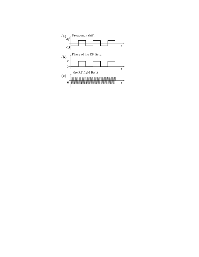
Figure 4: Timing diagram for switching the coupling system between the JC and the anti-JC Hamiltonian. The initial state of the spin is supposed to be the ground state of the JC Hamiltonian. The frequency shift $\delta f={g^{2}}/{\Delta}$ of the NAMR changes its sign when the system switches between the two Hamiltonians, while the state of the spin evolves little.

In the two situations of the JC and the anti-JC models that we discussed above, it is noticed that the AC Stark shifts have opposite signs. This motivates us to present a scheme for the single spin detection. The trick is similar to the interrupted oscillating the cantilever-driven adiabatic reversals (iOSCAR) protocol Rugar2004 , and provide a convenient frequency shift detection without requesting the difficult measurement of the absolute frequency of the NAMR. The RF magnetic field is interrupted for half a cycle periodically as illustrated in Fig.4 (c). Then the phase of the RF magnetic field $\varphi$ will swing between $0$ and $\pi$ correspondingly, which is illustrated in Fig.4 (b). Therefore, as discussed above, the “mechanical QED” of the NAMR and the spin switches between the JC Hamiltonian and the anti-JC Hamiltonian. When the switching is fast enough so that the spin only evolves little and is kept in its original state, i.e., the expectation of the spin $\langle S\rangle$ keeps its value, the frequency shift of the NAMR swings between ${2g^{2}}\langle S\rangle/{\Delta}$ and $-{2g^{2}}\langle S\rangle/{\Delta}$ periodically as the consequence of this Hamiltonian switching, which is illustrated in Fig.4 (a).

To discuss the frequency shifts of the NAMR with concrete parameters in practical experiments, we write down the expression of the coupling constant

$$g=\gamma G\sqrt{\frac{\hbar}{8m_{eff}\omega_{c}}}\approx 10^{-7}G\sqrt{\frac{\omega_{c}}{k_{eff}}}$$ (34)

explicitly, here $k_{eff}$ is the effective spring constant of the mechanical oscillator. Substituting the parameters of Ref.Rugar2004 , where $G\sim 10^{5}$ T/m, $k_{eff}=0.11$ mN/m and $\omega_{c}=5.5$ kHz, in the above equation, we obtain a frequency shift about 7 Hz for the NAMR. Here we have supposed the detuning $g/\Delta=0.1$. The frequency shift is larger than that in the current OSCAR technique (about 4 mHz in Ref.Rugar2004 ) by three orders of magnitude. In the OSCAR the NAMR is treated as a classical oscillator. Therefore, if the temperature of the system can be reduced to $\hbar\omega_{c}/k_{B}=42$ nK so that it enters the quantum regime, mechanical QED model indeed provides an efficient protocol for single electron spin detection.

There are some protocols Hopkins2003 ; Hohberger2004 ; Zhang2005 that promise to cool the temperature of the NAMR down to mK or even lower. However reducing the temperature of the NAMR still remains a great challenge in the experiments. To our best knowledge, the lowest temperature attained in the dilution fridge now is about 30 mK. So we consider another way to push the NAMR into the quantum regime by increasing its frequency rather than decreasing its temperature. Unfortunately, the effective spring constant of the simple structure resonator increases rapidly with the oscillator frequency: $k_{eff}\propto\omega_{c}^{2}$. When the frequency of the NAMR increases, the coupling constant $g\propto 1/\sqrt{\omega_{c}}$ decreases. Therefore a much smaller frequency shift about 0.01 Hz occurs for a 1.5 GHz nanomechanical oscillator with the simple structure like the one in Ref.Rugar2004 , which makes it hard to be detected in the experiments. However, in Ref.Gaidarzhy2005 , an elaborately designed nanomechanical resonator with an antenna structure reaches the frequency of 1.5 GHz with a smaller effective spring constant about 300 N/m. Therefore, for this enhanced resonator, the frequency shift is about 3 Hz , which is larger than that of the simple structure resonator by about two orders of magnitude. As indicated in Eq.(34) stronger coupling constant $g$ can be reached by increasing the magnetic field gradient and decreasing the effective spring constant of the nanomechanical resonator. The stronger the coupling is, the larger frequency shifts is obtained.

Developments in the experiments are still necessary to practise the presented protocol in detecting single spin. However, as no adiabatic condition is requested in this protocol, the frequency of the NAMR can be set to resonant with the spin, while for the single spin detection with the OSCAR technique, such as Ref.Rugar2004 ; Berman2005 , the frequency of the NAMR must be much smaller than that of the spin. So if one sets the frequency of the NAMR at MHz, then a micro Kelvin temperature is sufficient to prepare the NAMR in the ground state, which is much more realizable in the experiments in the near future. And the frequency shift to be detected is about tens Hz. The required resolving power is about $10^{-6}$. It is the same to that of the OSCAR MRFM mHz/kHz= $10^{-6}$ Rugar2004 , which has already been achieved in the experiments. There is indeed no fundamental difficulty of the above suggested single spin detection. Actually there are still space to further optimize the frequency of the NAMR to balance the resolving power and the temperature to be attained. The discussion in this section suggests a single spin detection in the absence of the environment, which is far from the reality. In the next section we will discuss the influence of the thermal environments on the NAMR.

V Damping of the nanomechanical resonator

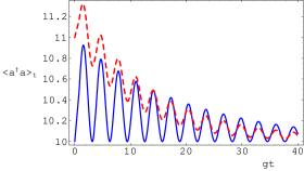
Figure 5: (Color on line) The damping of the NAMR. The energy of the NAMR $\langle a^{\dagger}a\rangle_{t}$ is plotted with the NAMR or spin in excited state under weak coupling environment situation $\kappa/g=0.2$. The red(dashing) line is for the NAMR initially in the excited state, and the blue(solid) line is for the spin initially in the excited state.

In the above discussions, we demonstrate various quantum optical phenomena due to the quantization of the NAMR. But due to the coupling to the complex environments in practice, these phenomena may be washed out. Therefore it is necessary to study the influence of environments. Both the spin and the NAMR are coupled to the environments, which causes the system damp their energy into the environments in thermal equilibrium. It is suggested by the experiments of the MRFM that the spin has longer relaxation time than the NMR Rugar2004 . For the detailed discussions about the dissipation in the NAMR, one can refer to Ref. Mohanty2002 ; Berman2003 ; Gassmann2004 . The damping behavior of the total system is mainly dominated by that of the NAMR. In general, we model the environment as a multi-mode boson bath coupling to the NAMR. The total Hamiltonian of the coupling system of the NAMR and the spin and the environment reads

$$H_{total}=H+\sum_{j}\hbar\omega_{j}b_{j}^{\dagger}b_{j}+\hbar\sum_{j}k_{j}(a^{\dagger}b_{j}+ab_{j}^{\dagger}).$$ (35)

Here , $\ H$ is the Hamiltonian (12) of the total system, $b_{j}$ and $b_{j}^{\dagger}$ are creation and annihilation operators of the $j$th mode of the environment, $k_{j}$ is the coupling constant between the NAMR and the $j$th mode of the environment. We neglect various two-excitation processes, and terms such as $ab_{j}$ and $a^{\dagger}b_{j}^{\dagger}$ are omitted in the total Hamiltonian.

We invoke Heisenberg-Langevin method to deal with this quantum damping problem. The operators $(a^{\dagger})^{m}a^{n}O$, ($O=S_{z},S_{\pm}$), satisfy the following equations: Scully

$$\frac{d}{dt}[(a^{\dagger})^{m}a^{n}O]=-\frac{i}{\hbar}[(a^{\dagger})^{m}a^{n}O,H]$$

$$+(i\kappa Q(m-n)-\frac{1}{2}\kappa(m+n))\langle(a^{\dagger})^{m}a^{n}\rangle_{E}$$

$$+\kappa mnn_{th}\langle(a^{\dagger})^{m-1}a^{n-1}\rangle_{E},$$ (36)

where $\kappa$ is the damping factor, $Q$ the quality factor of the NAMR, and $\langle...\rangle_{E}$ represents tracing of the environment.

The higher order processes, such as the terms $ab_{j}$ and $a^{\dagger}b_{j}^{\dagger}$, of the NAMR are neglected in the following discussions. Therefore the expectations of the operators including quadratic or higher powers in operators $a$ and $a^{\dagger}$ of the NAMR, such as $\langle a^{2}\rangle$ and $\langle a^{\dagger 2}S_{z}a\rangle$, are zero. With these approximations we simultaneously obtain the closed system of equations:

$$\frac{d\langle a^{\dagger}a\rangle}{dt} = -\kappa\langle a^{\dagger}a\rangle+gX+\kappa n_{th}$$ (37)

$$\frac{d\langle S_{z}\rangle}{dt} = -2gX$$ (38)

$$\frac{dX}{dt} = g\langle S_{z}\rangle-\frac{1}{2}\kappa X+2g\langle a^{\dagger}S_{z}a\rangle+g$$ (39)

$$\frac{d\langle a^{\dagger}S_{z}a\rangle}{dt} = -gX-\kappa\langle a^{\dagger}S_{z}a\rangle$$ (40)

where $n_{th}$ is the average thermal photons in the environment, and $X=i\langle S^{+}a+S^{-}a^{\dagger}\rangle$. The above system of equations can be solved by Laplace transform method or numerically. In Fig.5 under situation of weak coupling to the environment, we plot the time evolving of the expectation of the energy of the NAMR $\langle a^{\dagger}a\rangle$ with the initial condition $n_{th}=10$, $\langle a^{\dagger}a\rangle+\langle S_{z}\rangle=11$, $X=\langle a^{\dagger}S_{z}a\rangle=0$. The case of stronger coupling to the environment, i.e., larger $\kappa/g$, is also studied. It is not surprising that the oscillation of the energy of the NAMR die out faster with larger $\kappa/g$, and with sufficient strong coupling to environment, no oscillation of the energy of the NAMR could be observed. This simple consideration suggests that even for non-zero temperature it is still possible to observe the energy oscillation between the NAMR and the spin as long as the coupling to the environment is weak enough.

VI Summary and Remarks

We have revisited a spin-boson model for the coupling system of the nanomechanical resonator and the spin. With the same blocks (the NAMR with a mgnetic tip and the spin) as that in the MRFM, but with the refined setup parameters, the NAMR enters the quantum regime and thus a fully quantum theory is needed. With the quasi-classical state (the coherent state) as the initial state of the NAMR, the dynamical squeezing of the mode and also the oscillation of the NAMR is studied under the large detuning limit. Both the coherent state and the low frequency (large detuning) of the macro-size resonator are preferred in the experiments. Squeezed states, even if there is the thermal noise and the displacement, can have non-classical properties, such as bunch distribution of phonon numberMarian1993a ; Marian1993b ; Lu2000 . With the model setup and the predications of the quantum optical phenomena, we actually describe a cavity QED analog for the quantum dynamics of the coupling system. For the quantized NAMR, the spin-boson model for this coupling system can refer to a JC or an anti-JC model according to different physical accessible parameters. By modulating the phase of RF magnetic field one can switch the system between the JC and anti-JC model. This observation provides a potential protocol for the detection of the single spin.

Acknowledgments: This work is supported by the NSFC with grant Nos. 90203018, 10474104, 60433050 and 10574133. It is also funded by the National Fundamental Research Program of China with Nos. 2001CB309310 and 2005CB724508. We also thank Y.D. Wang and Yong Li for helpful discussions.

References

- (1) X.M.H. Huang, C.A. Zorman, M. Mehregany and ML Roukes, Nature (London) 421, p496 (2003).
- (2) A. N. Cleland and M. R. Geller, Phys. Rev. Lett. 93, 070501, (2004).
- (3) A. Gaidarzhy, G. Zolfagharkhani, R. L. Badzey and P. Mohanty, Phys. Rev. Lett. 94, 030402 (2005).
- (4) A. Gaidarzhy, G. Zolfagharkhani, R. L. Badzey and P. Mohanty, Appl. Phys. Lett. 86, 254103 (2005).
- (5) Igor Bargatin and M. L. Roukes, Phys. Rev. Lett. 91 138302 (2003).
- (6) C. P. Sun, L. F. Wei, Yu-xi Liu, and Franco Nori, Phys. Rev. A 73, 022318 (2006).
- (7) D. Rugar, R. Budakian, H. J. Mamin and B. W. Chui, Nature 430, p329 (2004).
- (8) G. P. Berman, F. Borgonovi, V.N.Gorshkov and V. I. Tsifrinovich, IEEE Transactions on Nanotechnology 4, p14-20 (2005).
- (9) John David Jackson, 1999, 3rd Ed., Classical Electrodynamics, p186, (John Willey & Sons Inc. Press).
- (10) V. B. Braginsky, F.Y. Khalili, Quantum Measurement, Cambridge Univ Pr (June 1995).
- (11) M. P. Blencowe and M. N. Mybourne, Physica B(LT 22 Proceedings) 280, p555, (2000).
- (12) Y. D. Wang, Y.B. Gao and C. P. Sun, Eur. Phys. J. B 40, p321-326, (2004).
- (13) A. D. Armour, M. P. Blencowe and K. C. Schwab, Phys. Rev. Lett. 88, 148301 (2002).
- (14) E. K. Irish and K. Schwab, Phys. Rev. B 68, 155311 (2003)
- (15) A. Blais, R. Huang, A. Wallraff, S. Girvin and R. Schoelkopf, Phys. Rev. A 69, 062320 (2004)
- (16) A. Wallraff, D. L. Schuster, A. Blais, L. Frunzio, R. -S. Huang, J. Majer, S. M. Girvin and R. J. Schoelkopf, Natrue 431, p162 (2004).
- (17) I. Chiorescu, P. Bertet1, K. Semba, Y. Nakamura, C. J. P. M. Harmans and J. E. Mooij, Nature 431, p159 (2004).
- (18) Y. D. Wang, P. Zhang, D. L. Zhou, and C. P. Sun, Phys. Rev. B 70, 224515 (2004).
- (19) Asa Hopkins, Kurt Jacobs, Salman Habib and Keith Schwab, Phys. Rev. B 68, 235328 (2003).
- (20) Constanze Höhberger Metzger and Khaled Karral, Nature 432, p1002 (2004).
- (21) P. Zhang, Y. D. Wang, and C. P. Sun, Phys. Rev. Lett. 95, 097204 (2005).
- (22) P. Mohanty, D. A. Harrington, K. L. Ekinci, Y. T. Yang, M. J. Murphy and M. L. Roukes, Phys. Rev. B 66, 085416 (2002).
- (23) G. P. Berman, F. Borgonovi, Hsi-Sheng Goan, S. A. Gurvitz, and V. I. Tsifrinovich, Phys. Rev. B 67, 094425 (2003).
- (24) Hanno Gassmann, Mahn-Soo Choi, Hangmo Yi, and C. Bruder, PRB 69, 115419 (2004).
- (25) M.O. Scully, M.S Zubairy, Quantum Optics, Cambridge University Press (January 1997)
- (26) Paulina Marian and Tudor A. Marian, Phys. Rev. A 47, 4474 (1993)
- (27) Paulina Marian and Tudor A. Marian, Phys. Rev. A 47, 4487 (1993)
- (28) W-F. Lu, J. Phys. A: Math. Gen. 33 479 (2000).