Single photon continuous variable quantum key distribution based on energy-time uncertainty relation

Abstract

In previous quantum key distribution (QKD) protocols, information is encoded on either the discrete-variable of single-photon signal or continuous-variables of multi-photon signal. Here, we propose a new QKD protocol by encoding information on continuous-variables of a single photon. In this protocol, Alice randomly encodes her information on either the central frequency of a narrowband single photon pulse or the time-delay of a broadband single photon pulse, while Bob randomly chooses to do either frequency measurement or time measurement. The security of this protocol rests on the energy-time uncertainty relation, which prevents Eve from simultaneously determining both frequency and time information with arbitrarily high resolution. In practice, this scheme may be more robust against various channel noises, such as polarization and phase fluctuations.

Unlike conventional cryptography, quantum key distribution (QKD) provides unconditional security guaranteed by the fundamental laws of quantum physics BB84 ; A91 ; Gisin02 ; securityproof . To date, both discrete-variable, single-photon QKD protocols (such as the well-known BB84 protocol BB84 )and continuous-variable, multi-photon QKD protocols (such as QKD with squeezed statesSqueeze ) have been developed. In the standard BB84 protocol BB84 ; BB84more , one of the legitimate users, Alice, encodes information in a two-dimensional subspace (such as the polarization state) of a single photon. The security is based on the no-cloning theorem nonclone . In contrast, in a continuous variable QKD (CV-QKD), information is encoded on field quadratures of either squeezed states or coherent statesSqueeze ; CV (We name this scheme as quadrature-coding CV-QKD to distinguish it from the new protocol we will present). Quantum mechanically, the complex field amplitudes correspond to a pair of non-commuting operators $X_{1}$ and $X_{2}$. The security of this protocol follows from the uncertainty relation for these two operators Squeeze

$$\Delta X_{1}\Delta X_{2}\geq 1/4,$$ (1)

It is thus impossible to measure both of them arbitrarily accurately.

However, there are a few practical difficulties in telecom fiber-based QKD. In both the phase-coding BB84 QKD system and the quadrature-coding CV-QKD system, the quantum bit error rate (QBER) is closely related to the interference visibility, which suffers from polarization and phase instabilities induced by the optical fiber. A Bidirectional auto-compensating structure has been introduced to improve the performance of a practical QKD systemPP . Unfortunately, this design also opens a potential back-door for the eavesdropper (Eve) to launch various Trojan horse attacks trojan .

Normally, the frequency of a weak laser pulse won’t change as it propagates through fiber, and the temporal broadening can be well controlled by employing dispersion-compensation techniques. This inspires us to explore a frequency/time coding QKD protocol.

We remark that QKD protocols based on frequency-coding have been studied previouslyprevious1 ; previous2 ; previous3 . In previous workprevious2 : Alice represents bit 0 and bit 1 with two distinguishable signal states $S_{0}$ (a single photon state with frequency $\omega_{0}$) and $S_{1}$ (frequency $\omega_{1}$). She randomly prepares either one of the two signal states or a control state $S_{c}$, which is a superposition of $S_{0}$ and $S_{1}$. At Bob’s side, he randomly chooses to do one of the following three measurements: $S_{0}$ measurement with a narrowband filter centered at frequency $\omega_{0}$ and a single photon detector (SPD), $S_{1}$ measurement with a $\omega_{1}$ filter and a SPD, or time measurement with a time-resolving SPD (no filter). Alice and Bob uses signal states for key distribution and control state for detecting Eve’s attack. Note in the cases when Alice prepares the control states and Bob does the time measurements, a high visibility interference pattern is expected. Any attack from Eve will unavoidably blur the interference pattern and be caught.

We remark that in the above protocolprevious2 , the density matrix for the control state $\hat{\rho}_{c}$ is different from that for the signal states $\hat{\rho}_{s}$ densitymatrix1 . In principle, Eve can unambiguously distinguish them with a non-zero probabilityattack . We remark that to eliminate this information, Alice can randomly prepare two types of control states, $(|\omega_{0}\rangle+exp[i(\omega_{1}-\omega_{0})t]|\omega_{1}\rangle)$ and $(|\omega_{0}\rangle-exp[i(\omega_{1}-\omega_{0})t]|\omega_{1}\rangle)$,with equal probability. In this case, $\hat{\rho}_{s}=\hat{\rho}_{c}=|\omega_{0}\rangle\langle\omega_{0}|+|\omega_{1}\rangle\langle\omega_{1}|$.

In this letter, we propose a single photon CV-QKD protocol: Alice randomly encodes her information on either the central frequency or the time-delay of a transform limited (TL) single photon pulsesync , while Bob randomly does frequency or time measurement. The security of this protocol can be understood from the well-known energy-time uncertainty relation $\Delta E\Delta t\geq\hbar/4$. For a TL Gaussian pulse, it’s easy to show that TL

$$\sigma_{\omega}\sigma_{t}=1,$$ (2)

where $\sigma_{\omega}$ and $\sigma_{t}$ are the half width ($1/e$) of the intensity spectrum and the temporal profile respectively. Eq.(2) indicates that it’s impossible to acquire both the frequency and the time information of a single photon pulse with an arbitrarily high resolution.

Compareing (1) with (2), we can see a high similarity between our protocol and the squeezed states CV-QKD. We remark that the energy-time uncertainty relation may be different fundamentally from others, such as the position-momentum uncertainty relation, because time is not an observable in non-relativistic quantum mechanics. However, this fundamental question is outside the scope of our current paper.

Fig.1 shows a diagram of our proposed QKD system. In Fig.1, Alice randomly fires one of two single photon sources: $S_{1}$ produces narrowband frequency tunable TL Gaussian pulses (bandwidth $\sigma_{\omega 1}$), while $S_{2}$ produces broadband time-delay tunable TL Gaussian pulses(bandwidth $\sigma_{\omega 2}$, central frequency $\omega_{0}$), with $\sigma_{\omega 1}<<\sigma_{\omega 2}$. The frequency tunable range of $S_{1}$ matches the spectrum of $S_{2}$, while the time-delay tunable range of $S_{2}$ matches with the temporal profile of $S_{1}$, as shown in Fig.2. A beam splitter $BS$ is employed to combine the outputs from $S_{1}$ and $S_{2}$ together. At Bob’s side, passively determined by a beam splitter, he can either conduct time measurement with a high-speed time-resolving single photon detector (TSPD), or frequency measurement with a dispersive element (such as a dispersive grating) followed by a single photon detector array (SPDA).

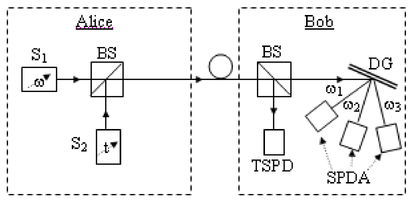
Figure 1: Schematic diagram of the proposed QKD system: $S_{1}$-narrowband frequency tunable single photon source; $S_{2}$-broadband single photon source with tunable time-delay; BS-beam splitter; DG-dispersive grating; TSPD-time-resolving single photon detector; SPDA-single photon detector array.

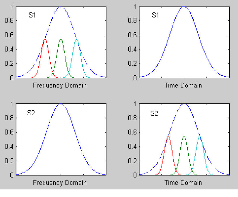
Figure 2: Illustration of the frequency (time) domain distributions of Alice’s single photon sources: top left-$S_{1}$ in frequency domain (note the envelope matches with the spectrum of $S_{2}$); top right-$S_{1}$ in time domain; bottom left-$S_{2}$ in frequency domain; bottom right-$S_{2}$ in time domain(note the envelope matches with the temporal profile of $S_{1}$).

Our QKD protocol runs as follows:

1.Alice generates a binary random number $a$. If $a=0$, she generates another random number $b$ from the Gaussian distribution $f_{1}(b)=(\pi\sigma_{\omega 2}^{2})^{-1/2}exp[-(b-\omega_{0})^{2}/{\sigma_{\omega 2}^{2}}]$; then she sets the central frequency of $S_{1}$ to $b$ and fires it. If $a=1$, Alice generates a random number $b$ from the Gaussian distribution $f_{2}(b)=(\pi)^{-1/2}\sigma_{\omega 1}exp[-{\sigma_{\omega 1}^{2}b^{2}}]$; then she sets the time-delay of $S_{2}$ to $b$ and fires it.

2.Passively determined by a beam splitter, Bob either conducts time measurement with a high-speed time-resolving single photon detector (TSPD), or frequency measurement with a dispersive grating (DG) followed by a single photon detector array (SPDA).

3.They repeat step 1 and step 2 many times.

4.Through an authenticated classical communication channel, they post-select the cases when the quantum states prepared by Alice match with the measurements conducted by Bob. After this step, Alice and Bob share a set of correlated Gaussian variables, which are called ”key elements”.

5.Alice and Bob can use the ”sliced reconciliation” protocol reconciliation to transform the ”key elements” into errorless bit strings.

6.Alice and Bob can estimate the maximum information acquired by Eve from the measured error rate and may use standard privacy amplification protocol to distill out the final secure key.

The security of this protocol is based on: first, Eve can not distinguish frequency-coding photons from time-coding photons; secondly, Eve’s ability to simultaneously determine both the frequency information and the time information is constrained by the uncertainty relation (2). It can be shown that in the asymptotic case when $\sigma_{\omega 1}\rightarrow 0$, the density matrixes of frequency-coding photons and time-coding photons are identicaldensitymatrix2 :

$$\hat{\rho}_{1}=\hat{\rho}_{2}=\int{(\pi\sigma_{\omega 2}^{2})^{-1/2}exp[-(\omega_{1}-\omega_{0})^{2}/{\sigma_{\omega 2}^{2}}]}$$ (3)

$$\times{\hat{a}^{+}(\omega_{1}){|0\rangle\langle 0|}\hat{a}(\omega_{1}){d\omega_{1}}},$$

Here, $\hat{a}^{+}(\omega)$ is the continuous-mode creation operator. In practice, as long as $\sigma_{\omega 1}<<\sigma_{\omega 2}$, the difference between the two density matrixes is negligible.

To demonstrate the feasibility of this protocol, let’s discuss the basic requirements to the system’s parameters. At Alice’s side, the spectral width of $S_{1}$ is $\sigma_{\omega 1}$ with a continuous tunable range of $\sigma_{\omega 2}$, and the pulse width of $S_{2}$ is $\sigma_{t2}=1/\sigma_{\omega 2}$ with a continuous time-delay tunable range of $\sigma_{t1}=1/\sigma_{\omega 1}$. At Bob’s side, the spectral and time resolutions of his measurement device are $\delta_{\omega}$ and $\delta_{t}$ respectively. Further more, Alice and Bob agree to slice each ”key element” into bins of size $\Delta_{t}$ for a time-coding signal or $\Delta_{\omega}$ for a frequency-coding signal. Here, we assume that $\sigma_{\omega 2}\gg\Delta_{\omega}\gg\delta_{\omega}\gg\sigma_{\omega 1}$ and $\sigma_{t1}\gg\Delta_{t}\gg\delta_{t}\gg\sigma_{t2}$ as shown in Fig.3a (for the case of time-coding).

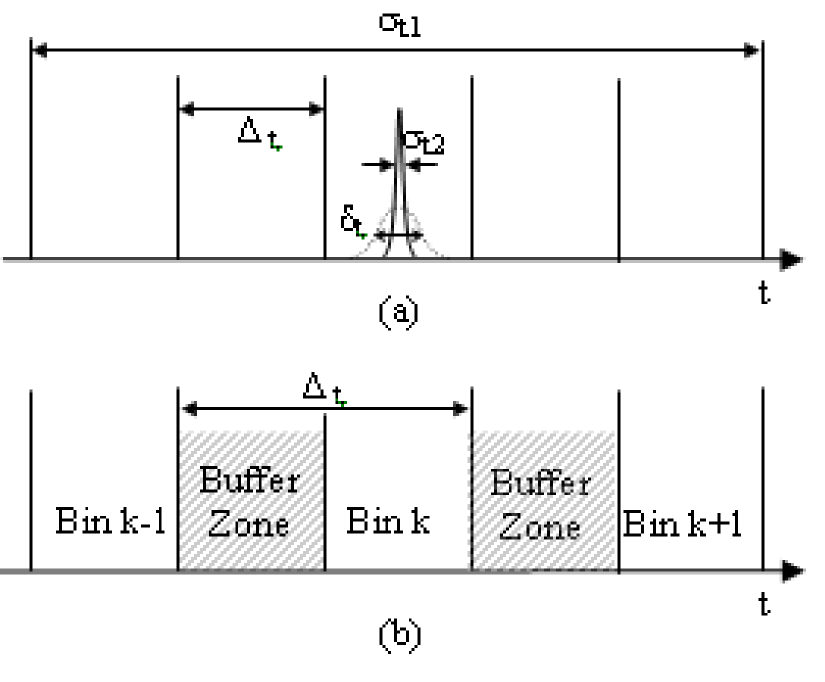
Figure 3: (a) Slice method without ”buffer zone” (for time-coding signal) (b) Slice method with ”buffer zone” between neighbored bins (for time-coding signal)

The error probability of time-coding signals can be estimated as follows: Alice sends out photons at time $t_{c}\in[-\Delta_{t}/2,\Delta_{t}/2]$, with a uniform distribution (for a specific time bin). The intensity distribution in time domain measured by Bob is

$$I(t)=(\pi\delta_{t}^{2})^{-1/2}exp[-(t-t_{c})^{2}/{\delta_{t}^{2}}],$$ (4)

The probability that Bob’s measurement results lies in the interval $[-\Delta_{t}/2,\Delta_{t}/2]$ is

$$P_{\Delta t}=(1/{\Delta_{t}})\int_{-{\Delta_{t}}/2}^{{\Delta_{t}}/2}\int_{-{\Delta_{t}}/2}^{{\Delta_{t}}/2}{I(t)dtdt_{c}},$$ (5)

The error probability $P_{e}=(1-P_{\Delta_{t}})$ can be derived as

$$P_{e}=1-(1/{\sqrt{\pi}S_{t}})[-1+\sqrt{\pi}S_{t}erf(S_{t})+exp(-S_{t}^{2})],$$ (6)

Here, $S_{t}=\Delta_{t}/\delta_{t}$, and $erf(x)$ is the error function which is given by

$$erf(x)=1/\sqrt{\pi}\int_{0}^{x}{exp(-t^{2})dt},$$ (7)

In the case of frequency-coding, we can define $S_{\omega}=\Delta_{\omega}/\delta_{\omega}$ and derive a similar formula.

From (6), to get a low error rate, $S_{t}$ ($S_{\omega}$)has to be large enough. This can be achieved by either increasing the ”bin size” $\Delta_{t}$($\Delta_{\omega}$) or improving Bob’s measurement resolution $\delta_{t}$($\delta_{\omega}$). On the other hand, to guaranty the security of this protocol, the bin sizes have to satisfy the condition of $\Delta_{\omega}\Delta_{t}<1$. These conditions set basic requirements for Bob’s measurement resolutions $\delta_{t}$ and $\delta_{\omega}$measurement . For example, from (6), the error probability $P_{e}$ is about $0.056$ at $S_{t}=10$ for time-coding or $S_{\omega}=10$ for frequency-coding. The requirement for Bob’s apparatus will be $\delta_{t}\delta_{\omega}<0.01$.

We remark that Alice/Bob can improve the slice method by adding in a ”buffer zone” between neighboring bins, as shown in Fig.3b (for the case of time-encoding). In this scenario, Alice and Bob slices their Gaussian variables into discrete bins with a ”buffer zone” between neighbored ones. During the classical communication stage, Alice announces which pulses are prepared in the buffer zone, and they just drop these results. In the case when Alice encodes her information in the ”bin zone”, there are three possible outputs from Bob’s measurement: Bob detects a signal in the same bin with probability $P_{r}$; Bob detects a signal in ”buffer Zones” with probability $P_{b}$ (this is an inconclusive result and they just drop it); or Bob detects a signal in other bins with probability $P_{w}=1-P_{r}-P_{b}$. Define $\Delta_{t}$ as the total size of one bin plus one buffer zone, and assume that the bin size is equal to buffer zone size, then $P_{r}$, $P_{b}$ can be derived as

$$P_{r}=({\Delta_{t}}/2)^{-1}\int_{-{\Delta_{t}}/4}^{{\Delta_{t}}/4}\int_{-{\Delta_{t}}/4}^{{\Delta_{t}}/4}{I(t)dtdt_{c}},$$ (8)

$$P_{b}=({\Delta_{t}}/2)^{-1}\int_{-{\Delta_{t}}/4}^{{\Delta_{t}}/4}\int_{-3{\Delta_{t}}/4}^{3{\Delta_{t}}/4}{I(t)dtdt_{c}}-P_{r},$$ (9)

The error probability is defined as

$$P_{e}=P_{w}/(P_{r}+P_{w}),$$ (10)

For $S_{t}=3$, the error probability $P_{e}$ calculated from (10) is about $0.0038$ while the probability of getting an inconclusive results is about $0.36$. Compared with the slice method without a ”buffer-zone”, the error probability drops by about one order, while the efficiency also drops by a factor of $0.5\times 0.64=0.32$( the $0.5$ factor is because that half of the time Alice sends out signals in the buffer zone, and the $0.64$ factor is due to the inconclusive probability in Bob’s measurement). The requirement for Bob’s apparatus is $\delta_{t}\delta_{\omega}<0.1$, which can be satisfied with today’s technologyresolution . In practice, the buffer size could be optimized to achieve the maximum secure key rate.

The QKD protocol proposed here has several advantages: First of all, a QKD system based on freqnency/time coding is intrinsically insensitive to the polarization and phase fluctuations. This could improve the stability of a fiber-based one-way QKD system dramatically. Secondly, unlike the squeezed states QKD, our protocol can be implemented with commercial laser sources. TL laser pulses with different bandwidths can be easily prepared with commercial products and they can go through long fibers with negligible distortions (For example, in dispersion , after going through a $50km$ fiber, a $460fs$ pulse was slightly broaden to $470fs$. This is orders lower than the time resolution of today’s SPD).Thirdly, compared with previous frequency-coding protocolprevious2 , our system could achieve a higher key rate by using a large alphabet.

We remark that instead of using single photon sources (reliable perfect single photon sources are far from practical), highly attenuated laser sources could be employed to implement our protocol. In this case, to guard against the PNS (photon number splitting) attack, the newly developed decoy state idea can be adopteddecoy .

In conclusion, we propose a new QKD protocol by encoding information on continuous-variables of single photon signals. The security of this protocol rests on the energy-time uncertainty relation, which prevents Eve from simultaneously determine both frequency and time information with arbitrarily high resolution. It will be interesting to see whether a QKD protocol based on the energy-time uncertainty relation is equivalent to the one based on uncertainty relation for two non-commuting operators (such as the squeezed states QKD). In practice, this scheme may be more robust against various channel noises, such as polarization and phase fluctuations.

The author is very grateful to Hoi-Kwong Lo for his supports and helpful comments. The author also thanks Xiong-Feng Ma, Yi Zhao, Ben Fortescue and Chi-Hang Fred Fung for helpful discussions.

References

- (1) C. H. Bennett, G.Brassard, Proceedings of IEEE International Conference on Computers, Systems, and Signal Processing, (IEEE, 1984), pp. 175-179.
- (2) A. K. Ekert, Phys. Rev. Lett. 67 661 (1991)
- (3) N. Gisin, G. Ribordy, W. Tittel, H. Zbinden, Rev. Mod. Phys. 74 145 (2002)
- (4) D. Mayers, J. of ACM 48, 351 (2001); H.-K. Lo, H. F. Chau, Science, 283, 2050 (1999); E. Biham et al. Proceedings of the Thirty-Second Annual ACM Symposium on Theory of Computing (STOC’00) (ACM Press, New York, 2000), pp. 715-724; P. W. Shor, J. Preskill, Phys. Rev. Lett. 85, 441, (2000)
- (5) M. Hillery, Phys. Rev. A 61 022309 (2000)
- (6) R. J. Hughes, J. E. Nordholt, D. Derkacs, C. G. Peterson,New J. Phys. 4 43 (2002); C. Marand, P. D. Townsend, Opt. Lett. 20 1695 (1995); R. J. Hughes, G. L. Morgan, C. G. Peterson, J. Mod. Opt. 47 533 (2000); C. Gobby, Z. L. Yuan, A. J. Shields, Appl. Phys. Lett. 84 3762 (2004)
- (7) W. K. Wootters, W. H. Zurek, Nature 299 802 (2000); D. Dieks, Phys. Lett. A 92 271 (1982)
- (8) T. C. Ralph, Phys. Rev. A 61 010303R (1999); F. Grosshans, G. V. Assche, J. Wenger, R. Brouri, N. J. Cerf, P. Grangier, Nature 421 238 (2003); J. Lodewyck, T. Debuisschert, R. Tualle-Brouri, P. Grangier, Phys. Rev. A 72 050303R (2005)
- (9) A. Muller, T. Herzog, B. Huttner, W. Tittel, H. Zbinden, N. Gisin, Appl. Phys. Lett., 70 793 (1997); M. Legre, H. Zbinden, N. Gisin, arXiv.org:quant-ph/0511113
- (10) N. Gisin, S. Fasel, B. Kraus, H. Zbinden, G. Ribordy, Phys. Rev. A 73 022320 (2006)
- (11) S. N. Molotkov, S. S. Nazin, JETP Lett., 63 924 (1996)
- (12) S. N. Molotkov, JETP, 87 288 (1998)
- (13) B.-S. Shi, Y.-K. Jiang, G.-C. Guo, Appl. Phys. B, 70, 415 (2000)
- (14) The density matrix of the signal states is . The control state can be descried by with a density matrix . In general, .
- (15) Eve could employ a high speed switch which is opened at (when the amplitude of control state is expected to be zero) for a time-duration of . The signal states can pass through this switch with a much higher probability than the control state.
- (16) In practice, for time-coding, the information can be encoded on the time interval between the signal pulse and a synchronization pulse.
- (17) T. D. Donnelly, C. Grossman, Am. J. Phys., 66, 677 (1998).
- (18) G. V. Assche, J. Cardinal, N. J. Cerf, IEEE Trans. Info. Theory, 50, 394 (2004).
- (19) The continuous-mode photon wave-packet creation operator can be defined as . Here, is the spectral amplitude. For a Gaussian pulse with a central frequency of , , where is the time when the peak of the pulse passes the coordinate origin. For , and the central frequency is chosen from . So,the density matrix is . Similarly, we can derive the density matrix for is In the asymptotic case when , We have .
- (20) In practice, the resolutions of Alice’s devices for state preparetion are much higher than the resolutions of Bob’s measurement devices.
- (21) Today’s SPD has a time resolution in the order of , while the spectral resolution of a F-P interferometer can be . This give us .
- (22) Z. Jiang, S.-D. Yang, D. E. Leaird, and A. M. Weiner, Opt. Lett., 30, 1449 (2005).
- (23) W.-Y. Hwang, Phys. Rev. Lett. 91, 057901 (2003); H.-K. Lo, in Proceedings of IEEE ISIT 2004, p. 137; H.-K. Lo, X. Ma, K. Chen, Phys. Rev. Lett. 94 230504 (2005); X. -B. Wang, Phys. Rev. Lett. 94 230503 (2005); X. -B. Wang, Phys. Rev. A 72 012322 (2005); X. Ma et al. Phys. Rev. A 72 012326 (2005); Y.Zhao et al. accepted for publication in PRL, Preprint quant-ph/0503192