An Introduction to Error-Correcting Codes: From Classical to Quantum

Abstract

This report surveys quantum error-correcting codes. As Preskill claimed in Preskill1998-ReliableQC , 21st century would be the golden age of quantum error correction. Quantum channels behave differently from classical channels, so researchers face difficulties in developing robust quantum codes. Fortunately, the classical error control methods have been well developed. If we can learn many lessons from classical coding theory, we can expedite the development of quantum codes. Scientists have discovered that quantum error correction shares many concepts with classical counterpart. Both quantum and classical coding schemes add redundancy to information to protect against noises. They also have similar conditions for error detectability and correctability.

I Introduction

In the age of information technology, error-correcting codes are widely used in communication systems and data storage systems. Both types of systems share the same model, as shown in Fig 1. A source transmits information to a user through a channel. The communication channel, unfortunately, is usually imperfect; i.e., the information might be corrupted by noises during transmission. To immunize information to noises, the sender adds redundancy within the information and follows an invertible encoding process to mix the redundancy and information. When the receiver obtains this mixture, it checks where errors are, corrects the errors as possible, and finally removes redundancy added by the sender. The above scheme of encoding and decoding is referred as error-correcting codes.

Figure 1: Block diagram of a communication system. A source transmits information to a user through a channel. The communication channel is usually imperfect so that the information is prone to errors during transmission.

Coding theory was initiated by two seminal papers:

1. In 1948, Shannon wrote a detailed treatise on the mathematics behind communication Shannon1948-InfoTheory .

2. In 1950, Hamming, motivated by the task of correcting a small number of errors on magnetic storage media, wrote the first paper introducing error-correcting codes Hamming1950-ECC .

The research area in coding theory has been prosperously progressing and the theory is well developed. Since there are a tremendous number of textbooks for coding theory, this report points out only basic principles of error-correcting codes. More details can be found in standard textbooks Blahut1983-ECC ; MacwilliamsSloane1977-ECC . Other textbooks written by McEliece Mceliece2002-InfoThCoding and by Lin and Costello LinCostello2004-ECC cover more up-to-date coding schemes such as turbo codes and low-density parity-check codes.

Parallel to the fast progress of coding theory in communications, the trend in electronics is to shrink the sizes of computing units and hence to integrate computation, communication and storage components into single chips. We believe that this trend finally will force us to design computation, communication and storage devices in the quantum world. To recover the corrupted information at the output of quantum communication channels, we have to study quantum error-correcting codes, which is the goal of this report. Although quantum error correction is a new research area, its foundation is based on classical error correction. We start the discussion of quantum error correction by introducing the fundamental principles learned from classical error correction, described in Section II. We then move on to quantum error correction in Section III. Although we have the capability to protect quantum information against noises in channels, the quantum encoding/decoding procedure itself is vulnerable to errors as well. To protect information against errors during encoding and decoding, Section IV addresses fault-tolerance in quantum computation. Finally, Section IV concludes this report.

II Principles of Classical Error Correction

In modern information systems, the unit of information is bit. A bit takes one of two values: 0 or 1. As mentioned in Section I, a bit transmitted through a channel is prone to errors. At the end of a channel, an information bit 0/1 may remain as 0/1 or flip to 1/0. A simple model of noisy channels is Binary Symmetric Channel with parameter $p$ which flips each transmitted bit with probability $p$ independent of all other events. This effect is sketched in Fig 2. Using this specific channel is enough to illustrate the basic ideas of error correction.

Figure 2: Binary Symmetric Channel.

Before proceeding to the detailed discussions, we first introduce the notations. Let the set $\mathbf{A}$ consist of information bit strings. An encoding operator $\mathbf{E}$ maps $\mathbf{A}$ into a space $\mathbf{C}$ called code. The elements in the code $\mathbf{C}$ are called codewords. In the channel, a set of noise operators $\mathbf{N}=\{N_{0}=I,N_{1},N_{2},\cdots\}$ corrupts the codewords. In $\mathbf{N}$, $I$ is an identity which does nothing wrong to codewords. All the possible corrupted codewords are collected in a set $\mathbf{C}^{\prime}$. A decoding operator $\mathbf{D}$ at receiver recovers the received codewords in $\mathbf{C}^{\prime}$ back to the information strings of bits. We in Sections II.1 and II.2 use classical examples to illustrate the ideas of error correction.

II.1 Learning from Classical Error-Correcting Codes

The design of error-correcting codes is based on the concept of adding redundancy. This concept happens in our oral communications too. When people have a discussion, they usually convey a viewpoint several times or state it in other words. This is equivalent to repeating the information or changing the wordings of the information. Same ideas apply to error-correcting codes. We can encode a bit by repeating it or by using another longer string of bits to represent it. We now use two examples to illustrate these two types of ideas.

The Repetition Code: Encoding a bit by repeating it several times is called repetition code. In the case of triplicating the information bit, we have $\mathbf{A}=\{0,1\}$ and code $\mathbf{C}=\{000,111\}$. The received codewords can be decoded by majority voting $\mathbf{D}_{\mbox{\scriptsize{mv}}}$: decide 0 if the majority of the codeword is 0, otherwise decide 1.

In the repetition code, we define $N_{i}$ as a noise operator that has probability $p$ to flip the $i$th bit. If there is only one noise operator $N_{1}$ corrupting the codewords, i.e., $\mathbf{N}=\{N_{0}=I,N_{1}\}$, the set $\mathbf{C}^{\prime}$ of all possibly corrupted codewords is

$$\mathbf{C}^{\prime}=\{000,100,011,111\}.$$ (1)

Based on majority voting, the received codewords 000,100 are being mapped to 0 and 011, 111 to 1. This results in a perfect recovery of information.

We further add another noise operator $N_{2}$ affecting the second bit, so $\mathbf{N}=\{N_{0},N_{1},N_{2}\}$. The corrupted code now becomes

$$\mathbf{C}^{\prime}=\{000,010,100,110,001,011,101,111\}.$$ (2)

Unfortunately, we this time cannot correct all the errors using majority voting, because 110 and 001 are misclassified as 1 and 0, respectively. However, we can design another error control scheme $\mathbf{D}_{\mbox{\scriptsize{3rd}}}$: decide 0 if the third bit of the received codeword is 0, otherwise decide 1. Apparently, $\mathbf{D}_{\mbox{\scriptsize{3rd}}}$ is better than $\mathbf{D}_{\mbox{\scriptsize{mv}}}$ because $\mathbf{D}_{\mbox{\scriptsize{3rd}}}$ is able to recover the information bit without any decoding failures.

How good $\mathbf{D}_{\mbox{\scriptsize{3rd}}}$ is over $\mathbf{D}_{\mbox{\scriptsize{mv}}}$ is the next topic we want to address. In general, we use probability of failure $\Pr(\epsilon)$ to evaluate an encoding/decoding scheme. If we did not encode the information bit, the receiver has $\Pr(\epsilon)=p$ in making a wrong decision. When we use repetitive encoding, in the case that the channel corrupts first two bits, different decoding schemes $\mathbf{D}_{\mbox{\scriptsize{mv}}}$ and $\mathbf{D}_{\mbox{\scriptsize{3rd}}}$ have probabilities of failure $\Pr(\epsilon)=p^{2}(1-p)$ and $\Pr(\epsilon)=0$, respectively.

From the example of repetition codes, we learn that

1. Encoding/decoding combination definitely helps error control. The basic principle of encoding is to add ancillary bits (i.e., redundancy) to information messages; decoding is to find the locations of errors, correct errors, and then remove ancillary bits.

2. A decoder able to correct errors depends on the error models and decoding methods. A better decoding procedure can restore the messages represented in the codewords after any errors occurred.

Linear Codes: The above example of repetition codes encodes 1-bit information 0/1 into 3-bit codewords 000/111. In fact, we can use matrix notations to represent 0/1 and 000/111. Let column vectors $a_{i}=[i]$ and $c_{i}=[i,i,i]^{T}$, $i=0,1$, denote the information bits and codewords, respectively. We can transform the repetition encoding procedure as a matrix computation:

$$c_{i}=\left[\begin{array}[]{c}1\\ 1\\ 1\end{array}\right]a_{i}\>,$$ (3)

where all the arithmetic operations are done modulo 2. The matrix $\left[\begin{array}[]{ccc}1&1&1\end{array}\right]^{T}$ is called the generator matrix for the repetition code. The generator matrix represents the rule how we encode information bits to codewords. We can generalize this encoding process from repetition codes to linear codes. A linear code encoding $k$-bit messages into an $m$-bit code space is specified by an $m$ by $k$ generator matrix $G$ whose entries are all elements of $\mathbb{Z}_{2}$, i.e., zeros and ones. We say that such a code is an $[m,k]$ code. A slightly complicated example is to encode 2-bit information into 4-bit codewords by duplicating each information bit. Table 1 tabulates this $[4,2]$ code, where $(\cdot)$ are shorthand notations for the column vectors. The generator matrix is

$$G=\left[\begin{array}[]{cc}1&0\\ 1&0\\ 0&1\\ 0&1\end{array}\right]\>.$$ (4)

In general for large-sized linear codes, we only have to specify generator matrices rather than specify all the correspondence between information bits and codewords.

Table 1: A $[4,2]$ linear code.

information bits	codewords
$a_{1}=(0,0)$	$c_{1}=(0,0,0,0)$
$a_{2}=(0,1)$	$c_{2}=(0,0,1,1)$
$a_{3}=(1,0)$	$c_{3}=(1,1,0,0)$
$a_{4}=(1,1)$	$c_{4}=(1,1,1,1)$

During the transmission of codewords through a binary symmetric channel, noise operators do the following: $N_{j}$ maps codewords $c$ to $c^{\prime}=c+n_{j}$, where $n_{j}$ is an $m$ by 1 unit vector with one at $j$th entry and zeros elsewhere, and $+$ is bitwise addition modulo 2. For the case of $j=0$, $N_{0}$ is identity operator $I$ representing that no errors corrupt codewords, so $n_{0}=\mathbf{0}$. To decode, an $[m,k]$ code uses a parity check matrix $H$ with size $m-k$ by $m$ such that $Hc=0$ for all the codewords $c$. Since $c=Ga$, we have $HG=\mathbf{0}$. Suppose that we want to decode $c$ but we actually receive the corrupted version $c^{\prime}$. It follows that $Hc^{\prime}=Hc+Hn_{j}=Hn_{j}$. $Hn_{j}$ is called the error syndrome and is important in error correction.

The error syndrome provides cues of errors. Assume that there is no error or only one error. In the case of no error, the error syndrome is $\mathbf{0}$. In the case of one error, the error syndrome is $Hn_{j}$ telling us that the error occurs at the $j$th bit of the codeword. Therefore, we can decode the corrupted codeword by flipping the $j$th bit. However, if there are two errors, say $n_{i}$ and $n_{j}$, the error syndrome becomes $H(n_{i}+n_{j})$. If there is another error $n_{q}$ such that $n_{q}=n_{i}+n_{j}$, ambiguity arises because we instead will correct the $q$th bit. If all the errors $n_{q}\neq n_{i}+n_{j}$, we either reject this codeword and then request the sender to retransmit the codeword, or design another encoding/decoding scheme that is able to immediately correct the codewords under two errors.

From the example of linear codes, we learn that

1. Error recovery essentially consists of two steps: error detection and error correction. A receiver could have capability of error detection alone. When the receiver detects errors, it requests the sender to retransmit the codewords. On the other hand, the receiver could be designed to correct errors on-site after detecting errors. However, different decoding schemes have different capabilities to correct errors.

2. Matrix representations of encoding/decoding procedure are compact in code designs. The counterpart of matrices in quantum mechanics is operators. Intuitively, we can use operators as encoding and decoding operations in quantum error-correcting codes.

3. To correct errors in codewords, we measure the syndrome that only contains the information of errors. This concept is favorable in quantum error-correcting codes. Measurement in quantum mechanics usually collapses the target we attempt to measure. Measuring the syndrome keeps the information of data intact and also tells how to correct the errors.

II.2 Error Detection and Correction

In the above two examples, we saw that not all the errors are correctable. In the example of linear codes, even though we have detected an error, the error might be an ambiguous one when the channel corrupts 2 bits. Therefore, we are inevitable to discuss the detectability and correctability of errors.

Error detection was used in the linear code example to reject a codeword that could not be properly decoded. Error control methods based on error detection alone work as follows: The receiver checks whether the codeword is still in the code space $\mathbf{C}$; if yes, let it go; if not, the result is rejected. The sender can be informed of the failure so that the codeword can be resent. Given a set of noise operators being protected against, the encoding/decoding scheme is successful if for each noise operator, either the information is unchanged, or the error is detected. Thus we can say that a noise operator $N$ is detectable by a code if for each codeword $c$ in the code, either $Nc=c$ or $Nc\not\in\mathbf{C}$. Of course, the identity operator has no erroneous effects on codewords and is always detectable. We can summarize the above observation in the following theorem, see Knill2002-IntroQuantECC .

Theorem 1

$N$ is detectable by a code if and only if for all $c_{m}\neq c_{n}$ in the code, $Nc_{m}\neq c_{n}$.

Error correction, unlike error detection which is passive, is active in the sense that decoder not only alarms errors but also corrects errors as possible. Given a code $\mathbf{C}$ and a set $\mathbf{N}$ of error operators $\{N_{0}=I,N_{1},N_{2},\cdots\}$, our goal is to determine whether a decoding procedure exists such that $\mathbf{N}$ is correctable. Suppose that for some $c_{m}\neq c_{n}$ in the code and some $i,j$, we have $c_{q}=N_{i}c_{m}=N_{j}c_{n}$. If, after an unknown error in $\mathbf{N}$ happened, the state $c_{q}$ is obtained, then it is not possible to determine whether the original codeword was $c_{m}$ or $c_{n}$, because we cannot tell whether $N_{i}$ or $N_{j}$ occurred. We can formulate the correctability into the following theorem Knill2002-IntroQuantECC :

Theorem 2

$\mathbf{N}$ is correctable by $\mathbf{D}$ if and only if for all $c_{m}\neq c_{n}$ in the code and for all $i,j$, it is true that $N_{i}c_{m}\neq N_{j}c_{n}$.

It is possible to relate the condition for correctability of an error set to detectability. For simplicity, assume that each $N_{i}$ is invertible. The correctability condition is equivalent to the statement that all products $N_{j}^{-1}N_{i}$ are detectable. To see the equivalence, first suppose that some $N_{j}^{-1}N_{i}$ is not detectable. Then there are $c_{m}\neq c_{n}$ in the code such that $N_{j}^{-1}N_{i}c_{m}=c_{n}$. Consequently $N_{i}c_{m}=N_{j}c_{n}$ and the error set is not correctable. Theorems 1 and 2 are observed from classical error correction. They are also applicable to quantum error correction, as we will see in Section III.

III Quantum Error Correction

Although classical coding theory has been developed to a sophisticated level, people were not clear how to adopt the classical ideas to quantum information until 1996, when Shor Shor1995-RedDecoherence and Steane Steane1996-ECCinQuant pointed out that quantum error-correcting codes exist. Quantum coding theory has a difficulty in that copying quantum information states is not possible. This is known as the no-cloning theorem WootersZurek1982-NonCloning . However, quantum error correction works by circumventing this obstacle and demonstrates the similarities to classical coding theory.

We start this section by introducing the units of quantum information. Then we investigate error models of quantum channels. Finally, we develop the quantum version of error correction.

III.1 Quantum Bits

The fundamental resource and basic unit of quantum information is the quantum bit, coined as qubit by Schumacher Schumacher1995-QuantCoding . A qubit behaves like a classical bit enhanced by the superposition principle. From a physical point of view, a qubit is represented by an ideal two-state quantum system. Examples of such systems include photons (vertical and horizontal polarization), electrons and other spin-$\frac{1}{2}$ systems (spin up and down), and atomic or ionic systems defined by two energy levels.

From the information processing point of view, a qubit’s state space contains two logic states, or kets, $|0\rangle$ and $|1\rangle$. Their Hermitian conjugates are denoted by bras $\langle 0|$ and $\langle 1|$. The notation for these states was introduced by Dirac and is called the bra-ket notation. Superpositions can be expressed as sums $\alpha|0\rangle+\beta|1\rangle$ over the logical states with complex coefficients. The complex numbers $\alpha$ and $\beta$ are called the amplitudes of the superposition. Such superpositions of distinguishable quantum states are one of the basic tenets of quantum theory called the superposition principle. Another way of writing a general superposition is as a vector

$$\alpha|0\rangle+\beta|1\rangle\leftrightarrow\left[\begin{array}[]{c}\alpha\\ \beta\end{array}\right]$$ (5)

where the two-sided arrow $\leftrightarrow$ denotes the correspondence between expressions that mean the same thing. It is customary to assume that the vector has length 1, that is $\left|{\alpha}\right|^{2}+\left|{\beta}\right|^{2}=1$.

What is the difference between bits and qubits? A visualization of the difference between bits and qubits is shown in Fig 3. Apparently, qubits occupy a continuum of the spherical space while bits only take two possible discrete points. Bennett and Shor BennettShor1998-QInfoTh compare bits with qubits in other respects and also list theirs roles in quantum communications.

(a) Bits: states are either 0 or 1.

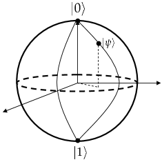
(b) Qubits: states are $\alpha|0\rangle+\beta|1\rangle$ with $\left|{\alpha}\right|^{2}+\left|{\beta}\right|^{2}=1$.

Figure 3: Visualization of bits versus qubits.

The quantum mechanical manipulations of qubits are carried out by operators. For example, the $\mathsf{NOT}$ gate operates on $\alpha|0\rangle+\beta|1\rangle$ to exchange the two logic states:

$$\mathsf{NOT}(\alpha|0\rangle+\beta|1\rangle)=\alpha|1\rangle+\beta|0\rangle.$$ (6)

Similar to quantum states represented by vectors in Eq (5), we can represent operators by matrices. In matrix representation, the $\mathsf{NOT}$ operator is equivalent to $\left[\begin{array}[]{cc}0&1\\ 1&0\end{array}\right]$.

A qubit lives in a Hilbert space. The Hilbert space for several qubits is the tensor product of Hilbert spaces for individual qubits. The notation of tensor product is $\otimes$. Similarly, an aggregate of operators acting on the tensor product of qubits can be represented by the tensor product of individual operators. For the details about quantum mechanics see standard textbooks Griffiths2002-ConsistentQuantTh ; Liboff2003-QuantMech ; Griffiths2005-QuantMech .

Since qubits behave totally differently from classical bits, Nielsen and Chuang NielsenChuang2000-QCQI summarize three difficulties in quantum error correction:

1. Measurement destroys quantum information: Observation in quantum mechanics generally destroys the quantum state under observation, and makes recovery impossible.

2. No cloning: The no-cloning theorem WootersZurek1982-NonCloning states that there is no quantum operation taking a state $|\psi\rangle$ to $|\psi\rangle\otimes|\psi\rangle$ for all states $|\psi\rangle$. In other words, we cannot design a repetition code by duplicating a state several times.

3. Errors are continuous: Since a qubit is continuous, different errors on a single qubit form a continuum. We hence require infinite precision to determine which error occurred in order to correct it.

To overcome the first difficulty, we have to recall lessons from classical error-correcting codes. We would like to use the syndrome in the decoding procedure. Measuring the syndrome alone will not bother the information-carrying quantum states.

The second difficulty can be circumvented by embedding the physical basis $\{|0\rangle,|1\rangle\}$ into a logical basis $\{|0_{L}\rangle,|1_{L}\rangle\}$ of code space:

$$|0\rangle \rightarrow |0_{L}\rangle$$ (7)

$$|1\rangle \rightarrow |1_{L}\rangle\>.$$ (8)

That is, an encoder maps a state $|\psi\rangle=\alpha|0\rangle+\beta|1\rangle$ to $\alpha|0_{L}\rangle+\beta|1_{L}\rangle$. For example, we can encode a message in the sense of a repetition code by

$$|0_{L}\rangle \equiv |000\rangle$$ (9)

$$|1_{L}\rangle \equiv |111\rangle\>.$$ (10)

In the example of Shor code Shor1995-RedDecoherence , the encoded basis is

$$|0_{L}\rangle\equiv\frac{(|000\rangle+|111\rangle)(|000\rangle+|111\rangle)(|000\rangle+|111\rangle)}{2\sqrt{2}}$$ (11)

$$|1_{L}\rangle\equiv\frac{(|000\rangle-|111\rangle)(|000\rangle-|111\rangle)(|000\rangle-|111\rangle)}{2\sqrt{2}}\>.$$ (12)

The third challenge can be dealt with using the fact that any operator on the space of one qubit can be written as a linear combination of Pauli operators defined as:

$$I=\left[\begin{array}[]{cc}1&0\\ 0&1\end{array}\right],\quad\sigma_{x}=\left[\begin{array}[]{cc}0&1\\ 1&0\end{array}\right],$$ (17)

$$\sigma_{z}=\left[\begin{array}[]{cc}1&0\\ 0&-1\end{array}\right],\quad\sigma_{y}=\left[\begin{array}[]{cc}0&-i\\ i&0\end{array}\right]=i\sigma_{x}\sigma_{z}\>.$$ (22)

These operators have effects on the qubit listed in Table 2 Gottesman2000-IntroQuantECC . As long as the decoder can correct errors of $\sigma_{x}$, $\sigma_{y}$, and $\sigma_{z}$, it will correct any and all errors.

Table 2: The Pauli operators.

Identity	$I=\left[\begin{array}[]{cc}1&0\\ 0&1\end{array}\right]$	$I|a\rangle=|a\rangle$
Bit Flip	$\sigma_{x}=\left[\begin{array}[]{cc}0&1\\ 1&0\end{array}\right]$	$\sigma_{x}|a\rangle=|a\oplus 1\rangle$
Phase Flip	$\sigma_{z}=\left[\begin{array}[]{cc}1&0\\ 0&-1\end{array}\right]$	$\sigma_{z}|a\rangle=(-1)^{a}|a\rangle$
Bit and Phase Flip	$\quad\sigma_{y}=\left[\begin{array}[]{cc}0&-i\\ i&0\end{array}\right]=i\sigma_{x}\sigma_{z}\quad$	$\sigma_{y}|a\rangle=i(-1)^{a}|a\oplus 1\rangle\quad$

III.2 Quantum Error Models

Error models in quantum communication are more complex than the binary symmetric channel in classical communication. We now introduce error models by starting with a model for a quantum communication system, as shown in Fig 4. Let the quantum information of interest be a ket $|\psi\rangle$ in a Hilbert space $\mathcal{H}_{A}$. Like adding the redundant bits in classical coding, we consider ancillary qubits in quantum communication. Ancillas are in the Hilbert space $\mathcal{H}_{B}$ and are initially in a definite state $|\bar{b}\rangle$. Usually $|\bar{b}\rangle$ is set to be $|00\cdots 0\rangle$. In the encoding step, an encoder $E$ is a unitary transformation mapping $\mathcal{H}_{C}=\mathcal{H}_{A}\otimes\mathcal{H}_{B}$ to itself. That is, $E(|\psi\rangle\otimes|\bar{b}\rangle)=|c\rangle\in\mathcal{H}_{C}$. $\mathcal{H}_{C}$ is called code space.

Figure 4: Block diagram of a quantum communication system.

With reference to Fig 4, errors in the channel are induced by an interaction between $\mathcal{H}_{C}$ and environment $\mathcal{H}_{N}$ that has initial state $|\bar{n}\rangle$. The effect of this interaction on $\mathcal{H}_{C}$ is represented by a collection $\mathfrak{N}$ of noise operators $\{N_{0}=I,N_{1},N_{2},\cdots\}$ mapping the code $\mathcal{H}_{C}$ to itself. These operators can always be chosen to be linearly independent. The operator $I$ in the collection $\mathfrak{N}$ is an identity map. The effect of the interaction is represented in the operator sum formalism

$$\rho\rightarrow\mathfrak{N}(\rho)\triangleq\sum_{i}N_{i}\rho N_{i}^{\dagger},$$ (23)

where the normalization condition

$$\sum_{i}N_{i}^{\dagger}N_{i}=I$$ (24)

ensures that $\mbox{Tr}\left[\mathfrak{N}(\rho)\right]=1$. There is an orthonormal basis $\{|n_{i}\rangle\}$ on $\mathcal{H}_{N}$ such that for any $|c\rangle$ the corrupted codeword is produced by a mapping

$$|c\rangle\otimes|\bar{n}\rangle\rightarrow\sum_{i}(N_{i}|c\rangle)\otimes|n_{i}\rangle\>.$$ (25)

In the decoding step, a decoder $D$ maps the noise corrupted codeword $|c^{\prime}\rangle$ back to $|\psi\rangle\otimes|s\rangle$, where $|\psi\rangle$ is the message we want to retrieve, and $|s\rangle$ is the syndrome we will use to correct errors. Following the rationale in classical error correction, we want to relate syndromes $|s_{i}\rangle$ to errors $N_{i}$ homomorphically, and hope $|s_{i}\rangle$ is independent of $|\psi\rangle$ for all $|\psi\rangle$ in $\mathcal{H}_{A}$. In short, we should design an encoding/decoding scheme to reach a situation

$$DN_{i}E(|\psi\rangle\otimes|\bar{b}\rangle)=|\psi\rangle\otimes|s_{i}\rangle\>.$$ (26)

Note that any operator can be written as a linear combination of Pauli operators. In order to correct all kinds of errors, the decoder should be able to correct errors of types $\sigma_{x}$, $\sigma_{y}$, and $\sigma_{z}$, listed in Table 2. The quantum error models are apparently more complicated than the classical error model of independent bit flips. To protect the codewords against these noise operators, we next discuss the conditions of error correctability.

III.3 Conditions of Quantum Error Correction

Similar to classical error correction, the procedure of quantum decoding also consists of two steps: error detection and error correction. In the detection step, we want to distinguish different errors in the corrupted codewords. Then we apply the inverse of the error operators in the correction step. If there are error operators corrupting different codewords into an identical codeword, we face ambiguity. In the sequel, the errors to be correctable must meet some conditions.

The condition of quantum error correction is stated in the following theorem KnillLaflamme1997-TheoryQECC :

Theorem 3

Let $\mathcal{H}_{C_{0}}$ be a quantum code and $P$ be the projector onto $\mathcal{H}_{C_{0}}$. A set $\mathfrak{N}_{\mbox{\scriptsize{cr}}}$ of noise operators $\{N_{i}\}$ is correctable if and only if for all $i,j$

$$PN_{i}^{\dagger}N_{j}P=\lambda_{ij}P$$ (27)

for some set of complex numbers $\{\lambda_{ij}\}$.

Theorem 3 can be stated in terms of the orthonormal basis of $\mathcal{H}_{C_{0}}$. Let $\{|c_{q}\rangle\}$ be an orthonormal basis of codewords which span the subspace $\mathcal{H}_{C_{0}}$. Then we have

$$P|c_{q}\rangle=|c_{q}\rangle\quad\mbox{and}\quad(I-P)|c_{q}\rangle=0.$$ (28)

Substituting this relation into Eq (27) gives

$$\langle c_{p}|N_{i}^{\dagger}N_{j}|c_{q}\rangle=\lambda_{ij}\delta_{pq}\>,$$ (29)

which is an equivalent statement to Theorem 3. There are some insights for this theorem. We address them in the following.

1. Only some noise operators are correctable. Recall a lesson in classical error correction: not all the errors are correctable, and the correctable errors depend on the decoding scheme. This means that we do not have an ambition to correct all the error operators in $\mathfrak{N}$, but do focus only on a set $\mathfrak{N}_{\mbox{\scriptsize{cr}}}$ of correctable errors. Since $\mathfrak{N}_{\mbox{\scriptsize{cr}}}$ depends upon the decoding method $D$, we can relate them as $\mathfrak{N}_{\mbox{\scriptsize{cr}}}(D)$. Note that for a given codeword space $\mathcal{H}_{C_{0}}$, there may be more than one possible $D$ and more than one possible family $\mathfrak{N}_{\mbox{\scriptsize{cr}}}$ of correctable errors. Conversely, given some decoding operation $D$, if $\{N_{i}\}$ is any collection of operators drawn from $\mathfrak{N}_{\mbox{\scriptsize{cr}}}(D)$, then Theorem 3 will be satisfied. When Eq (27) holds, the basis states $\{|c_{q}\rangle\}$ span a quantum error-correcting code.

2. Linear space of noise operators. The noise operators $\{N_{i}\}$ in the set $\mathfrak{N}_{\mbox{\scriptsize{cr}}}$ span a linear space $\mathcal{N}$ of operators. We next would like to know whether all the elements in $\mathcal{N}$ are correctable. If $U$ is a matrix (not necessarily unitary) with entries $u_{mn}$, one can define the new noise operators $F_{j}=\sum_{i}u_{ji}N_{i}$. The left hand side of Eq (27) becomes

   $$PF_{i}^{\dagger}F_{j}P = P\left(\sum_{m,n}u_{im}^{*}N_{m}^{\dagger}u_{jn}N_{n}\right)P$$ (30)

   $$= \sum_{m,n}u_{im}^{*}\lambda_{mn}u_{jn}P$$

   $$= (U^{\dagger}\Lambda U)_{ij}P\>,$$

   where $\Lambda$ denotes the matrix $\lambda_{mn}$. Equation (30) shows that all the elements in $\mathcal{N}$ are correctable. That is, if $N_{i}$ and $N_{j}$ are correctable, so is $\alpha N_{i}+\beta N_{j}$. Let $\mathfrak{N}_{\mbox{\scriptsize{cr}}}^{\mbox{\scriptsize{B}}}=\{N_{1}^{\mbox{\scriptsize{B}}},\cdots,N_{M}^{\mbox{\scriptsize{B}}}\}$ be a basis of $\mathcal{N}$. It follows that $\mathfrak{N}_{\mbox{\scriptsize{cr}}}^{\mbox{\scriptsize{B}}}$ satisfies Eq (30) with $F_{i}=N_{i}^{\mbox{\scriptsize{B}}}$.

3. Principal errors. There is a unitary transformation $U$ which can diagonalize the Hermitian matrix $\Lambda$, i.e.,

   $$\lambda_{ij}=\sum_{k}u_{ik}d_{k}u_{jk}^{*}$$ (31)

   with eigenvalues $d_{k}\geq 0$. This is equivalent to defining a new set of error operators $\{F_{k}\}$ such that

   $$PF_{k}^{\dagger}F_{l}P=\delta_{kl}d_{k}P\>.$$ (32)

   For the case of $d_{k}>0$, we define principal errors $V_{k}$ as

   $$V_{k}\triangleq\frac{1}{\sqrt{d_{k}}}F_{k}$$ (33)

   by normalizing $F_{k}$. It follows that $PV_{k}^{\dagger}V_{l}P=\delta_{kl}P$, or equivalently

   $$\langle c_{p}|V_{k}^{\dagger}V_{l}|c_{q}\rangle=\delta_{kl}\delta_{pq}\>.$$ (34)

   Equation (34) is of significance. We first denote $V_{l}|c_{q}\rangle$ as $|c_{q}^{l}\rangle$. When $k\neq l$, Eq (34) reveals that $\mathcal{H}_{C_{k}}$ and $\mathcal{H}_{C_{l}}$ are mutually orthogonal. When $k=l$, Eq (34) becomes $\langle c_{p}^{k}|c_{q}^{k}\rangle=\delta_{pq}$. This means that $V_{k}$ unitarily transforms the codeword space $\mathcal{H}_{C_{0}}$ spanned by $\{|c_{q}\rangle\}$ onto another subspace $\mathcal{H}_{C_{k}}$ spanned by $\{|c_{q}^{k}\rangle\}$.

4. Null errors. In general, some of $d_{k}$ in Eq (31) are zero. The null errors are errors with $d_{k}=0$ such that Eq (32) becomes $PF_{k}^{\dagger}F_{k}P=0$, or, equivalently,

   $$\langle c_{q}|F_{k}^{\dagger}F_{k}|c_{q}\rangle=0\>.$$ (35)

   Since $F_{k}$ are not zero, the role of $F_{k}$ is to annihilate codewords and never contributes a component to the actual state of the system. This simply means that these $F_{k}$ occur with zero probability.

IV Fault-Tolerant Quantum Computation

We have described quantum error correction. However, the computations used during encoding and decoding are vulnerable to errors. In the classical computer systems, the basic idea of fault-tolerant computation is to add spatial redundancy to reduce the probability of failure. This concept applies to fault-tolerant quantum computation as well.

Fig. 5 is an example of Controlled-NOT ($\mathsf{CNOT}$) gate followed by an operation $U$. Unfortunately, there is an error (denoted by $\mathsf{x}$) at one of the inputs of $\mathsf{CNOT}$ gate. The propagation of this error through $\mathsf{CNOT}$ gate generates a catastrophe because $U$ operates on the wrong inputs. To avoid spreading errors through a quantum circuit, we have to scrutinize the behavior of error propagation and design fault-tolerant quantum computation in a systematic way.

Figure 5: An error (denoted by $\mathsf{x}$) at the top input of $\mathsf{CNOT}$ gate propagating through the $\mathsf{CNOT}$ gate results in that $U$ operates on the wrong inputs.

IV.1 The Laws of Fault-Tolerant Quantum Computation

Preskill Preskill1998-ReliableQC ; Preskill1998-FTQC studied quantum error behavior and distilled five laws to design fault-tolerant quantum computation. We summarize them in this section.

1. Do not use the same qubit twice. We use an example in Fig. 6(a) to illustrate this law. In Fig. 6(a), the data consists of two qubits and the ancilla is one qubit. If there is an error in the ancilla, this error will spread catastrophically to the entire circuit. Note that quantum errors can be a bit flip, a phase flip, or a combination. A bit flip error in a $\mathsf{CNOT}$ circuit propagates from the source to the target. A phase error, however, goes in the opposite direction, from the target to the source. The improvement of this circuit is to decompose the ancilla into two qubits, as shown in Fig. 6(b). The new design guarantees that an error in one of the ancilla qubits only affects the circuit once.

   (a) Bad circuit.

   (b) Good circuit.

   Figure 6: Do not use the same bit twice.

2. Copy the errors, not the data qubits. We want to copy onto the ancilla the information about the errors in the data qubits, without inducing additional errors into the data. To achieve this goal, we must prepare an appropriate state of the ancilla before we copy any information. This ancillary state is carefully chosen so that by measuring the ancilla we acquire only information about the errors having occurred, and don’t perturb the encoded data.

3. Verify when we encode a known quantum state. The encoding process is vulnerable to errors—the power of the code to protect against channel noises is not yet in place. A single error may propagate virulently, as we saw in Fig. 6. Therefore, we should carry out a measurement which checks that the encoding has been done correctly.

4. Repeat operations. Operations, such as encoding verification and syndrome measurement, themselves may be erroneous. For instance, errors while measuring a syndrome can both damage the data and generate an erroneous syndrome. Thus we have to repeat an operation to increase our confidence that the operation was performed correctly.

5. Use the right codes. The code we use for computation should have special properties so that we can apply quantum gates to the encoded information that operate efficiently and that adhere to the preceding four laws. For example, a good code for computation might be such that a $\mathsf{CNOT}$ gate acting on encoded qubits is implemented as in Fig. 7 —with a single $\mathsf{CNOT}$ gate applied to each bit in both the source block and the target block.

   Figure 7: Bitwise implementation of a $\mathsf{CNOT}$ gate.

IV.2 Concatenated Codes

These five laws provide a guideline to ensure fault-tolerant quantum computation. In short, we spend spatial resources to reduce failure rate. Figs. 6 and 7 have demonstrated this concept. Besides making quantum computation reliable, another goal of fault-tolerant quantum computation is to build a scalable quantum information processor. The accuracy threshold theorem shows how to achieve these goals. The accuracy threshold theorem Knill1996-ThreAccuracy states the following:

Theorem 4

If the error rate per qubit is less than a threshold, then an arbitrarily long quantum computation can be executed with high reliability.

A feasible realization of Theorem 4 is concatenated codes Knill1996-ConcaQuantCode . A concatenated code is obtained by repeating the following construction several times until a tolerated error rate is achieved. The procedure for constructing a concatenated code is in the following. Suppose we have an error-correcting code $\mathcal{C}$ with size $[m,1]$; i.e., encoding one information qubit into $m$ qubits. In fact, if we magnify these $m$ qubits, every qubit is not really a single qubit but another block of $m$ qubits acquired by encoding this qubit via the same code $\mathcal{C}$. In other words, we actually encode the information qubit into $m^{2}$ qubits. If we again use the code $\mathcal{C}$ to encode each qubit in the second layer to obtain the third level, we essentially encode the initial information qubit into $m^{3}$ qubits. If there are $L$ levels, the information qubit is encoded in a block of $m^{L}$ qubits. This procedure is called concatenation, illustrated in Fig. 8. Note that we have spent more spatial resources (circuit area) to encode one information qubit. However, we don’t increase the complexity of the code $\mathcal{C}$, because, no matter in which layer the code is used, we just build up a hierarchial coding architecture by systematically coping many times the fundamental circuit of $\mathcal{C}$.

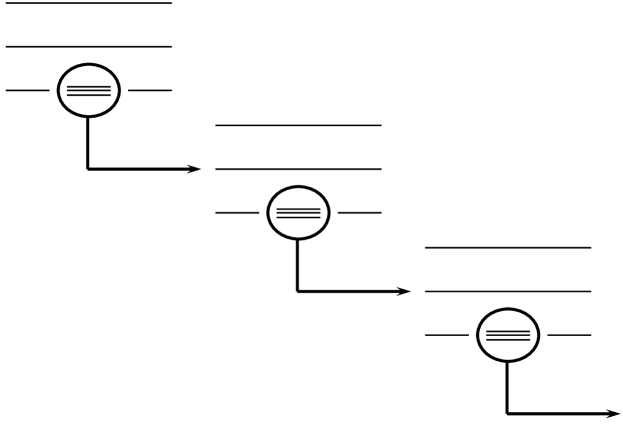
Figure 8: The idea of concatenated codes.

Next, we have to study the performance of using concatenation, to ensure the method provides a better protection. Suppose that the errors are independent events and the probability of error per qubit is $p$. If the code $\mathcal{C}$ is able to correct errors in $g$ of the $m$ qubits, the total probability of recovery failure is

$$\mbox{Pr}_{1}(\epsilon)=\sum_{i=g+1}^{m}\gamma_{i}p^{i}\>,$$ (36)

where the coefficient $\gamma_{i}$ captures the combinatorial effects for the occurrence of $i$ errors. If $p$ is small enough, $\mbox{Pr}_{1}(\epsilon)$ can be bounded as

$$\mbox{Pr}_{1}(\epsilon)\leq\Gamma p^{g+1}$$ (37)

by introducing a constant $\Gamma$. Now we consider a concatenation code with two levels. Recall that there are $m$ sub-blocks of size $m$ qubits. This two level coding architecture fails to correct errors only when there are uncorrectable errors (more than $g$ errors) in more than $g$ sub-blocks. In this case, the probability of failure is

$$\mbox{Pr}_{2}(\epsilon)\leq(\Gamma p^{g+1})^{g+1}\>.$$ (38)

If we use an $L$-level concatenation code, the failure rate reduces to

$$\mbox{Pr}_{L}(\epsilon)\leq\Gamma^{(g+1)^{L-1}}p^{(g+1)^{L}}\>.$$ (39)

Note that Eq (39) is an $L$-fold exponentially decreasing function of $L$. This explains why the concatenation is efficient in reducing the failure rate.

Finally, we use a simple example to illustrate the concatenated codes. Fig. 9 is a case of $\mathsf{CNOT}$ gate with three levels of concatenation. In the first level, we have a generic $\mathsf{CNOT}$ gate. In the second level, each wire is decomposed into two wires; the first-level $\mathsf{CNOT}$ gate now is implemented by two pairs of sub-$\mathsf{CNOT}$ gates. To obtain the third level, each wire in the second level is split into two wires. Now the four pairs of sub-$\mathsf{CNOT}$ gates aggregately perform as a single $\mathsf{CNOT}$ gate in the first level. By creating one more level, we can reduce the probability of failure significantly. In fact, there is no free lunch for reducing failure rate, because we already increase the circuit area and complicate the circuit, as Fig. 9 shows.

Figure 9: $\mathsf{CNOT}$ gate with three levels of concatenation.

V Conclusions

This report investigates the fundamentals of quantum error-correcting codes. The difference between quantum and classical communication systems results from the different characteristics of bits and qubits and from different error models for the noisy channels. Nevertheless, quantum error correction shares many concepts with its classical counterpart. Both quantum and classical coding schemes add ancillary qubits/bits and measure a syndrome to protect information messages. They also have similar conditions for errror detectability and correctability. Due to lack of time, this report leaves out the construction of quantum error-correcting codes, which is now based on Gottesman’s stabilizer codes Gottesman1997-PhD .

The research in quantum error-correcting codes has already migrated to nonbinary codes Rains1999-Nonbinary . However, there is still a long ways to go. In order to use ancillary bits efficiently, modern classical coding theory already goes beyond linear codes. The codes frequently used in practice are nonlinear codes, such as tree codes, trellis codes, turbo codes, and low-density parity-check codes. The nonlinear version of quantum codes is still waiting exploration.

In addition, the typical size of classical codes in usage is $[m=2^{40},k=2^{20}]$, which is unreachable by contemporary quantum codes and fault-tolerant quantum computation. To design a scalable system of quantum information processing, we expect more innovation in the future. Quantum error correction is still in its toddler stage, but we believe that the 21st century will be the golden age of quantum error correction.

References

- (1) C. H. Bennett and P. W. Shor, “Quantum information theory,” IEEE Trans. Inform. Theory, vol. 44, no. 6, pp. 2724–2742, 1998.
- (2) R. E. Blahut, Theory and Practice of Error Control Codes. New York, NY: Addison Wesley, 1983.
- (3) D. Gottesman, “Stabilizer codes and quantum error correction,” Ph.D. dissertation, California Instiute of Technology, Pasadena, CA, 1997, arXiv: quant-ph/9705052.
- (4) ——, “An introduction to quantum error correction,” in Proc. Symp. App. Math., 2000, arXiv: quant-ph/0004072.
- (5) D. J. Griffiths, Introduction to Quantum Mechanics, 2nd ed. Upper Saddle River, NJ: Prentice-Hall, 2005.
- (6) R. B. Griffiths, Consistent Quantum Theory. Cambridge, UK: Cambridge University Press, 2002.
- (7) R. Hamming, “Error-detecting and error-correcting codes,” Bell Syst. Tech. J., vol. 29, pp. 147–160, 1950.
- (8) E. Knill and R. Laflamme, “Concatenated quantum codes,” Los Alamos National Laboratory, Tech. Rep. LAUR-96-2808, 1996.
- (9) ——, “A theory of quantum error-correcting codes,” Phys. Rev. A, vol. 55, pp. 900–911, 1997, arXiv: quant-ph/9604034.
- (10) E. Knill, R. Laflamme, A. Ashikhmin, H. Barnum, L. Viola, and W. H. Zurek, “Introduction to quantum error correction,” Los Alamo Science, no. 27, pp. 188–221, 2002, arXiv: quant-ph/0207170.
- (11) E. Knill, R. Laflamme, and W. H. Zurek, “Threshold accuracy for quantum computation,” Los Alamos National Laboratory, Tech. Rep. LAUR-96-2199, 1996.
- (12) R. L. Liboff, Introductory Quantum Mechanics, 4th ed. San Francisco, CA: Addison Wesley, 2003.
- (13) S. Lin and D. J. Costello, Error Control Coding, 2nd ed. Upper Saddle River, NJ: Prentice-Hall, 2004.
- (14) F. J. MacWilliams and N. J. A. Sloane, The Theory of Error Correcting Codes. Amsterdam, The Netherlands: North-Holland, 1977.
- (15) R. J. McEliece, The Theory of Information and Coding, 2nd ed. Cambridge, UK: Cambridge University Press, 2002.
- (16) M. A. Nielsen and I. L. Chuang, Quantum Computation and Quantum Information. Cambridge, UK: Cambridge University Press, 2000.
- (17) J. Preskill, “Fault-tolerant quantum computation,” in Introduction to Quantum Computation and Information, H.-K. Lo, S. Popescu, and T. Spiller, Eds. River Edge, NJ: World Scientific, 1998.
- (18) ——, “Reliable quantum computers,” Proc. R. Soc. London, Ser. A, vol. 454, pp. 385–4110, 1998.
- (19) E. M. Rains, “Nonbinary quantum codes,” IEEE Trans. Inform. Theory, vol. 45, no. 6, pp. 1827–1832, 1999.
- (20) B. Schumacher, “Quantum coding,” Phys. Rev. A, vol. 51, pp. 2738–2747, 1995.
- (21) C. Shannon, “A mathematical theory of communication,” Bell Syst. Tech. J., vol. 27, pp. 379–423, 1948.
- (22) P. W. Shor, “Scheme for reducing decoherence in quantum memory,” Phys. Rev. A, vol. 52, no. 4, pp. R2493–R2496, 1995.
- (23) A. M. Steane, “Error correcting codes in quantum theory,” Phys. Rev. Lett., vol. 77, no. 5, pp. 793–797, 1996.
- (24) W. K. Wooters and W. H. Zurek, “A single quantum cannot be cloned,” Nature, vol. 299, pp. 802–803, 1982.