Efficiency of quantum and classical transport on graphs

Abstract

We propose a measure to quantify the efficiency of classical and quantum mechanical transport processes on graphs. The measure only depends on the density of states (DOS), which contains all the necessary information about the graph. For some given (continuous) DOS, the measure shows a power law behavior, where the exponent for the quantum transport is twice the exponent of its classical counterpart. For small-world networks, however, the measure shows rather a stretched exponential law but still the quantum transport outperforms the classical one. Some finite tree-graphs have a few highly degenerate eigenvalues, such that, on the other hand, on them the classical transport may be more efficient than the quantum one.

I Introduction.

The transfer of information is the cornerstone of many physical, chemical or biological processes. The information can be encoded in the mass, charge or energy transported. All these transfer processes depend on the underlying structure of the system under study. These could be, for example, simple crystals, as in solid state physics Ziman (1972), more complex molecular aggregates like polymers Kenkre and Reineker (1982), or general network structures Albert and Barabási (2002). Of course, there exists a panoply of further chemical or biological systems which propagate information.

There are several approaches to model the transport on these structures. In (quantum) mechanics, the structure, i.e., the potential a particle is moving in, specifies the Hamiltonian of the system, which determines the time evolution. For instance, the dynamics of an electron in a simple crystal is described by the Bloch ansatz Ziman (1972). Hückel’s molecular-orbital theory in quantum chemistry allows to define a Hamiltonian for more complex structures, such as molecules McQuarrie (1983). This is again related to transport processes in polymers, where the connectivity of the polymer plays a fundamental role in its dynamical and relaxational properties Doi and Edwards (1998). There, (classical) transport processes can be described by a master equation approach with an appropriate (classical) transfer operator which determines the temporal evolution of an excitation Kenkre and Reineker (1982); Weiss (1994).

In all examples listed above, the densities of states (DOS), or spectral density, of a given system of size $N$,

$$\rho(\lambda)=\frac{1}{N}\sum_{n=1}^{N}\delta(\lambda-\lambda_{n}),$$

contains the essential informations about the system. Here, the $\lambda_{n}$’s are the eigenvalues of the appropriate Hamiltonian ${\bf H}$ or transfer operator ${\bf T}$. Depending (mainly) on the topology of the system, $\rho(\lambda)$ shows very distinct features. A classic in this respect is the DOS of a random matrix, corresponding to a random graph Mehta (1991). Wigner has shown that for a (large) matrix with (specific) random entries, the eigenvalues of this matrix lie within a semi-circle Wigner (1955). As we will show, distinct features of the DOS also result in very distinct transport properties.

II Transport on graphs.

We start our discussion by considering quantum mechanical transport processes on discrete structures, in general called graphs, which are a collection of $N$ connected nodes. We assume that the states $|j\rangle$, associated with a localized excitation at node $j$, form an orthonormal basis set and span the whole accessible Hilbert space. The time evolution of an excitation initially placed at node $|j\rangle$ is determined by the systems’ Hamiltonian ${\bf H}$ and reads $\exp(-i{\bf H}t)|j\rangle$. The classical transport can be described by a master equation for the conditional probability, $p_{k,j}(t)$, to find an excitation at time $t$ at node $k$ when starting at time $0$ at node $j$. Using also here the Dirac notation for a state at node $j$, the classical time evolution of this state follows from the transfer matrix ${\bf T}$ of the transport process as $\exp({\bf T}t)|j\rangle$. In order to compare the classical and the quantum motion, we identify the Hamiltonian of the system with the (classical) transfer matrix, ${\bf H}=-{\bf T}$, which we will relate later to the (discrete) Laplacian of the graph, see e.g. Farhi and Gutmann (1998); Mülken and Blumen (2005a). The classical and quantum mechanical transition probabilities to go from the state $|j\rangle$ at time $0$ to the state $|k\rangle$ in time $t$ are given by $p_{k,j}(t)\equiv\langle k|\exp({\bf T}t)|j\rangle$ and $\pi_{k,j}(t)\equiv|\alpha_{k,j}(t)|^{2}\equiv|\langle k|\exp(-i{\bf H}t)|j\rangle|^{2}$, respectively.

III Averaged transition probabilities.

Quantum mechanically, a lower bound of the average probability to be still or again at the initially excited node, $\overline{\pi}_{\rm discr}(t)\equiv\frac{1}{N}\sum_{j=1}^{N}\pi_{j,j}(t)$, is obtained for a finite network by an eigenstate expansion and using the Cauchy-Schwarz inequality as, Mülken et al. (2006),

$$\overline{\pi}_{\rm discr}(t)\geq\left|\frac{1}{N}\sum_{n}\ \exp(-i\lambda_{n}t)\right|^{2}\equiv|\overline{\alpha}_{\rm discr}(t)|^{2}.$$ (1)

Note that $|\overline{\alpha}_{\rm discr}(t)|^{2}$ depends only on the eigenvalues of ${\bf H}$ but not on the eigenvectors. As we have shown earlier, especially the local maxima of $\overline{\pi}(t)$ are very well reproduced by $|\overline{\alpha}(t)|^{2}$ and for regular networks, the lower bound is exact Mülken et al. (2006). Therefore, we will use $|\overline{\alpha}_{\rm discr}(t)|^{2}$ in the following to characterize transport processes.

Also classically one has a simple expression for $\overline{p}_{\rm discr}(t)\equiv\frac{1}{N}\sum_{j=1}^{N}p_{j,j}(t)$, see, e.g., Bray and Rodgers (1988),

$$\overline{p}_{\rm discr}(t)=\frac{1}{N}\sum_{n=1}^{N}\ \exp\big{(}-\lambda_{n}t\big{)}.$$ (2)

Again, this result depends only on the (discrete) eigenvalue spectrum of ${\bf T}$ but not on the eigenvectors.

In the continuum limit, Eqs. (1) and (2) can be written as

$$\overline{\pi}(t) \geq \left|\int d\lambda\ \rho(\lambda)\ \exp(-i\lambda t)\right|^{2}\equiv|\overline{\alpha}(t)|^{2}.$$ (3)

$$\overline{p}(t) = \int d\lambda\ \rho(\lambda)\ \exp(-\lambda t),$$ (4)

The explicit calculation of the integrals is easily done using computer algebra systems like MAPLE or MATHEMATICA; in many cases, the integrals can also be found in Gradshteyn and Ryzhik (1980).

IV Efficiency measure of transport on graphs.

Equations (1)-(4) allow to define an efficiency measure (EM) for the performance of the transport on a graph. We stress again, that the EM does not involve any computationally expensive calculations of eigenstates. Rather, only the energy eigenvalues are needed, which are quite readily obtained by diagonalizing H.

By starting with continuous DOS, since those are mathematically easier to handle, we define the (classical) EM of the graph by the decay of $\overline{p}(t)$ for large $t$, where a fast decay means that the initial excitation spreads rapidly over the whole graph. Quantum mechanically, however, the transition probabilities fluctuate due to the unitary time evolution. Therefore, in most cases also $\overline{\pi}(t)$ and $|\overline{\alpha}(t)|^{2}$ fluctuate. Nevertheless, the local maxima of $|\overline{\alpha}(t)|^{2}$ reproduce the ones of $\overline{\pi}(t)$ rather well. We use now the temporal scaling of the local maxima of $|\overline{\alpha}(t)|^{2}$ as the (quantum) EM and denote the envelope of the maxima by ${\rm env}[|\overline{\alpha}(t)|^{2}]$. Similar to the classical case, a fast decay of ${\rm env}[|\overline{\alpha}(t)|^{2}]$ corresponds to a rapid spreading of an initial excitation.

For a large variety of graphs the DOS can be written as

$$\rho(\lambda)\sim(\lambda\lambda_{m}-\lambda^{2})^{\nu},$$ (5)

with $\nu>-1$ and where $\lambda_{m}$ is the maximal eigenvalue (we assumed the minimum eigenvalue to be zero). Since we are interested in the large $t$ behavior, $\overline{p}(t)$ [and also $\overline{p}_{\rm discr}(t)$] will be mainly determined by small $\lambda$ values, such that for $t\gg 1$ we can assume $\rho(\lambda)\sim\lambda^{\nu}$. Than it is easy to show that the classical EM scales as

$$\overline{p}(t)\sim t^{-(1+\nu)}.$$ (6)

This scaling argument for long times is well known throughout the literature, where $2(1+\nu)\equiv d_{s}$ is sometimes called the spectral or fracton dimension, see, e.g., Alexander et al. (1981).

In order to obtain the quantum mechanical scaling for the same DOS, we can use the same scaling arguments. For $t\gg 1$, also $|\overline{\alpha}(t)|^{2}$ [and $|\overline{\alpha}_{\rm discr}(t)|^{2}$] will be mainly determined by the small $\lambda$ values. In fact, for $\rho(\lambda)\sim\lambda^{\nu}$ one has $|\overline{\alpha}(t)|=\overline{p}(t)$. Here, all quantum mechanical oscillations vanish, because we consider only the leading term of the DOS for small $\lambda$. Thus, we furthermore have ${\rm env}[|\overline{\alpha}(t)|^{2}]=|\overline{\alpha}(t)|^{2}$, i.e., the quantum EM reads

$${\rm env}[|\overline{\alpha}(t)|^{2}]\sim t^{-2(1+\nu)}.$$ (7)

Equation (7) can also be directly obtained from Eq. (3) with $\rho(\lambda)\sim\lambda^{\nu}$. Of course, Eqs. (6) and (7) agree with the solution for $\overline{p}(t)$ and ${\rm env}[|\overline{\alpha}(t)|^{2}]$ obtained from the full DOS $\rho(\lambda)\sim(\lambda\lambda_{m}-\lambda^{2})^{\nu}$. The same scaling has been obtained for the decay of temporal correlations in quantum mechanical systems with Cantor spectra Ketzmerick et al. (1992). There, the (full) probability $\overline{\pi}(t)$, which was smoothed over time, was used.

In general, for $\overline{p}(t)\sim t^{-{\cal P}_{\rm cl}}$, the exponent ${\cal P}_{\rm cl}$ determines the classical EM of the graph because larger ${\cal P}_{\rm cl}$ correspond to a faster decay of $\overline{p}(t)$. Quantum mechanically, we may have ${\rm env}[|\overline{\alpha}(t)|^{2}]\sim t^{-{\cal P}_{\rm qm}}$, such that the exponent ${\cal P}_{\rm qm}$ determines the quantum EM of the graph. Since we consider only the local maxima, the actual (fluctuating) probability $\overline{\pi}(t)$ [bounded from below by $|\overline{\alpha}(t)|^{2}$] might drop well below these values, i.e., there are times $t$ at which $\overline{\pi}(t)\ll 1$. However, these values are very localized in time and the overall performance of the quantum transport is best quantified by the scaling of ${\rm env}[|\overline{\alpha}(t)|^{2}]$.

The difference between the classical and quantum EM is given by the factor

$$\Delta{\cal P}(t)\equiv\ln[{\rm env}[|\overline{\alpha}(t)|^{2}]]/\ln[\overline{p}(t)].$$ (8)

For classical and quantum power law behavior $\Delta{\cal P}(t)$ is time-independent and we have $\Delta{\cal P}={\cal P}_{\rm qm}/{\cal P}_{\rm cl}$. Thus, for the DOS given above, with $\nu<\infty$, we get $\Delta{\cal P}=2$, as could be expected from the wave-like behavior of the quantum motion compared to the normal diffusive behavior of the classical motion.

IV.1 Continuous DOS.

Two important examples are connected to scaling. An infinite hypercubic lattice in $d$ dimensions has as eigenvalues $\lambda(\Theta_{1},\dots,\Theta_{d})\equiv\sum_{n=1}^{d}\lambda(\Theta_{n})$, with $\lambda(\Theta_{n})=2-2\cos\Theta_{n}$ and $\Theta_{n}\in[0,2\pi[$. Here, one can calculate explicitly $|\overline{\alpha}(t)|^{2}$ and $\overline{\pi}(t)$ and demonstrate that the local maxima really obey scaling; we get namely $|\overline{\alpha}(t)|^{2}=\overline{\pi}(t)\sim|J_{0}(2t)|^{2d}$ Mülken et al. (2006). For $t\gg 1$ this can be approximated by $\overline{\pi}(t)\sim\sin^{2d}(2t+\pi/4)/t^{d}$ Gradshteyn and Ryzhik (1980). Since the maximum of the $\sin$-function is $1$, the quantum measure scales as ${\rm env}[|\overline{\alpha}(t)|^{2}]={\rm env}[\overline{\pi}](t)\sim t^{-d}$, which is what one also obtains from the scaling argument above and $\rho(\lambda)\sim\lambda^{d/2-1}$. Then $\nu=d/2-1$, and the classical measure scales as $\overline{p}(t)\sim t^{-d/2}$ (i.e., the spectral dimension is $d_{s}=d$).

As a second example, we take a random graph. It was shown that the eigenvalue spectrum of the Laplacian of such a graph obeys Wigner’s semi-circle law Wigner (1955); Mehta (1991), which we obtain for $\nu=1/2$ from the DOS given above. For large times both measures again obey scaling and we have $\overline{p}(t)\sim t^{-3/2}$ and ${\rm env}[|\overline{\alpha}(t)|^{2}]\sim t^{-3}$.

Figure 1 shows the temporal behavior of $\overline{p}(t)$ and $|\overline{\alpha}(t)|^{2}$ as well as the power law behavior of $\overline{p}(t)$ and ${\rm env}[|\overline{\alpha}(t)|^{2}]$ for (a) an infinite, regular, one-dimensional (1D) graph and (b) a random graph. Note that here (and in the following figures, too) the very localized minima of $|\overline{\alpha}(t)|^{2}$ do not always show up clearly in the logarithmic scale used.

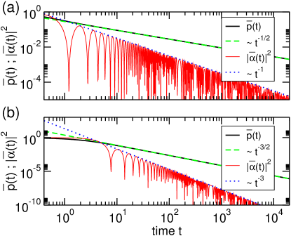
Figure 1: (Color online). $\overline{p}(t)$ and $|\overline{\alpha}(t)|^{2}$ as well as the power laws given in Eqs. (7) and (6) for (a) an infinite regular (1D) graph ($\nu=-1/2$) and (b) a random graph whose DOS obeys Wigner’s semi-circle law ($\nu=1/2$).

For some DOS, the EMs show no power law behavior. The DOS given above are bounded from above by a maximal eigenvalue. This does not have to be the case. The DOS of small-world networks, for instance, may show long $\lambda$-tails Monasson (1999). One additional feature of such DOS is that they do not obey any simple scaling for small $\lambda$. Nevertheless, sometimes analytic solutions for, at least, $\overline{p}(t)$ can be obtained Monasson (1999), as, for example for certain 1D systems with $\rho(\lambda)\sim\lambda^{-3/2}\exp(-1/\sqrt{\lambda})$.

For computational simplicity we consider a 2D system with

$$\rho(\lambda)=\lambda^{-b}\exp(-1/\lambda)$$ (9)

for $\lambda\in[0,\infty[$ and $b>1$. The term $\exp(-1/\lambda)$ is usually referred to as Lifshits tail, while the term $\lambda^{-b}$ assures that $\lim_{\lambda\to\infty}\rho(\lambda)=0$. Then, for $t\gg 1$, the EMs are proportional to the product of a stretched exponential and a power law Gradshteyn and Ryzhik (1980),

$$|\overline{\alpha}(t)|^{2}={\rm env}[|\overline{\alpha}(t)|^{2}] \sim t^{(2b-3)/2}\exp\left(-2\sqrt{2t}\right)$$ (10)

$$\overline{p}(t) \sim t^{(2b-3)/4}\exp\left(-2\sqrt{t}\right).$$ (11)

Furthermore, $\overline{\pi}(t)$ does not oscillate, an effect which is interesting in itself but we will not elaborate on this here.

Although we do not obtain a simple relation between the classical and the quantum EMs, $[\overline{p}(t)]^{2}$ and ${\rm env}[|\overline{\alpha}(t)|^{2}]$ still display similar functional forms. Now, however, $\Delta{\cal P}(t)=[2(2b-3)\ln t-8\sqrt{2t}]/[(2b-3)\ln t-8\sqrt{t}]$ is time-dependent. Equations (11) and (10) are only valid for $t\gg 1$, such that $\lim_{t\to\infty}\Delta{\cal P}(t)=\sqrt{2}$ for all $b$. Hence, also here the quantum transport outperforms the classical one, which is also confirmed by numerical integration of the time-dependent Schrödinger equation for a small-world network Kim et al. (2003). In fact, in both cases the transport is faster than for a regular 2D graph. We note that localization is related to other features of the DOS as we will recall below. However, at intermediate times the quantum EM may drop below the classical EM; the position of the crossover from $\Delta{\cal P}(t)<1$ to $\Delta{\cal P}(t)>1$ depends on the exponent $b$.

IV.2 Discrete DOS.

Up to now, we have only considered continuous DOS, where the quantum EM is quicker than the classical one. In the following we will consider discrete DOS which are obtained by modeling the motion on a given graph classically by continuous-time random walks (CTRWs), see, e.g., Weiss (1994), and quantum mechanically by continuous-time quantum walks (CTQWs) Farhi and Gutmann (1998); Mülken and Blumen (2005a). The Hamiltonian is given by the (discrete) Laplacian associated with the graph, i.e., by the functionality of the nodes and their connectivity. We assume the jump rates between all connected pairs of nodes of the graph to be equal.

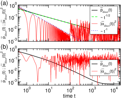
Figure 2: (Color online). $\overline{p}_{\rm discr}(t)$ and $|\overline{\alpha}_{\rm discr}(t)|^{2}$ for (a) a finite regular (1D) graph of size $N=200$ with periodic boundary conditions and (b) a dendrimer of generation $10$ having functionality $z=3$, i.e. $N=3\cdot 2^{10}-2$. Panel (a) contains also the power-law behavior for the infinite regular (1D) graph, see Fig. 1(a).

In general, for finite graphs, $\overline{p}_{\rm discr}(t)$ and ${\rm env}[|\overline{\alpha}_{\rm discr}(t)|^{2}]$ do not decay ad infinitum but at some time will remain constant (classically) or fluctuate about a constant value (quantum mechanically). This time is given by the time it takes for the CTRW to reach the (equilibrium) equipartitioned probability distribution and for the CTQW to fluctuate about a saturation value. At intermediate times, $\overline{p}_{\rm discr}(t)$ and ${\rm env}[|\overline{\alpha}_{\rm discr}(t)|^{2}]$ will show the same scaling as for a system with the corresponding continuous DOS. Figure 2(a) shows the temporal behavior of $\overline{p}_{\rm discr}(t)$ and $|\overline{\alpha}_{\rm discr}(t)|^{2}$ for a finite regular 1D graph of size $N=200$ with periodic boundary conditions, see also Mülken and Blumen (2005b). At intermediate times, the scaling behavior is obviously that of the continuous case shown in Fig. 1(a).

Tree-like graphs do not display scaling in general. For CTQW on hyperbranched structures (like Cayley trees, dendrimers or Husimi cacti), the transition probability between two nodes strongly depends on the site $j$ of the initial excitation Mülken and Blumen (2005a); Mülken et al. (2006). Even in the long time average,

$$\chi_{k,j}=\lim_{T\to\infty}T^{-1}\int_{0}^{T}dt\ \pi_{k,j}(t),$$ (12)

there are transition probabilities which are considerably lower than the equipartitioned classical value Mülken and Blumen (2005a); Mülken et al. (2006). In Fig. 2(b) we display the temporal behavior of $\overline{p}_{\rm discr}(t)$ and $|\overline{\alpha}_{\rm discr}(t)|^{2}$ for a dendrimer of generation $10$ having functionality $z=3$, i.e. $N=3\cdot 2^{10}-2$. Here the classical curve does not show scaling at intermediate times. Quantum mechanically, however, $|\overline{\alpha}_{\rm discr}(t)|^{2}$ has a strong dip at short times but then fluctuates about a finite value which is larger than the classical saturation value. One should also bear in mind that $|\overline{\alpha}_{\rm discr}(t)|^{2}$ is a lower bound and the actual probability will be larger. Therefore, according to our measure for intermediate $t\gg 1$, the classical transport outperforms the quantum transport on these special, finite graphs. As we proceed to show, the reason for this is to be found in the DOS. This is related to (Anderson) localization. Anderson showed that for localization the DOS has to display a discrete finite series of $\delta$ functions Anderson (1978).

We consider now a simple star graph, having one core node and $N-1$ nodes directly connected to the core but not to each other. The eigenvalue spectrum of this star has a very simple structure, there are $3$ distinct eigenvalues, namely $\lambda_{1}=0$, $\lambda_{2}=1$, and $\lambda_{3}=N$, having as degeneracies $g_{1}=1$, $g_{2}=N-2$, and $g_{3}=1$. Therefore we get

$$\overline{p}_{\rm discr}(t) = \frac{1}{N}\left[1+(N-2)e^{-t}+e^{-(N-2)t}\right]$$ (13)

$$\overline{\pi}_{\rm discr}(t) \geq \frac{1}{N^{2}}\left|1+(N-2)e^{-it}+e^{-i(N-2)t}\right|^{2}.$$ (14)

Obviously, only the term $|(N-2)\exp(-it)|^{2}/N^{2}=(N-2)^{2}/N^{2}$ in Eq. (14) is of order ${\cal O}(1)$. All the other terms are of order ${\cal O}(1/N)$ or ${\cal O}(1/N^{2})$ and, therefore, cause only small oscillations (fluctuating terms) about or negligible shifts (constant terms) from $(N-2)^{2}/N^{2}$.

Having only one low lying eigenvalue which is highly degenerate and no other eigenvalue of a degeneracy of the same order of magnitude, results in $\overline{p}_{\rm discr}(t)<\overline{\pi}_{\rm discr}(t)$ for all times $t$ and $\overline{p}_{\rm discr}(t)<|\overline{\alpha}_{\rm discr}(t)|^{2}$ for almost all times $t$. Figure 3 shows the temporal behavior of $\overline{p}_{\rm discr}(t)$, $\overline{\pi}_{\rm discr}(t)$, and $|\overline{\alpha}_{\rm discr}(t)|^{2}$ for $N=10$. Now, for all times, the quantum transport is slower than the classical one. We also see that $|\overline{\alpha}_{\rm discr}(t)|^{2}$ fluctuates about $(N-2)^{2}/N^{2}=16/25$.

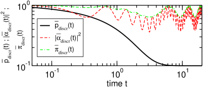
Figure 3: (Color online). $\overline{p}_{\rm discr}(t)$, $\overline{\pi}_{\rm discr}(t)$, and $|\overline{\alpha}_{\rm discr}(t)|^{2}$ for a star with $N=10$.

In general we find for our star-graph that the classical EM is lower than the quantum EM. This result is to some extent also obeyed by dendrimers and by other hyperbranched structures. These, too, have a few highly degenerate eigenvalues, all other degeneracies being an order of magnitude less, which results in the absence of any scaling of ${\rm env}[|\overline{\alpha}_{\rm discr}(t)|^{2}]$, see Fig. 2(b). Of course, the details are much more complex due to the more complex structure, we will elaborate on this elsewhere.

V Conclusion.

We have proposed a measure to classify the efficiency of classical and quantum mechanical transport processes. Depending on the density of states, the quantum transport outperforms the classical transport by means of the speed of the spreding of an initial excitation over a given system. For algebraic DOS, the EMs confirm the difference between classical diffusive and quantum mechanical wave-like transport. Also for small-world networks the quantum mechanical EM is lower than the classical one, i.e. the quantum mechanical transport is faster.

However, for some finite graphs with a few highly degenerate eigenvalues it may happen that the classical transport is more efficient, i.e., that the (quantum) states become localized. We have shown this analytically for a simple star graph. More complex structures, like dendrimers or hyperbranched fractals, show an analogous behavior.

References

- Ziman (1972) J. M. Ziman, Principles of the Theory of Solids (Cambridge University Press, Cambridge, England, 1972); N. W. Ashcroft and N. D. Mermin, Solid State Physics (Saunders College Publishing, Philadelphia, 1976).
- Kenkre and Reineker (1982) V. M. Kenkre and P. Reineker, Exciton Dynamics in Molecular Crystals and Aggregates (Springer, Berlin, 1982); A. S. Davydov, Theory of Molecular Excitons (McGraw-Hill, New York, 1962).
- Albert and Barabási (2002) R. Albert and A.-L. Barabási, Rev. Mod. Phys. 74, 47 (2002); S. N. Dorogovtsev and J. F. F. Mendes, Adv. Phys. 51, 1079 (2002).
- McQuarrie (1983) D. A. McQuarrie, Quantum Chemistry (Oxford University Press, Oxford, 1983).
- Doi and Edwards (1998) M. Doi and S. F. Edwards, The Theory of Polymer Dynamics (Oxford University Press, Oxford, 1998).
- Weiss (1994) N. van Kampen, Stochastic Processes in Physics and Chemistry (North-Holland, Amsterdam, 1990); G. H. Weiss, Aspects and Applications of the Random Walk (North-Holland, Amsterdam, 1994).
- Mehta (1991) M. L. Mehta, Random Matrices (Academic Press, San Diego, 1991); B. Bollobás, Random Graphs (Academic Press, Orlando, 1985).
- Wigner (1955) E. P. Wigner, Ann. Math. 62, 548 (1955).
- Farhi and Gutmann (1998) E. Farhi and S. Gutmann, Phys. Rev. A 58, 915 (1998).
- Mülken and Blumen (2005a) O. Mülken and A. Blumen, Phys. Rev. E 71, 016101 (2005a).
- Mülken et al. (2006) O. Mülken, V. Bierbaum, and A. Blumen, J. Chem. Phys. 124, 124905 (2006); A. Blumen, V. Bierbaum, and O. Mülken, Physica A (2006), accepted.
- Bray and Rodgers (1988) A. J. Bray and G. J. Rodgers, Phys. Rev. B 38, 11461 (1988); A. Blumen, A. Volta, A. Jurjiu, and T. Koslowski, J. Lumin. 111, 327 (2005).
- Gradshteyn and Ryzhik (1980) I. S. Gradshteyn and I. M. Ryzhik, Table of Integrals, Series, and Products (Academic Press, 1980); M. Abramowitz and I. A. Stegun, eds., Handbook of Mathematical Functions (Dover, New York, 1972).
- Alexander et al. (1981) S. Alexander, J. Bernasconi, W. R. Schneider, and R. Orbach, Rev. Mod. Phys. 53, 175 (1981); S. Alexander and R. Orbach, J. Phys. (Paris) Lett. 43, L625 (1982); J. Klafter and A. Blumen, J. Chem. Phys. 80, 875 (1984); S. Havlin and D. Ben-Avraham, Adv. Phys. 36, 695 (1987).
- Ketzmerick et al. (1992) R. Ketzmerick, G. Petschel, and T. Geisel, Phys. Rev. Lett. 69, 695 (1992); J. Vidal, R. Mosseri, and J. Bellissard, J. Phys. A: Math. Gen. 32, 2361 (1999).
- Monasson (1999) R. Monasson, Eur. Phys. J. B 12, 555 (1999); S. Jespersen, I. M. Sokolov, and A. Blumen, Phys. Rev. E 62, 4405 (2000); S. Jespersen and A. Blumen, Phys. Rev. E 62, 6270 (2000).
- Kim et al. (2003) B. J. Kim, H. Hong, and M. Y. Choi, Phys. Rev. B 68, 014304 (2003).
- Mülken and Blumen (2005b) O. Mülken and A. Blumen, Phys. Rev. E 71, 036128 (2005b).
- Anderson (1978) P. W. Anderson, Rev. Mod. Phys. 50, 191 (1978).