Test of nonlocality for a continuos-variable state based on arbitrary number of measurement outcomes

Abstract

We propose a scheme to test Bell’s inequalities for an arbitrary number of measurement outcomes on entangled continuous variable (CV) states. The Bell correlation functions are expressible in terms of phase-space quasiprobability functions with complex ordering parameters, which can experimentally be determined via local CV-qubit interaction. We demonstrate that CV systems can give higher violations of these Bell’s inequalities than of the ones developed for two-outcome observables.

Triggered by research in the foundations of quantum mechanics, in more recent years, new ways of communication and computation were discovered, which are based on quantum laws and can outperform their classical counterparts. From a conceptual point of view one distinguishes quantum information theory based on discrete and continuous variable (CV) quantum systems.

On practical side the use of CVs has an advantage in efficient implementation of the essential steps in quantum information protocols, such as preparing, manipulating and measuring of continuous quadrature amplitudes of the quantized electromagnetic field. CV entanglement can be efficiently produced using squeezed light and measured by homodyne detection Braunstein05 . On the conceptual side the advantage of CV systems over qubits originates in infinite-dimensionality of its Hilbert space. For example, a single CV system may be mapped on a discrete system of arbitrary dimension and hence can be used as a universal resource in the quantum protocols that are based on higher-dimensional systems (qudits) Brukner03 .

The notion of entanglement first appeared explicitly in the literature in 1935, in a CV setting of Einstein, Podolski and Rosen (EPR) EPR35 . They considered an entangled state (the EPR-state)

$$|\mbox{EPR}\rangle\propto\int dx\mbox{ }|x\rangle_{1}\otimes|x-Q\rangle_{2},$$ (1)

of two particles $1$ and $2$ that have perfectly correlated positions ($x_{1}\!-\!x_{2}\!=\!Q$) and momenta $(p_{1}\!+\!p_{2}\!=\!0)$, but is unnormalized. Here $|x\rangle_{1}\otimes|x-Q\rangle_{2}$ denotes a product state of the two particles. The EPR state can be thought of as the limiting case of properly normalized two-mode squeezed vacuum (TMSV) state for infinitely large squeezing. Experimentally, it can be produced by a nondegenerate optical parametric amplifier.

Bell argued that the original EPR state allows a local realistic description in terms of position and momentum because its Wigner function is positive everywhere and hence can serve as a classical probability distribution for local hidden variables Bell87 . Ironically, it was demonstrated that the Wigner function provides a direct evidence of the nonlocal character of the states Banaszek99 , though it does not lead to the maximal violation of Bell’s inequality for the EPR state (the Cirelson’s bound of $2\sqrt{2}$ can not be reached). However, there is no fundamental contradiction between the two statements as in Banaszek99 , the form of the Wigner function merely coincides with the correlation function for parity measurements rather than it is used as the probability function to calculate the correlation. The approach has been generalized by introducing pseudo-generators of SU(d) algebra for CV systems Brukner03 ; Chen02 . It established mathematical equivalence between discrete $d$-dimensional and CV systems, which in principle allows for stronger violation of Bell’s inequalities, but its experimental realization is far beyond the reach of present technology. Thus, as for proposals for revealing the nonlocality of entangled CV states, the current state-of-art suggests that there is a tradeoff between the efficiency and feasibility of the nonlocality tests.

Is it possible to find efficient tests of quantum non-locality for CV systems without compromising too much on their feasibility? In this paper we propose a feasible scheme that allows one to test an arbitrary entangled state of CV systems as if it were a state of a discrete system of arbitrary dimension. This allows to test Bell’s inequalities for arbitrarily high-dimensional systems Collins02 . The measured correlations revealing the nonlocality between higher-dimensional systems are shown to have a natural description in terms of phase-space quasiprobability functions with complex ordering parameters. We demonstrate that CV systems can give higher violation for Bell’s inequalities of larger dimension than for dichotomic observables Banaszek99 . The recent advances in the field of experimental quantum-state manipulation and measurements are shown to provide feasible experimental schemes for measuring quantum correlation functions Lutterbach97 ; Bertet02 .

Generic Bell function for higher dimensional systems- In what follows we will use a generic form of the Bell function for a bipartite $d$ dimension as obtained in Ref. Son05 :

$$\hat{\cal B}=\sum_{n=1}^{d-1}G_{n}\hat{J}_{A}^{n}\otimes\hat{J}_{B}^{n}+h.c.$$ (2)

where the $n$-th order higher spin annihilation operators $\hat{J}_{A}^{n}$ and $\hat{J}_{B}^{n}$ are given as $\hat{J}_{A}^{n}=\frac{1}{2}(\hat{A}_{1}^{n}+\omega^{n/2}\hat{A}_{2}^{n})$ and $\hat{J}_{B}^{n}=\frac{1}{2}(\hat{B}_{1}^{n}+\omega^{n/2}\hat{B}_{2}^{n})$. In the construction of the annihilation operators, the measurement operators $\hat{A}_{i}$ and $\hat{B}_{i}$ represent the measurement on the parties $A$ and $B$ with the measurement settings of $i$. Eigenvalues of the operator $\hat{A}_{i}$ and $\hat{B}_{i}$, which correspond to the measurement outcomes, are assigned by one of complex values $1,\omega,\omega^{2},\cdot\cdot\cdot,\omega^{(d-1)}$ where $\omega=e^{\frac{2\pi i}{d}}$. It is notable that the generic Bell function gives a distinction between quantum and classical statistics when a proper choice of the arbitrary complex coefficient $G_{n}$ is made Son05 .

Due to the cyclic structure of the eigenvalues, the Hermitian conjugate of the measurement operators are given as $(\hat{A}^{\dagger})^{n}=\hat{A}^{(d-n)}$. Together with the Hermitian conjugated part, the Bell operator can be expanded by the measurement operators $\hat{A}$ and $\hat{B}$. Thus, the expectation value of the Bell operator is given as

$$\langle\hat{\cal B}\rangle = \frac{1}{4}\sum_{n=1}^{d-1}\Big{[}f_{n}^{+}\left(\langle\hat{A}_{1}^{n}\hat{B}_{1}^{n}\rangle+\omega^{n}\langle\hat{A}_{2}^{n}\hat{B}_{2}^{n}\rangle\right)$$

$$~{}~{}~{}~{}~{}~{}~{}~{}+f_{n}^{-}\left(\omega^{n/2}\langle\hat{A}_{1}^{n}\hat{B}_{2}^{n}\rangle+\omega^{n/2}\langle\hat{A}_{1}^{n}\hat{B}_{2}^{n}\rangle\right)\Big{]}$$

where $f_{n}^{\pm}\equiv(G_{n}\pm G_{d-n}^{*})$. Each correlation function $\langle\hat{A}_{i}^{n}\hat{B}_{j}^{n}\rangle$ is the function of probabilities for the measurement outcomes. With an antisymmetric match of the outcomes, we have

$$\langle\hat{A}_{i}^{n}\hat{B}_{j}^{n}\rangle = \sum_{k,l=0}^{d-1}\omega^{n(k-l)}P(A_{i}=k,B_{j}=l)$$ (4)

$$= \sum_{m=0}^{d-1}\omega^{nm}P(A_{i}-B_{j}\doteq m)$$

where $P(A_{i}=k,B_{j}=l)$ is the probability that each party obtains the measured outcomes $k$ and $l$ from the measurement $(A_{i},B_{j})$. $P(A_{i}-B_{j}\doteq m)$ is the probability that the difference of the outcomes $(k,l)$ is equal to $m$ modulo $d$. The second equality is followed because $\omega^{k}$ has the same value for same $k$ modulo $d$.

With a proper choice of $f_{n}^{\pm}$, the classical expectation value of the Bell function in Eq. (Test of nonlocality for a continuos-variable state based on arbitrary number of measurement outcomes), under the local realistic theory, is bounded by a certain value that is violated by a quantum state. Interestingly, Collins-Gisin-Linden-Massar-Popescu (CGLMP) inequality Collins02 which is known as tight Bell inequality Masanes02 for a bipartite $d$-dimensional system can also be derived from it. As a non-trivial simplest case, the CGLMP function for $d=3$ is

$$I_{3} = [P(A_{1}-B_{1}\doteq 0)-P(A_{1}-B_{1}\doteq 1)]$$

$$-[P(A_{2}-B_{2}\doteq 0)-P(A_{2}-B_{2}\doteq 2)]$$

$$+[P(A_{1}-B_{2}\doteq 0)-P(A_{1}-B_{2}\doteq 2)]$$

$$+[P(A_{2}-B_{1}\doteq 0)-P(A_{2}-B_{1}\doteq 2)]$$

which is equivalent to the Bell function (Test of nonlocality for a continuos-variable state based on arbitrary number of measurement outcomes) with $f^{+}_{n}=\frac{4}{1-\omega^{n}}$ and $f^{-}_{n}=-\frac{4\omega^{n/2}}{1-\omega^{n}}$. Through its generalization, one can show that, by setting the coefficient function $f^{\pm}_{n}$ as

$$f^{\pm}_{n} = \pm\frac{4}{d}\sum_{k=0}^{d-1}\left(\frac{2k}{d-1}-1\right)\omega^{-\left(k+\frac{3\pm 1}{4}\right)n}$$ (6)

the Bell function in Eq. (Test of nonlocality for a continuos-variable state based on arbitrary number of measurement outcomes) becomes CGLMP function for arbitrary $d$ footnote . The function is proven to be bounded by maximum value $2$ for any classical expectation value, i.e. $\langle\hat{\cal B}\rangle\leq 2$. In general, an arbitrary correlation can be considered with a choice of $f_{n}^{\pm}$. However, in the rest of our paper, we will only consider the CGLMP inequality for our nonlocality test since it is tight for a bipartite $d$-dimensional case. For the nonlocality test, we investigate a way to measure the correlation (4).

Measurement of the complex observable for a CV state- One can ask how the complex observable is measured in a real experimental setup. It is possible if one measures the $d$-level system by discriminating all the $d$ outcomes and assign the corresponding complex values for the measured outcomes. A CV state is possible to be measured by a $d$ outcome measurement, if there is a measurement that makes an arbitrary high dimensional system projected onto a $d$-dimensional subspace Brukner03 . For this purpose, we introduce a $d$-modulo observable

$$\hat{O}_{\alpha}=\hat{D}(\alpha)\sum_{n=0}^{\infty}e^{2in\pi/d}|n\rangle\langle n|\hat{D}^{\dagger}(\alpha),$$ (7)

where the displacement operation $\hat{D}(\alpha)=\exp(\alpha\hat{a}-\alpha^{*}\hat{a}^{\dagger})$ Cahill69 , with bosonic annihilation $\hat{a}$ and creation $\hat{a}^{\dagger}$ operators, is a feasible unitary operation for a CV state Banaszek99 . The observable (7) maps every possible number states $|n\rangle$ into $d$-modulo complex numbers in a unit circle and its expectation value for a state of density operator $\hat{\rho}$ is

$$\langle\hat{O}_{\alpha}\rangle=\sum_{n=0}^{\infty}\left(\frac{z+1}{z-1}\right)^{n}\langle n|\hat{D}^{\dagger}(\alpha)\hat{\rho}\hat{D}(\alpha)|n\rangle$$ (8)

where $z=-i\cot\pi/d$. It is interesting to note that the expectation value of the complex observable (7) is proportional to the quasiprobability function $W(\alpha,z)$ whose ordering parameter can be shown to be a complex number $z$ (see Ref. Cahill69 ):

$$\langle\hat{O}_{\alpha}\rangle=\frac{\pi(1-z)}{2}~{}W(\alpha,z).$$ (9)

One noticeable difference from a usual quasiprobability function frequently considered in quantum optics is that ‘$z$’ is complex instead of real. When $z=0$, the case reduces to the dichotomic measurement Banaszek99 and the expectation value for the observable is proportional to the Wigner function Cahill69 . The expectation value (8) can be reconstructed by optical tomography Vogel89 . Au contraire, the observable (7) has also been measured directly Lutterbach97 ; Bertet02 for $d=2$, using atomic interferometry and dispersive atom-field interaction. A two-level atom (a qubit device) initially prepared in its ground state passes through three interaction zones with the centre zone being the interaction with the field whose even or odd parity is to be measured. In the first and last interaction zones, the atom interacts with external fields for atomic state rotation, $\hat{R}_{i}={1\over\sqrt{2}}\openone+{i\over\sqrt{2}}(\sin\varphi_{i}\hat{\sigma}_{x}+\cos\varphi_{i}\hat{\sigma}_{y})$. Here, $\hat{\sigma}_{x,y,z}$ are Pauli spin operators and $\varphi_{i}$ ($i=1,3$ represents the interaction zone) is determined by the phase of the external field. In the center zone, the evolution is arranged for the atom-field evolution operator is described by $\hat{U}=\exp[i{\phi\over 2}\openone+i(\hat{n}+{1\over 2})\hat{\sigma}_{z})]$, where $\hat{n}=\hat{a}^{\dagger}\hat{a}$ and $\phi$ is the interaction parameter. After passing through the interaction zones, the atom is measured in its excited or ground state. Considering only the relevant terms, the field-atom state at the atomic measurement is Lutterbach97

$$|g\rangle\langle g|\otimes\hat{M}_{-}\hat{\rho}\hat{M}_{-}+|e\rangle\langle e|\otimes\hat{M}_{+}\hat{\rho}\hat{M}_{+},$$ (10)

where $\hat{M}_{\pm}=1\pm\mbox{e}^{i(2\hat{n}+1)\phi+i\eta}$, $\eta=\varphi_{2}-\varphi_{1}$ and $|g,e\rangle$ represent the atomic ground and excited states. For $\phi=-\eta=\pi/2$, we find that the field in an even (odd) photon-number state is signaled by the atom measured in the excited (ground) state. Recently, this has been realized by an experiment Bertet02 to measure the parity for a displaced Fock state prepared in a cavity. The displacement operation, $\hat{D}(\alpha)$, was performed by driving the cavity by an external field. The atom-field evolution, $\hat{U}$, was implemented by atom-field interaction at non-zero detuning $\delta$ for the time $t_{2}=\frac{\pi\delta}{4\Omega^{2}}$ where $\Omega$ is the Rabi frequency. With use of the relation (9), the Wigner function was measured for the Fock state with deep negativity and detailed fringes. The detection efficiency to discriminate the atomic state is highly efficient while there is a non-negligible chance to miss atoms by a detector. However missing atoms is not a problem in our non-demolition measurement setup and the measurement device can be activated only at a right interaction time. An error in the atomic interaction time is due to the atomic velocity fluctuation around 3%.

Even though the experimental model we have here is based on cavity quantum electrodynamics, this can be done by any physical setup which realizes a type of Ramsey interferometer with the dispersive CV field-qubit interaction. For example, direct measurements of the quantum state have been proposed for the vibrational mode of a trapped ion and an electromagnetic field in a superconducting transmission line Spiller05 .

Since the above scheme is a nondemolition measurement, it can be repeated to perform further measurements. By repeating the procedure for a time $t_{4}={1\over 2}t_{2}$, we can project the field onto the subspaces spanned by $4n$ and $4n+2$, once the first atom projected the field onto the even photon number state (by $4n+1$ and $4n+3$ for the odd photon number state). The method can be applied successively for the $d$ outcomes if $d$ is a power of two but, unfortunately, it does not seem straightforward to generalize this scheme to any measurement outcomes.

If we are experimentally conditioned to have only the expectation value of the observable (instead of the individual measurement outcomes), (8), we can use the scheme above for any number of measurement outcomes. Setting the interaction time $t_{d}={2\over d}t_{2}$ and atoms to interact with the field, then measure the difference ($\Delta_{\eta}=P_{e}-P_{g}$) in the probabilities of the atoms being in the excited ($P_{e}$) and the ground ($P_{g}$) states. Using Eq. (10), we can prove that the difference corresponds to the expectation value:

$$\Delta_{\eta}=-\mbox{Re}\left[e^{i(\eta+\frac{\pi}{d})}\langle\hat{O}(\alpha)\rangle\right].$$ (11)

If we remind that the expectation value is complex-valued, it is required to measure both its real and imaginary parts, which is possible by changing $\eta$ dependent upon the number of outcome $d$ as one can find in Eq.(11).

Measuring the correlation for Bell violation - In order to test the violation of the CGLMP inequality (Test of nonlocality for a continuos-variable state based on arbitrary number of measurement outcomes), we need to measure the correlation $\langle\hat{A}_{i}^{n}\hat{B}_{j}^{n}\rangle$. As we restrict our system to a CV state and the unitary operation to displacement operation $\hat{D}(\alpha)$, the correlation function which has to be measured is $\langle\hat{O}^{n}_{\alpha_{i}}\hat{O}^{n\dagger}_{\beta_{j}}\rangle$. After an arrangement, one can find that the correlation function corresponds to the two-mode quasiprobability function

$$\langle\hat{O}^{n}_{\alpha_{i}}\hat{O}^{n\dagger}_{\beta_{j}}\rangle = \frac{\pi^{2}(1-z_{n}^{2})}{4}W(\alpha_{i},\beta_{j},z_{n})$$ (12)

where

$$W(\alpha_{i},\beta_{j},z_{n})=\sum_{m,l=0}^{\infty}\left(\frac{z_{n}+1}{z_{n}-1}\right)^{m-l}$$ (13)

$$~{}~{}~{}~{}~{}~{}~{}~{}~{}~{}~{}~{}\times\langle m,l|\hat{D}^{\dagger}(\alpha_{i})\hat{D}^{\dagger}(\beta_{j})\hat{\rho}\hat{D}(\alpha_{i})\hat{D}(\beta_{j})|m,l\rangle$$

and $z_{n}=\frac{\omega^{n}+1}{\omega^{n}-1}=-i\cot\frac{n\pi}{d}$.

To measure the correlation for the outcomes $d=2^{\ell}$, we let $\ell$ number of atoms interact with each mode of the field at appropriate interaction times then assign the complex values to each measurement outcomes as in (13). On the other hand, the expectation value (13) itself can also be measured for any number of outcomes with $t_{d/n}={2n\over d}t_{2}$. For the case, the local atom-field interactions are adjusted with local parameters $\eta_{a}$ and $\eta_{b}$, resulting in

$$\Delta_{\eta_{a},\eta_{b}}=\frac{1}{2}\mbox{Re}\left[e^{i(\eta_{a}+\eta_{b}+\frac{2\pi n}{d})}\langle\hat{O}^{n}_{\alpha_{i}}\hat{O}^{n}_{\beta_{j}}\rangle+e^{i(\eta_{a}-\eta_{b})}\langle\hat{O}^{n}_{\alpha_{i}}\hat{O}^{n\dagger}_{\beta_{j}}\rangle\right]$$

where $\Delta_{\eta_{a},\eta_{b}}=P_{ee}+P_{gg}-P_{eg}-P_{ge}$ and $P_{ee}$, for example, is the probability that the both atoms are in the excited states. After fixing $\eta_{b}=-\pi n/d$, one measures $\Delta_{\eta_{a},-{\pi n\over d}}$. Then readjusting $\eta_{b}=-(2n+d)\pi/2d$, measures $\Delta_{\eta_{a},-{(2n+d)\pi\over 2d}}$. The addition of the two is related to the correlation function:

$$\Delta_{\eta_{a},-\frac{\pi n}{d}}+\Delta_{\eta_{a},-\left(\frac{\pi n}{d}+\frac{\pi}{2}\right)}=\mbox{Re}\left[e^{i(\eta_{a}+\frac{\pi n}{d}+\frac{\pi}{2})}\langle\hat{O}^{n}_{\alpha_{i}}\hat{O}^{n\dagger}_{\beta_{j}}\rangle\right].$$ (14)

We can immediately see that pre-setting $\eta_{a}=-(2n+d){\pi\over 2d}$ ($\eta_{a}=(n-d){\pi\over d}$), we obtain real (imaginary) part of the correlation function, which is interesting to note.

Violation of CGLMP inequality for TMSV state- A TMSV state $|\psi\rangle$ is an entangled CV state: $|\psi\rangle=\sum_{n=0}^{\infty}\frac{(\tanh r)^{n}}{\cosh r}|n,n\rangle_{A,B}$, where $r$ is the squeezing parameter. It is well-known that when squeezing parameter $r$ goes infinity, the TMSV state approaches to the EPR state (1). The complex quasiprobability function for the TMSV state is

$$W_{\mbox{\tiny TMSV}}(\alpha_{i},\beta_{j},z_{n};r)=\frac{4}{\pi^{2}(1-z_{n}^{2})}~{}~{}~{}~{}~{}~{}~{}~{}~{}~{}~{}~{}~{}~{}~{}~{}~{}~{}~{}~{}~{}~{}~{}~{}~{}~{}~{}~{}~{}~{}$$ (15)

$$\times\exp\left[-2\frac{A|\alpha_{i}|^{2}+A^{*}|\beta_{j}|^{2}+\sinh 2r(\alpha_{i}\beta_{j}+\alpha_{i}^{*}\beta_{j}^{*})}{(1-z_{n}^{2})}\right]$$

where $A\equiv\cosh 2r+z_{n}$. With the complex quasiprobability function, we test the violation of CGLMP inequality for the TMSV state. The CGLMP is bounded by 2 for any local realistic model. The violation of CGLMP inequality is plotted in Fig. 1 as the function of squeezing parameter for different numbers of measurement outcome, i.e different $d$. The function is plotted after the linear optimization which maximizes the function for the local parameters $\alpha_{1}$, $\alpha_{2}$, $\beta_{1}$ and $\beta_{2}$. It shows that TMSV state always violates the constraint given by local realistic model irrespective of the amount of squeezing and the number of outcomes. The amount of violation is in the order of 3 $>$ 4 $>$ 5 $>$ 2 outcomes in this case. The reason that the violation does not increase monotonously by increasing the number of measurement outcome is due to the restricted access to possible measurement (displacement operation instead of the full SU($d$) unitary operation).

(a)                                   (b)

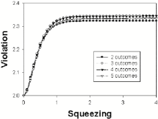
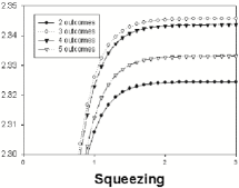
Figure 1: (a) Violation of local realistic bound 2 with complex observable for a two-mode squeezed state. Re-scaled figure (b) clearly shows the difference between the strength of violation for the different numbers of measurement outcome.

Conclusions - In many of the $d$-outcome nonlocality test, the observable can be non-Hermitian giving a complex number as a measurement outcome. It is not obvious how to construct an experiment for such a measurement. We have proposed, for the first time, an efficient and feasible scheme to test Bell’s inequality for an arbitrary number of measurement outcomes on CV systems. The nonlocal correlation functions directly corresponds to quasiprobability functions with complex ordering parameter in phase space. This relation makes the experimental realization for the $d$-outcome nonlocality test feasible. We have shown that entangled CV systems can violate this Bell inequality beyond the limits obtained in the tests of standard Bell’s inequalities for dichotomic observables.

We acknowledge support of the UK EPSRC, Austrian Science Foundation (FWF) Project SFB 1506, European Commission (RAMBOQ), KRF (2003-070-C00024) and the British Council in Austria.

References

- (1) S.L. Braunstein and P. van Loock, Rev. Mod. Phys. 77, 513 (2005).
- (2) Č. Brukner et al., Phys. Rev. A68, 062105 (2003).
- (3) A. Einstein, B. Podolsky, and N. Rosen, Phys. Rev. 47, 777 (1935).
- (4) J. S. Bell, Speakable and Unspeakable in Quantum Mechanics (Cambridge University Press, Cambridge, 1987).
- (5) K. Banaszek and K. Wodkiewicz, Phys. Rev. Lett. 82, 2009 (1999).
- (6) Z.-B. Chen et al., Phys. Rev. Lett. 88, 040406 (2002).
- (7) D. Collins et al., Phys. Rev. Lett. 88, 040404 (2002).
- (8) B.-G. Englert, N. Sterpi and H. Walther, Opt. Commun. 100, 526 (1993); L. G. Lutterbach and L. Davidovich, Phys. Rev. Lett. 78, 2547 (1997).
- (9) P. Bertet et al., Phys. Rev. Lett. 89, 200402 (2002).
- (10) W. Son, J. Lee and M. S. Kim, Phys. Rev. Lett. 96, 060406 (2006).
- (11) Each correlation term in Eq. (4) can be written as with . Evaluating one of functions, for example , we have . Similarly, one can find and and with the given functions of , it is possible to check the equivalence of our Bell function and the CGLMP one.
- (12) L. Masanes, Quantum Inf and Comp 3, 345 (2002).
- (13) K. E. Cahill and R. J. Glauber, Phys. Rev. 177, 1857 (1969); ibid, 1882 (1969).
- (14) K. Vogel and H. Risken, Phys. Rev. A40, R2847 (1989); M. G. Raymer, D. F. McAlister and U. Leonhardt, Phys. Rev. A54, R2397 (1996).
- (15) F. de Melo et al., Phys. Rev. A73, 030303 (R) (2006).