Pulsed squeezed light: simultaneous squeezing of multiple modes

Abstract

We analyze the spectral properties of squeezed light produced by means of pulsed, single-pass degenerate parametric down-conversion. The multimode output of this process can be decomposed into characteristic modes undergoing independent squeezing evolution akin to the Schmidt decomposition of the biphoton spectrum. The main features of this decomposition can be understood using a simple analytical model developed in the perturbative regime. In the strong pumping regime, for which the perturbative approach is not valid, we present a numerical analysis, specializing to the case of one-dimensional propagation in a beta-barium borate waveguide. Characterization of the squeezing modes provides us with an insight necessary for optimizing homodyne detection of squeezing. For a weak parametric process, efficient squeezing is found in a broad range of local oscillator modes, whereas the intense generation regime places much more stringent conditions on the local oscillator. We point out that without meeting these conditions, the detected squeezing can actually diminish with the increasing pumping strength, and we expose physical reasons behind this inefficiency.

I Introduction

Squeezed states of the radiation field are those in which the field fluctuations in one of the quadratures are reduced below the vacuum noise level. They were among the first nonclassical states of light generated experimentally Slusher85 ; Wu86 in the 1980s, and were considered promising as a way of overcoming the shot-noise precision restrictions in optical measurements Grangier87 and enhancing the capacity of communication channels YuenShapiro80 . Nowadays, the interest to generate squeezed light is mainly due to its applicability in quantum information and communication. In this context it is viewed primarily as a means of generating quadrature entanglement Ou92 , a valuable resource that can be applied, for example, for quantum teleportation Furusawa98 , computation LLoyd99 , cryptography Ralph00 and manipulation of atomic quantum states Kuzmich00 . There has been also a theoretical effort towards developing protocols for the continuous-variable error correction Braunstein982 ; Lloyd98 and entanglement purification Duan00 . Furthermore, operations that enable entanglement distillation in the continuous-variable domain have been described BrowEisePRA03 .

The present paper concentrates on one experimental method for producing optical squeezing, namely an optical parametric amplifier (OPA), implementing degenerate parametric down-conversion in a single-pass, pulsed configuration. A strong pump pulse propagating through a nonlinear crystal generates pairs of down-converted photons. The idealized experimental arrangement would be such that the photons in each generated pair are completely indistinguishable and contribute to the same spatio-temporal mode of the generated field. A combination of a high pump pulse energy and high optical nonlinearity leads to multiple pair creation events, which can be described in the Heisenberg picture as a linear transformation between the field operators at the input $\hat{a}_{in}$ and the output $\hat{a}_{out}$ of the amplifier:

$$\hat{a}_{out}=\hat{a}_{in}\,\cosh\zeta+\hat{a}^{\dagger}_{in}\,\sinh\zeta.$$ (1)

When the initial state of the field is vacuum, the above equation defines a squeezed state with the degree of squeezing $\zeta$, corresponding to the mean square quadrature noise scaling factor equal to $e^{-2\zeta}$. A crucial assumption underlying Eq. (1), frequently used in theoretical works, is that all the down-converted photons are emitted to a single mode described by the annihilation operator $\hat{a}_{out}$. However, this does not correspond to a realistic experimental situation.

In an experiment, pulsed squeezed light was realized for the first time by Slusher et al. laporta and has since been reproduced and improved by a number of researchers Kumar ; Kim ; Anderson ; Daly ; Smithey . In all these experiments, a pulsed laser is first frequency doubled and then undergoes parametric down-conversion in a spatially- and spectrally-degenerate type I configuration. The generated optical state is then characterized by means of homodyne detection. In contrast to the continuous-wave regime, the pulsed squeezed mode does not associate with a sideband of the carrier wave, but is localized within the temporal frame of the pump laser pulse Sasaki05 . This appealing feature is however compromised by a complex spectral structure of the generated photon pairs. In single-pass down-conversion, biphotons are emitted not necessarily into a particular mode, but into a wide range of modes restricted only by the energy-conservation and phase-matching conditions. The usual absence of a dominant spatio-temporal mode can lead to difficulties when we attempt to observe quantum interference of the generated squeezed vacuum with other classical or nonclassical optical states. The negative effects range from efficiency reduction in homodyne detection to extra dark counts in single photon measurements.

The present paper is dedicated to studying the spectral mode of the pulsed squeezed state. A particular question we aim to answer is the following: can we define a particular mode in which high-efficiency squeezing is achieved? Are there methods to engineer this mode and what are the most efficient ways to access it in homodyne measurements? The arguments given in the previous paragraph may lead one to believe that there is no mode in which high-efficiency squeezing is present. Surprisingly, we demonstrate just the opposite: we find modes in which pure squeezed states are generated, and also a whole continuum of their phase-locked superpositions turns out to become efficiently squeezed. In fact, good squeezing is present in a broad, continuous range of pulsed modes that are temporally synchronized with the pump.

The basic theoretical tool in our analysis will be the Bloch-Messiah reduction of an arbitrary Bogoliubov transformation of bosonic field operators BraunsteinSq . This procedure will allow us to identify a set of independent squeezing modes whose evolution takes a simple form analogous to Eq. (1). Such a decomposition results directly from the preservation of the commutation relations between the field operators in course of the parametric evolution. This fact allows us to apply the numerical technique of singular-value decomposition to integral kernels describing the transformation of the field operators, which provides effective means to analyze a realistic parametric amplifier. The decomposition into independent squeezers has been given previously by Bennik and Boyd Bennink , who deduced it using intricate operator algebraic methods Ma1990 .

As a physical example, we analyse one-dimensional propagation in a beta-barium borate (BBO) crystal serving as a model of a waveguide amplifier. The nonlinearity of a BBO crystal has an instantaneous character BoydNLO , as this medium is transparent from infrared to ultraviolet and we find that the downconversion spectrum is limited by the dispersion across the signal frequencies. This differs from the example studied in Ref. Bennink which assumed noninstantaneous second-order nonlinearity leading to limited downconversion spectrum, while the dispersion within the bandwidth of down-converted frequencies was neglected. Also, we discuss in detail the perturbative regime of weak conversion efficiency which provides intuitive insights into the structure of squeezing building on previous results obtained for spectral two-photon wave functions Keller ; GricePRA97 ; Law00 . We also show that the characteristic squeezing modes of a parametric amplifier provide a general answer to the question of optimizing the local oscillator shape in homodyne measurements MJWernerPRA95 ; ShapiroJOSAB97 .

This paper is organized as follows. In Sec. II we give theoretical foundations of the decomposition used to analyze the structure of squeezing in the parametric process. Then in Sec. III we discuss the weak pumping regime with a low pair creation probability per pulse and show that the squeezing modes are defined primarily by the material dispersion coefficients. The general case of strong pump fields which needs to be solved numerically is addressed in Sec. IV. The consequences of the multimode character of the output field for homodyne detection are studied in detail in Sec. V. Finally, Sec. VI concludes the paper.

II General model of an OPA

The subject of our analysis is one-dimensional propagation of an optical field through a nonlinear medium in which three-wave mixing takes place. For simplicity and specificity, we will focus here on the one-dimensional case that can be realized in non-linear waveguides NonlinearWaveguides , which recently have become available commercially. The one-dimensional case nevertheless includes all the complexities of multimode propagation in the spectral degree of freedom, and the generalization of the formalism introduced here to the full three-dimensional case is straightforward.

If the pump field is strong enough to neglect its depletion as well as fluctuations, the propagation equations in the Heisenberg picture become linear in the signal field. Following the standard nonlinear optics description of the evolution of the fields with respect to the distance covered rather than time, we shall adopt the modal decomposition of the electric field operator in the form

$$\hat{E}(z,t)=i\int\frac{d\omega}{2\pi}\sqrt{\frac{\hbar\omega}{2\epsilon_{0}\sqrt{n(\omega)}}}\,e^{-i\omega t}\hat{a}(\omega;z)+\text{H.c.}$$ (2)

where $\epsilon_{0}$ is the permittivity of the vacuum, $n(\omega)$ is the refractive index of the medium at a given frequency and polarization direction, $\hat{a}(\omega;z)$ is the annihilation operator of a monochromatic mode at a given propagation stage indicated by $z$. We have neglected the dependence of the field on transverse coordinates, as we concentrate here on the one-dimensional case of a waveguide. The quantization of the classical propagation equations of the three-wave mixing problem KlasycznaReferencja is done by a formal substitution of classical amplitudes by field operators. This yields a first-order differential equation for annihilation operators $\hat{a}(\omega;z)$ of the form:

$$\frac{\partial\hat{a}(\omega;z)}{\partial z}=ik(\omega)\hat{a}(\omega;z)$$

$$+\frac{1}{L_{\mathrm{NL}}E_{0}}\int d\omega^{\prime}\,e^{ik_{p}(\omega^{\prime}+\omega)z}E_{p}(\omega^{\prime}+\omega)\hat{a}^{\dagger}(\omega^{\prime};z)$$

where the first term on the right-hand side represents the free propagation of the field in the medium, while the second one represents nonlinear interaction. In the above expression, $E_{p}(\omega)$ is the spectral amplitude of the pump field at the point $z=0$, which is chosen half-way through the waveguide of a total length $L$, $\omega_{p}$ is the central frequency of the pump spectrum, $k(\omega)$ and $k_{p}(\omega)$ are the signal and the pump field wavevectors, respectively, and we rescaled the spectral amplitude of the pump field by introducing $E_{0}=\int d\omega E_{p}(\omega)$. For all calculations in this paper, $E_{p}(\omega)$ is assumed real and positive, i.e. the pump pulse is prepared so that in the middle of the waveguide it is not chirped.

With this choice, the multiplicative constant $L_{\mathrm{NL}}$ is the characteristic length of the nonlinear interaction defined as

$$\frac{1}{L_{\mathrm{NL}}}=\frac{\omega_{p}^{2}\,d_{\mathrm{eff}}E_{0}}{8c^{2}k(\omega_{p}/2)},$$ (4)

where $d_{\mathrm{eff}}$ is the effective nonlinearity coefficient for the given polarization directions in the medium and $\omega_{p}/2$ is assumed to be the central frequency of the signal field. When introducing $L_{\mathrm{NL}}$, we assumed that the frequency dependence of $d_{\mathrm{eff}}$ combined with the normalization factors in the modal decomposition given in Eq. (2) yields a constant whose changes over the bandwidth of the signal field can be neglected. The physical interpretation of $L_{\mathrm{NL}}$ is that when the signal field is restricted to a single frequency mode and no phase mismatch with the pump field is present, $L_{\mathrm{NL}}$ is the length over which the minimum and the maximum RMS quadrature noise scales by $e$. This corresponds to the single-mode degree of squeezing introduced in Eq. (1) equal to $\zeta=L/L_{\mathrm{NL}}$. Let us note that $1/L_{\mathrm{NL}}$ is proportional to the pump pulse amplitude, which we will further refer to as the pumping strength.

It is instructive to recast Eq. (LABEL:aprop) into a standard form which allows us to compare different quantum mechanical pictures of the evolution of a system. Explicitly, the development of the field operators described by Eq. (LABEL:aprop) can be written as:

$$\frac{\partial\hat{a}(\omega;z)}{\partial z}=i[\hat{H},\hat{a}(\omega;z)]$$ (5)

where the operator $\hat{H}$, formally equivalent to the Hamiltonian governing the evolution of the system, is given by a sum of two terms $\hat{H}=\hat{H}_{0}+\hat{V}(z)$. The first term generates linear propagation:

$$\hat{H}_{0}=-\int d\omega\,k(\omega)\hat{a}^{\dagger}(\omega)\hat{a}(\omega)$$ (6)

while the second term is responsible for the three-wave mixing process:

$$\hat{V}(z)=\frac{1}{2L_{\mathrm{NL}}E_{0}}\int d\omega d\omega^{\prime}$$

$$\times[ie^{ik_{p}(\omega^{\prime}+\omega)z}E_{p}(\omega^{\prime}+\omega)\hat{a}^{\dagger}(\omega)\hat{a}^{\dagger}(\omega^{\prime})+{\rm H.c.}].$$

The evolution of the quantum state of light while propagating through the crystal can in principle be evaluated in the interaction picture by integrating over $z$ the term $\hat{V}(z)$. This is however highly complicated because the Hamiltonian (II) is position-dependent and generally does not commute with itself at different values of $z$. Consequently, the evolution operator needs to be appropriately ordered in its expansion in $\hat{V}(z)$. As we discuss in the next section and in the Appendix, this ordering can sometimes be neglected and decomposition into squeezing eigenmodes can be performed efficiently using the interaction picture. The general case is however best described using the Heisenberg picture approach.

As the propagation equation given in Eq. (LABEL:aprop) is linear in the field operators, for any given waveguide length $L$ we can find Green functions $C(\omega,\omega^{\prime})$ and $S(\omega,\omega^{\prime})$ that transform the input field operators $a^{in}(\omega)\equiv a(\omega;-L/2)$ into output field operators $a^{out}(\omega)\equiv a(\omega;L/2)$ according to:

$$\hat{a}^{out}(\omega)=\int d\omega^{\prime}[C(\omega,\omega^{\prime})\,\hat{a}^{in}(\omega^{\prime})+S(\omega,\omega^{\prime})\,\hat{a}^{in\,\dagger}(\omega^{\prime})].$$ (8)

The above Bogoliubov transformation can be brought into a canonical form by applying the Bloch-Messiah reduction BraunsteinSq which we will now briefly review. The relevant mathematical tool is the singular value decomposition applied to the Green functions $C(\omega,\omega^{\prime})$ and $S(\omega,\omega^{\prime})$. Because the output annihilation operators must satisfy canonical commutation relations, the functions $C(\omega,\omega^{\prime})$ and $S(\omega,\omega^{\prime})$ are connected through a number of relations. In particular, the singular value decompositions of both $C(\omega,\omega^{\prime})$ and $S(\omega,\omega^{\prime})$ can be represented using a shared set of parameters and functions. The explicit formulas have the following form:

$$C(\omega,\omega^{\prime}) = \sum_{n=0}^{\infty}\psi^{*}_{n}(\omega)\,\cosh\zeta_{n}\,\phi_{n}(\omega^{\prime})$$

$$S(\omega,\omega^{\prime}) = \sum_{n=0}^{\infty}\psi^{*}_{n}(\omega)\,\sinh\zeta_{n}\,\phi^{*}_{n}(\omega^{\prime})$$ (9)

where $\phi_{n}(\omega)$ and $\psi_{n}(\omega)$ are two orthonormal bases and $\zeta_{n}$ are real nonnegative parameters. The existence of such a joint decomposition allows us to introduce two sets of operators for input and output modes, defined according to

$$\hat{b}^{in}_{n} = \int d\omega\,\phi_{n}(\omega)\hat{a}^{in}(\omega)$$

$$\hat{b}^{out}_{n} = \int d\omega\,\psi_{n}(\omega)\hat{a}^{out}(\omega)\,,$$ (10)

where $\hat{b}^{in}_{n}$ and $\hat{b}^{out}_{n}$ are the corresponding annihilation operators which satisfy the standard commutation relations. Consequently, we can recast the general transformation given in Eq. (8) into a simple form of single-mode squeezing transformations acting in parallel on orthogonal modes:

$$\hat{b}^{out}_{n}=\cosh\zeta_{n}\,\hat{b}^{in}_{n}+\sinh\zeta_{n}\,\hat{b}^{in\,\dagger}_{n},$$ (11)

bringing us back to the elementary expression given in Eq. (1).

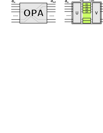
Figure 1: Pictorial representation of the Bloch-Messiah theorem. Any Bogoliubov transformation of input modes $\hat{a}^{in}_{n}$ into output modes $\hat{a}^{out}_{n}$ can be decomposed into a passive transformation $U={\phi_{n}}$ from modes $\hat{a}^{in}_{n}$ into $\hat{b}^{in}_{n}$ followed by independent squeezers with gains $G_{n}$ and another passive transformation $V={\psi^{*}_{n}}$ from $\hat{b}^{out}_{n}$ into $\hat{a}^{out}_{n}$.

Since any linear transformation of the form given in Eq. (8) can be decomposed into orthogonal modes which undergo independent evolution, the above procedure, summarized graphically in Fig. 1, can be applied to any combination of processes such as linear optics, optical amplification, and Kerr squeezing. Were we able to separate modes $\psi_{n}(\omega)$ spatially, we could turn a realistic parametric amplifier into a generator of multiple pure squeezed states Opatrny .

Let us note that the procedure of singular value decomposition applied above is formally equivalent to Schmidt decomposition of a quantum state of a bipartite system. In the next section and in the Appendix, this equivalence will allow us to connect the general decomposition to previous treatments of parametric down-conversion in the perturbative regime.

One interesting feature of the squeezing eigenmodes is that for real $E_{p}$ (i.e. the pump pulse in the middle of the waveguide is not chirped or its chirp is insignificant),

$$\psi_{n}(\omega)=\phi^{*}_{n}(\omega).$$ (12)

This is proven by noticing the symmetry of Eq. (LABEL:aprop) with respect to the point $z=0$. Indeed, it can be rewritten as follows:

$$\frac{\partial\hat{a}(\omega;z)}{\partial(-z)}=-ik(\omega)\hat{a}(\omega;z)$$

$$-\frac{1}{L_{\mathrm{NL}}E_{0}}\int d\omega^{\prime}\,e^{-ik_{p}(\omega^{\prime}+\omega)(-z)}E_{p}(\omega^{\prime}+\omega)\hat{a}^{\dagger}(\omega^{\prime};z),$$

which can be formally interpreted as reverse propagation of the quantum field from $-z=-L/2$ to $-z=L/2$. Integrating Eq. (LABEL:apropx) between these two points we write, by analogy with Eq. (8):

$$\hat{a}^{in}(\omega)=\int d\omega^{\prime}[\tilde{C}(\omega,\omega^{\prime})\,\hat{a}^{out}(\omega)+\tilde{S}(\omega,\omega^{\prime})\,\hat{a}^{\dagger\,out}(\omega)],$$ (14)

where the superscripts $in$ and $out$ refer, as previously defined, to the points $z=-L/2$ and $z=L/2$, respectively. Comparing Eqs. (LABEL:aprop) and (LABEL:apropx), we establish a simple relation between the Green functions of direct and reverse propagation: $\tilde{C}(\omega,\omega^{\prime})=C^{*}(\omega,\omega^{\prime})$ and $\tilde{S}(\omega,\omega^{\prime})=-S^{*}(\omega,\omega^{\prime})$. Decomposing the latter according to Eq. (9)

$$\tilde{C}(\omega,\omega^{\prime}) = \sum_{n=0}^{\infty}\psi_{n}(\omega)\,\cosh\zeta_{n}\,\phi^{*}_{n}(\omega^{\prime})$$

$$\tilde{S}(\omega,\omega^{\prime}) = \sum_{n=0}^{\infty}\psi_{n}(\omega)\,\sinh(-\zeta_{n})\,\phi_{n}(\omega^{\prime}),$$ (15)

we find, in addition to (10), another set of propagation eigenmodes

$$\hat{\tilde{b}}^{in}_{n} = \int d\omega\,\psi^{*}_{n}(\omega)\hat{a}^{in}(\omega)$$

$$\hat{\tilde{b}}^{out}_{n} = \int d\omega\,\phi^{*}_{n}(\omega)\hat{a}^{out}(\omega)$$ (16)

with characteristic squeezing parameters $\zeta_{n}$. Assuming that all $\zeta_{n}$ are unequal (which is typically the case as we show below), the Bloch-Messiah decomposition is unique, and we conclude that $\hat{\tilde{b}}^{in}_{n}=\hat{b}^{in}_{n}$ and $\hat{\tilde{b}}^{out}_{n}=\hat{b}^{out}_{n}$, which leads to Eq. (12). In the time domain, this identity corresponds to the output modes being the time reversal of the input.

Finally, let us point out that the decomposition given in Eq. (9) has important implications when considering a parametric amplifier seeded with a coherent pulse. The reason for seeding the parametric amplifier is to impose a mode in which the majority of the output photons is generated, thus overwhelming emission to other modes whose contents can be neglected as an unimportant background Smithey92 . Eq. (11) indicates that the output of the parametric amplifier will contain a pure squeezed coherent state in a single mode if the seeding coherent state occupies one of the characteristic input modes $\phi_{n}(\omega)$. If the seeding pulse is in superpositon of many modes $\phi_{n}(\omega)$, under the action of the parametric amplifier it will generate multiple squeezed coherent modes, in principle each one of different intensity and squeezing parameter. The decomposition in Eq. (9) provides one with characteristic pulse profiles $\phi_{n}(\omega)$ which are optimal for seeding the amplifier.

III Single pair generation regime

In a general case, the equations of motion for the field operators specified by Eq. (LABEL:aprop) can be solved only by numerical means. Before we resort to numerical methods, we will discuss in this section an approximate solution to the problem in the weak conversion limit, when only the first order of the perturbation theory is relevant. This is indeed the case if the nonlinear interaction length $L_{\mathrm{NL}}$ is much greater that the crystal length $L$, thus keeping the squeezing weak. This approach will give us intuitive insights into the structure of the output field, and will help us to identify parameters relevant to its characterization in the arbitrary case.

The first order approximation to Eq. (8) can be obtained most easily by substituting

$$\hat{a}(\omega;z)=\exp(ik(\omega)z)\,\hat{a}_{I}(\omega;z)$$ (17)

into Eq. (LABEL:aprop), then integrating it over $z$ and retaining terms up to first order in $L/L_{\mathrm{NL}}$. This procedure yields an expression for $\hat{a}(\omega;L)$. Using this result we find the approximate Green functions in the form:

$$C(\omega,\omega^{\prime}) = \delta(\omega-\omega^{\prime})e^{ik(\omega)L}$$ (18)

$$S(\omega,\omega^{\prime}) = \frac{LE_{p}(\omega+\omega^{\prime})}{L_{\mathrm{NL}}E_{0}}\,e^{i[k(\omega)-k(\omega^{\prime})]L/2}\,\mathrm{sinc}\frac{L\Delta k}{2}$$

where

$$\Delta k=k_{p}(\omega+\omega^{\prime})-k(\omega)-k(\omega^{\prime})$$ (20)

is the phase mismatch between the pump and the pair of down-converted photons.

In most cases it is sufficient to expand $\Delta k$ up to the second order in deviations from the respective central frequencies. Then the approximate expression for the phase mismatch takes the form:

$$\Delta k \simeq (\beta_{1,p}-\beta_{1})(\omega+\omega^{\prime}-\omega_{p})$$ (21)

$$-\frac{1}{2}\beta_{2}\left((\omega-\omega_{p}/2)^{2}+(\omega^{\prime}-\omega_{p}/2)^{2}\right)$$

$$+\frac{1}{2}\beta_{2,p}(\omega+\omega^{\prime}-\omega_{p})^{2},$$

where

$$\beta_{n} =\frac{d^{n}k(\omega)}{d\omega^{n}}\Big{|}_{\omega=\omega_{p}/2}$$ (22a)

$$\beta_{n,p} =\frac{d^{n}k_{p}(\omega)}{d\omega^{n}}\Big{|}_{\omega=\omega_{p}}$$ (22b)

are dispersion coefficients for the pump and the signal fields. The coefficients relevant to our analysis are: the difference of inverse group velocities $\beta_{1,p}-\beta_{1}$ and the group velocity dispersion coefficients $\beta_{2}$ and $\beta_{2,p}$. The phase term $e^{i[k(\omega)-k(\omega^{\prime})]L/2}$ in Eq. (LABEL:S'1st) arises form the free propagation of the squeezed field in the waveguide.

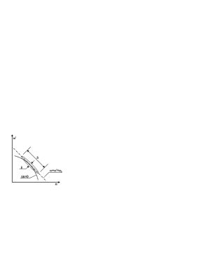
Figure 2: Gaussian approximation of the Green function $S(\omega,\omega^{\prime})$, given in Eq. (LABEL:S'1st) by a product of the pump spectral amplitude and the phasematching function. The first factor is nonzero on a wide strip centered around the $\omega_{s}+\omega_{i}=\omega_{p}$ line. The second factor is nonzero on a strip lying along the $\Delta k=0$ line, which is approximately parabolic and tangent to the line $\omega_{s}+\omega_{i}=\omega_{p}$ at the point $(\omega_{p}/2,\omega_{p}/2)$. Thus the product $S(\omega,\omega^{\prime})$ is nonzero on a strip ariound the $\omega_{s}+\omega_{i}=\omega_{p}$ line and extending to points where the phasematching function goes off the pump spectral amplitude.

Physically, performing the expansion up to the first order in $L/L_{\mathrm{NL}}$ means considering only generation of single photon pairs. The spectral properties of single photon pairs generated by ultrashort pulses have been extensively studied in the context of quantum indistinguishability in two-photon interference experiments GricePRA97 ; Keller ; Perina ; Law00 . The basic entity in those studies is the two-photon wave function $\Psi(\omega,\omega^{\prime})=\langle 1_{\omega},\,1_{\omega^{\prime}}|\Psi^{out}\rangle$ describing the probability amplitude of generating a pair of photons with frequencies $\omega$ and $\omega^{\prime}$. In the Appendix, we relate this wave function to the Green function $S(\omega,\omega^{\prime})$ through a simple formula:

$$\Psi(\omega,\omega^{\prime})=S(\omega,\omega^{\prime})e^{ik(\omega^{\prime})L}.$$ (23)

In other words, the eigenmodes of pulsed squeezing are closely related to the eigenmodes of the Schmidt decomposition of a biphoton spectrum originally found by Law et al. Law00 .

Identity (23) suggests a Gaussian approximation similar to that applied in the analysis of the two-photon wave function GricePRA01 , which will yield a singular value decomposition in a closed analytical form. For this purpose, let us assume that the quadratic form of the Gaussian which approximates Eq. (LABEL:S'1st) has the principal axes given by $\omega-\omega^{\prime}=0$ and $\omega+\omega^{\prime}=\omega_{p}$, and seek an expression of the form:

$$S_{G}(\omega,\omega^{\prime})= \sqrt{\frac{2N}{\pi\delta\Delta}}\,e^{i[k(\omega)-k(\omega^{\prime})]L/2}$$

$$\times\exp\left[-\frac{(\omega+\omega^{\prime}-\omega_{p})^{2}}{2\delta^{2}}-\frac{(\omega-\omega^{\prime})^{2}}{2\Delta^{2}}\right]$$ (24)

In order to find the unknown coefficients in the above formula, let us take a Gaussian pump pulse of duration $\tau_{p}$:

$$E_{p}(\omega)\propto\exp\left[-\frac{\tau_{p}^{2}}{2}(\omega-\omega_{p})^{2}\right].$$ (25)

We insert the expansion given in Eq. (21) into Eq. (LABEL:S'1st), apply the following approximations to the sinc function along the axes $\omega-\omega^{\prime}=0$ and $\omega+\omega^{\prime}=\omega_{p}$:

$$\mathrm{sinc}\,x\approx e^{-x^{2}/5},\;\mathrm{sinc}(x^{2})\approx e^{-x^{2}/3},$$ (26)

and compare Eq. (LABEL:S'1st) after all these approximations with Eq. (24) along the principal axes. This yields:

$$\frac{1}{\delta^{2}} \approx \tau_{p}^{2}+\frac{L^{2}}{10}(\beta_{1}-\beta_{1,p})^{2}$$ (27a)

$$\frac{1}{\Delta^{2}} \approx \frac{1}{12}L\beta_{2}$$ (27b)

$$N = \int|S_{G}(\omega,\omega^{\prime})|^{2}d\omega d\omega^{\prime}=\frac{L^{2}}{4L_{\mathrm{NL}}^{2}}\tau_{p}^{2}\delta\Delta\quad$$ (27c)

The meaning of these parameters is depicted in Fig. 2. Typically Shapiro , $\delta\ll\Delta$ and consequently the bandwidth of the downconverted light is approximately proportional to $\Delta$. In the particular case of type I phasematching this bandwidth is limited mostly by the group velocity dispersion $\beta_{2}$ at signal frequencies. Note that, in contrast, the difference between the group velocities at the pump and the signal frequencies $\beta_{1}-\beta_{1,p}$ sets no limit on the downconversion spectrum. The second relevant frequency scale is set by the parameter $\delta$ which characterizes the width of the spectral correlation between photons in pair. This width is limited by the pump pulse bandwidth and the group velocity difference $\beta_{1}-\beta_{1,p}$. Also, let us note that the Green function $S(\omega,\omega^{\prime})$ is not normalized, and its contribution is implicitly assumed to be small, of the order $L/L_{\mathrm{NL}}$, as compared to that of $C(\omega,\omega^{\prime})$. The normalization constant $N$ of $S_{G}(\omega,\omega^{\prime})$ given in Eq. (27c) is equal to the total number of photons per pulse emitted by the downconversion source.

Since in general $\Delta$ and $\delta$ are different, one cannot simply factorize $S(\omega,\omega^{\prime})$ and define a single mode into which photon pairs are emitted. If the signal and idler photons were nondegenerate, one would call such a spectrum entangled; this definition is however inapplicable to the present situation because the two fields cannot be separated using another degree of freedom. With the Gaussian approximation in hand, let us now employ the summation formula used previously to find the Schmidt decomposition of a bipartite Gaussian state ActaPhysicaSlovaca ; GricePRA01 , which can be applied directly to the Green function (24) in order to find its singular value decomposition. Recasting the decomposition according to the general expression specified in Eq. (9), we obtain that the squeezing parameters $\zeta_{n}$ form a geometric sequence given by:

$$\zeta_{n}\approx\sinh\zeta_{n}=\frac{\sqrt{N}}{\cosh r}\tanh^{n}r$$ (28)

with the parameter $r=\ln(\Delta/\delta)/2$, while the corresponding eigenmodes are described by the Hermite functions:

$$e^{-ik(\omega)L/2}\psi_{n}(\omega) = e^{ik(\omega)L/2}\phi_{n}(\omega)$$

$$= \frac{H_{n}(\omega\tau_{s})}{\sqrt{2^{n}n!}}\sqrt{\frac{\tau_{s}}{\sqrt{\pi}}}e^{-\tau_{s}^{2}(\omega-\omega_{p}/2)^{2}/2},$$

with characteristic spectral width of all squeezing modes being proportional to the inverse geometric mean of the two spectral widths $\delta$ and $\Delta$:

$$\tau_{s}=\sqrt{\frac{2}{\delta\Delta}}.$$ (30)

These expressions for the eigenmodes and the squeezing parameters will serve as a reference when analyzing numerical results in the nonperturbative regime presented in the next section.

As expected, $\psi_{n}(\omega)=\phi^{*}_{n}(\omega)$, and the modes’ spectral phases can be attributed to the linear dispersive propagation through the BBO crystal. The nonzero phase profiles are difficult to handle experimentally. One might think they can be made negligible by choosing a sufficiently long pump pulse so its dispersion can be neglected. This is however not the case because the eigenmodes’ characteristic spectral width $1/\tau_{s}$ is determined not only by $\delta$, but also by $\Delta$. The magnitude $\Delta$ is, in turn, determined by the properties of the crystal rather than the pump pulse and is usually large.

The fact that the phase profiles of squeezing eigenmodes depend on the crystal length has an interesting consequence. Suppose we prepare a particular state of light in a squeezing eigenmode $b_{n}^{in}(L)$ of a crystal of length $L$ and insert it into the crystal. After propagation through the entire crystal, this state will undergo squeezing and leave the crystal in the mode $b_{n}^{out}(L)$. Now we ask, what will be the state of light at the point $z=0$ half way through the crystal? Propagation of light to this point is equivalent to that through a crystal of length $L/2$. The mode $b_{n}^{in}(L)$ is however not an eigenmode associated with this crystal; therefore, the state of light at $z=0$ cannot be defined in any pure mode, but only as an entangled state of many modes. We see that while light enters and leaves the crystal in a pure optical mode and state, inside the crystal all input modes temporarily become entangled with each other.

IV Intense generation regime

In this section, we discuss numerical solutions to the propagation equation (LABEL:aprop) in a general, not necessarily perturbative regime. As a concrete example, we will consider type-I interaction in a BBO crystal. We assume that a waveguide is formed in a direction of perfect phase matching for an interaction of a 400 nm pump wave with 800 nm signal waves (corresponding to the angle between the waveguide axis and the optical axis $\theta=29.2^{o}$). For this system, we have solved numerically Eq. (LABEL:aprop) with $k(\omega)$ and $k_{p}(\omega)$ approximated by values for a bulk BBO crystal, and a Gaussian pump field given by Eq. (25). Let us stress that in the calculations presented below we use neither the crude Gaussian approximation of the sinc phasematching function, nor are we limited to the first order accuracy in $L/L_{\mathrm{NL}}$. Nevertheless, the simple model developed in the preceding section will guide us through general solutions.

As the propagation equation is linear in the strong undepleted pump approximation, Eq. (LABEL:aprop) is identical to the classical equation of motion for a pulse propagating through a waveguide, with the annihilation operators $\hat{a}(\omega;z)$ replaced by the spectral amplitudes of the electric field at respective signal frequencies $\alpha(\omega;z)$ KlasycznaReferencja . Thus we can compute numerically the matrix approximations to the Green functions $C(\omega,\omega^{\prime})$ and $S(\omega,\omega^{\prime})$ using the well-established in classical nonlinear optics split-step method for solving partial differential equations. The approximations are obtained by solving the propagation equation for a complete set of $\delta$-function shaped initial conditions where the classical signal field $\alpha(\omega;z=-L/2)$ is taken to be equal to zero everywhere on the computational grid in the frequency domain, except for a single point of the grid at which it assumes $1$ or $i$. When the distinguished point corresponds to the frequency $\omega^{\prime}$, solving the propagation equation with such initial conditions yields single columns of the discretized Green functions $C(\omega,\omega^{\prime})$ and $S(\omega,\omega^{\prime})$. After calculating all the columns of the Green functions, we computed the singular-value decompositions defined in Eq. (9) which gives the desired Bloch-Messiah reduction.

We assessed whether the computational grid was fine enough to support all the modes with nonunit gain by checking that the squeezing parameters for high-order modes approach zero. Additional tests of computational accuracy consisted in verifying that the singular values of $C(\omega,\omega^{\prime})$ and $S(\omega,\omega^{\prime})$ are pairwise sinh and cosh functions of the same real number, as stated in Eq. (9) and that the calculated modes uphold the relation (12). Although many modes are not included in our numerical calculation, we argue that their squeezing is negligible, thus the actual choice of the mode functions $\phi_{n}(\omega)$ and $\psi_{n}(\omega)$ representing them is unimportant.

Following the approach used in nonlinear optics, the calculations were performed in the reference frame of the down-converted light, moving with the group velocity $1/\beta_{1}$. This corresponds to substituting

$$\hat{a}(\omega;z)\rightarrow e^{i[\beta_{0}+\beta_{1}(\omega-\omega_{p}/2)]z}\,\hat{a}(\omega;z)$$ (31)

into the propagation equation given in Eq. (LABEL:aprop). The mode functions $\phi_{n}(\omega)$ and $\psi_{n}(\omega)$ will be given also in the moving reference frame. This reduces to stripping the mode functions from the linear phase in the expansion around $\omega_{p}/2$. Experimentally, the linear phase can be always corrected by adjusting the temporal delay of the down-conversion beam, whereas higher order phase terms lead to pulse distortions requiring dispersion management.

In our numerical calculations we used a Gaussian pump pulse of length $\tau_{p}=24$ fs (40 fs intensity FWHM) and the waveguide length $L=1$ mm. This corresponds to the inverse bandwidth of the downconversion light $\Delta^{-1}\simeq 4$ fs and the inverse of the spectral width of correlations between the two photon in a pair $\delta^{-1}\simeq 50$ fs. We will study how the features of the down-converted light depend on the nonlinear interaction length $L_{\mathrm{NL}}$.

We found that up to $L/L_{\mathrm{NL}}=15$ (which corresponds to over 100 dB maximal quadrature squeezing) the squeezing parameter of any squeezed mode is inversely proportional to nonlinear length with a specific proportionality constant. These values are depicted in Fig. 3. We note a substantial discrepancy with the Gaussian model from Sec. III, which predicts that the squeezing parameters should follow a geometric sequence (28), represented by a straight line in the semi-log scale plot in Fig. 3.

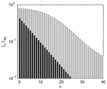
Figure 3: The rescaled squeezing parameters $L_{\mathrm{NL}}\zeta_{n}$ as a function of the mode number, verified numerically to be independent of $L_{\mathrm{NL}}$ for $L/L_{\mathrm{NL}}\leq 15$. Empty bars depict results of the numerical computation, while black bars represent predictions of the Gaussian approximation.

The Gaussian approximation turns out to be much more successful in predicting the shapes of the characteristic squeezing modes. Particularly in the weak pumping regime, the numerically calculated input and output modes $\phi_{n}(\omega)$ and $\psi_{n}(\omega)$ for low $n$ are almost identical to the Hermite-Gaussian functions predicted by Eq. (III), with only a slight asymmetry and more abrupt decay of their outermost wings (Fig. 4). For strong pumping, when the nonlinear interaction length $L_{\mathrm{NL}}$ becomes comparable or smaller than the crystal length $L$, the spectral intensity profiles begin to broaden and change in shape (Fig. 5) due to nonlinear modulation of the optical fields. Still, within the range of the interaction lengths studied here (i.e. $L/L_{\mathrm{NL}}\leq 15$), the Hermite-Gaussian approximation for the several most strongly squeezed modes works reasonably well. We expect this to be the case as long as the higher order terms in the phase mismatch expansion (21) are negligible. In the case of BBO, this condition is satisfied for $\tau_{p},\tau_{s}\gg 10$ fs.

In order to characterize the change in the mode widths, we fitted the numerically obtained spectral intensities $|\psi_{n}(\omega)|^{2}$ with the Gaussian-Hermite approximations Eq. (III) for each $L_{\mathrm{NL}}$ and $n$, treating the characteristic time $\tau_{s}$ as a free parameter. We found this parameter to deviate from the constant 20 fs value predicted by Eq. (30), and, as evidenced by Fig. 6, to depend on both the mode number and the pumping strength. In the weak pumping regime, $\tau_{s}\approx 15$ fs for $n=0$ and reduces by about 3% for each subsequent mode, and is independent from $L_{\mathrm{NL}}$. For stronger pumping ($L_{\mathrm{NL}}\gtrsim 1$), $\tau_{s}$ falls quickly with the increasing pumping strength.

As expected, we found the spectral phases of the input and the output modes to have opposite signs with virtually equal absolute values. For strong pumping, the phase profile also becomes flatter for shorter interaction lengths $L_{\mathrm{NL}}$, as illustrated in Fig. 5. Thus in the intense generation regime we can no longer attribute the spectral phase of the modes to linear dispersive propagation. All these effects mean that the features of multimode squeezing become more fragile compared to the single-pair generation case. Thus the exact modal characteristics need to be carefully taken into account when manipulating or detecting strongly squeezed light.

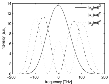
Figure 4: Spectral intensities $|\psi_{n}(\omega)|^{2}$ of the dominant three modes $n=0$ (solid line), $n=1$ (dashed line), and $n=2$ (dotted line) for $L_{\mathrm{NL}}=100$ mm.

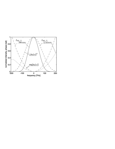
Figure 5: Spectral intensity and phase of the maximally squeezed mode $\psi_{0}(\omega)$ for $L_{\mathrm{NL}}=100$ mm (solid and dashed-dotted line respectively) and $L_{\mathrm{NL}}=1/15$ mm (dashed and dotted lines). For the case studied, the input modes are complex conjugate to output modes, $\phi_{0}(\omega)=\psi_{0}^{\ast}(\omega)$.

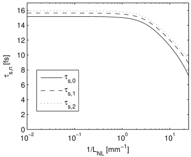
Figure 6: Duration of the dominant squeezed modes $\tau_{s,0}$ (solid line), $\tau_{s,1}$ (dashed line) and $\tau_{s,2}$ (dotted line) as a function of $1/L_{\mathrm{NL}}$, obtained by fitting Hermite-Gauss profiles from Eq. (III) to numerical results.

V Homodyne detection

Homodyne detection is a fundamental diagnostic and measurement technique in applications of squeezed states for quantum-enhanced metrology and continuous-variable quantum information processing. It is a difficult measurement because of the electronic noise, losses in the paths of the squeezed beams and nonideal mode matching between squeezed field and local oscillator which defines the measured quadrature. This section is devoted to a detailed study of the latter issue, and the modal decomposition of a parametric amplifier introduced in Sec. II provides a natural framework for its discussion.

We will consider an unseeded optical parametric amplifier followed by a balanced homodyne detector with the local oscillator (LO) pulse prepared in a certain shape characterized by the mode function $\psi_{\text{LO}}(\omega)$. The quantity of interest is the measured quadrature noise. The analysis is straightforward in the particular case when the local oscillator employed in the homodyne measurement is prepared in one of the characteristic modes $\psi_{\text{LO}}(\omega)=\psi_{n}(\omega)$. This choice of the LO means that we are “listening” only to one of the independently squeezed characteristic modes of the amplifier, whose evolution is given by Eq. (11). For vacuum input, this mode evolves into a squeezed vacuum state with the squeezing parameter equal to $\zeta_{n}$. Thus the detected mean square quadrature noise $\langle Q^{2}_{n,\theta}\rangle$ as a function of the LO phase $\theta$ is equal to scaling :

$$\langle Q^{2}_{n,\theta}\rangle=\frac{1}{4}(e^{2\zeta_{n}}\sin^{2}\theta+e^{-2\zeta_{n}}\cos^{2}\theta).$$ (32)

In particular, the product of the maximum $\langle Q_{+}^{2}\rangle=e^{2\zeta_{n}}/4$ and the minimum $\langle Q_{-}^{2}\rangle=e^{-2\zeta_{n}}/4$ quadrature noise will be the same as for the vacuum state $\langle Q_{+}^{2}\rangle\langle Q_{-}^{2}\rangle=1/16$ — the minimum value allowed by the Heisenberg uncertainty relation.

In the general case of an arbitrary LO pulse shape we can calculate the quadrature noise level by decomposing $\psi_{LO}(\omega)$ in the basis of the characteristic output modes of the amplifier:

$$\psi_{LO}(\omega)=\sum_{n=0}^{\infty}M_{n}e^{i\theta_{n}}\psi_{n}(\omega),$$ (33)

where $M_{n}$ and $\theta_{n}$ are real numbers and we have assumed that the spectral amplitude $\psi_{LO}(\omega)$ is normalized to unity. It is important that the quantum quadrature fluctuations of different characteristic modes are independent because the mutually uncorrelated modes $\hat{b}^{in}_{n}$ independently evolve into $\hat{b}^{out}_{n}$. Thus, using the local oscillator of the form (33), we measure a sum of noise contributions from the quadratures $\langle Q^{2}_{n,\theta_{n}}\rangle$ weighted with $M_{n}^{2}$:

$$\langle Q^{2}_{LO}\rangle=\sum_{n=0}^{\infty}\frac{M_{n}^{2}}{4}(e^{2\zeta_{n}}\sin^{2}\theta_{n}+e^{-2\zeta_{n}}\cos^{2}\theta_{n})$$ (34)

In general, the above expression combines contributions from both squeezed and antisqueezed quadratures. However, if all the phases $\theta_{n}$ are equal, we can always bring them to $0$ by introducing an additional phase delay in the LO arm. Then the minimum quadrature noise that can be observed is below the shot noise limit:

$$\langle Q^{2}_{-}\rangle=\sum_{n=0}^{\infty}\frac{M_{n}^{2}}{4}\exp(-2\zeta_{n})\leq\frac{1}{4}.$$ (35)

The condition of equal phases $\theta_{n}$ can be easily realized in the single pair generation regime, because all the output modes Eq. (III) bear the same spectral phase associated with the linear propagation in the waveguide. Thus for an unchirped local oscillator with an arbitrary intensity spectrum $I_{LO}(\omega)$ we can optimize the amount of detected squeezing by making its phase equal to the phase acquired by the squeezed field during propagation through a crystal of length $L/2$:

$$\psi_{LO}(\omega)=\sqrt{I_{LO}(\omega)}\,e^{ik(\omega)L/2}\,.$$ (36)

Let us note that if some of the squeezing parameters $\zeta_{n}$ are equal — for concreteness let us take $\zeta_{0}$ and $\zeta_{1}$ — then any local oscillator which is in a phase locked superposition of the corresponding modes $\psi_{LO}(\omega)=M_{0}\psi_{0}(\omega)+M_{1}\psi_{1}(\omega)$ with real $M_{0}$ and $M_{1}$ will enable the detection of the same minimum quadrature noise equal to $\langle Q^{2}_{-}\rangle=\exp(-2\zeta_{0})/4=\exp(-2\zeta_{1})/4$. For the weak pumping regime, several largest $\zeta_{n}$ are indeed approximately (albeit not exactly) equal, as shown in Fig. 3. As a result, we have a substantial freedom in choosing the the local oscillator mode among various linear combinations of primary squeezing modes without affecting the detection efficiency.

When the squeezing becomes more intense, the choice of the local oscillator mode becomes more and more critical in order to detect squeezing. This is easily seen in the standard single-mode case described by Eq. (32), as even a small deviation from $\theta=0$ adds a significant amount of noise from the antisqueezed quadrature. In the case of the local oscillator distributed over several characteristic output modes of the amplifier, detection of squeezing requires accurate control of each of the terms in its decompositon (33). This is illustrated with Fig. 7, depicting the observed squeezing for various nonlinear interaction lengths $L_{\mathrm{NL}}$, based on the numerical results of section IV. The squeezing is calculated as a function of the inverse bandwidth $\tau_{LO}$ of the local oscillator pulse, assumed to have a Gaussian spectral intensity profile with a phase satisfying Eq. (36):

$$\psi_{LO}(\omega)=\frac{\sqrt{\tau}}{\pi^{1/4}}\exp\left(-\frac{\omega^{2}\tau_{LO}^{2}}{2}+i\frac{L}{2}k(\omega)\right)\,.$$ (37)

It is seen that in the single-pair generation regime, when $L/L_{\mathrm{NL}}\ll 1$, the squeezing is detected for a broad range of local oscillator lengths. The local oscillator duration $\tau_{LO}$ can thus be swept approximately from the inverse bandwidth of the downconversion light $\Delta^{-1}\simeq 4$ fs to the inverse of the spectral width of correlations between the two photon in a pair $\delta^{-1}\simeq 50$ fs.

This result permits a physical interpretation of downconversion in the time-domain picture. The two photons in a pair can be born at any moment in time within the duration of the pump pulse “smeared” by a difference of the group velocities between pump and signal pulses $\beta_{1,p}-\beta_{1}$ [see Eq. (27a)], i.e. within the time interval $1/\delta$. If the LO pulse of a longer duration is chosen, it is known a priori to contain modes into which no photons have been emitted, thus entailing inefficient detection. The existence of the upper limit $\Delta$ to the local oscillator bandwidth is explained by the finite length of the down-conversion crystal. Due to the group velocity dispersion (which limits the down-conversion spectrum), single-photon wavepackets propagating through the crystal diverge in time by $\Delta^{-1}$. If the local oscillator pulse is chosen too short, it may happen that one photon in a pair is registered within the local oscillator mode, but the other one arrives either sooner or later, also leading to a reduction in detection efficiency.

Figure 7: Minimum quadrature noise detected using the local oscillator given by Eq. (37) of duration $\tau_{LO}$ for nonlinear lengths $L_{\mathrm{NL}}=1$ mm (dotted line), $L_{\mathrm{NL}}=1/2$ mm (dashed-dotted line), $L_{\mathrm{NL}}=1/3$ mm (solid line), and $L_{\mathrm{NL}}=1/4$ mm (dashed line).

As seen in Fig. 7, when the pumping intensity increases, reducing $L_{\mathrm{NL}}$, the choice of the LO duration $\tau_{LO}$ becomes more and more critical and finally, due to the mismatched spectral phase, no choice of $\tau_{LO}$ matches the most strongly squeezed characteristic mode. Moreover, it turns out that using an LO pulse significantly longer than the fundamental squeezed mode is favorable. This effect appears paradoxical, because the squeezing modes’ characteristic time in fact reduces with stronger pumping (Fig. 6), but it can be explained as follows. Numerical calculations show that for $\tau_{LO}\simeq\tau_{s}$ the decomposition (33) contains about a 2% contribution from modes with odd $n$, as shown in Fig. 8. We found that for small $n$, corresponding to the most strongly squeezed modes, the phases in the decomposition in Eq. (33) follow approximately the rule $\theta_{n}\simeq n\pi/2$. Consequently the modes with odd $n$, despite having only a minor contribution to LO shape, build up altogether significant noise, as we are observing their noisy quadratures, described in Eq. (34) by terms proportional to $e^{\zeta_{n}}$. For $\tau_{LO}\simeq 2\tau_{s}$, on the other hand, even though many more modes contribute to the LO decomposition in Eq. (33), they are predominantly even with equal phases $\theta_{n}\simeq 0$. According to our simulations, the loss of squeezing at high pumping intensities is present valid even if we allow more general LO pulse shapes with a Gaussian spectral profile and an arbitrary quadratic phase.

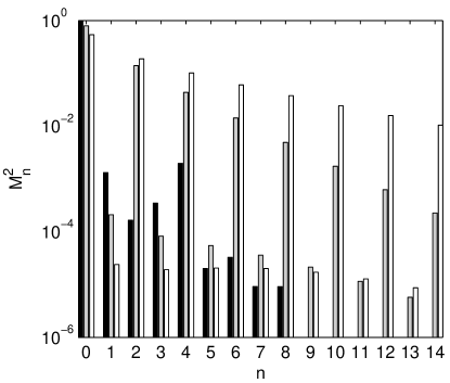
Figure 8: Squared coefficients $M_{n}^{2}$ for the decomposition of a local oscillator pulse given by Eq. (37) into characteristic squeezing modes according to Eq. (33), for the nonlinear length $L_{\mathrm{NL}}=1/2$ mm and $\tau_{\mathrm{LO}}=15$ fs (black bars), $\tau_{\mathrm{LO}}=30$ fs (grey bars), and $\tau_{\mathrm{LO}}=50$ fs (empty bars). Note the logarithmic scale on the vertical axis.

The quadrature noise observed in homodyne detection of multimode squeezed light is similar to that of a single-mode squeezed state with an inefficient detector in that it does not exhibit minimum uncertainty: $\langle Q_{+}^{2}\rangle\langle Q_{-}^{2}\rangle>1/16$. In the latter case, the efficiency of the detector can be calculated as follows:

$$\eta=\frac{-16\langle Q_{+}^{2}\rangle\langle Q_{-}^{2}\rangle+4\langle Q_{+}^{2}\rangle+4\langle Q_{-}^{2}\rangle-1}{4\langle Q_{+}^{2}\rangle+4\langle Q_{-}^{2}\rangle-2}.$$ (38)

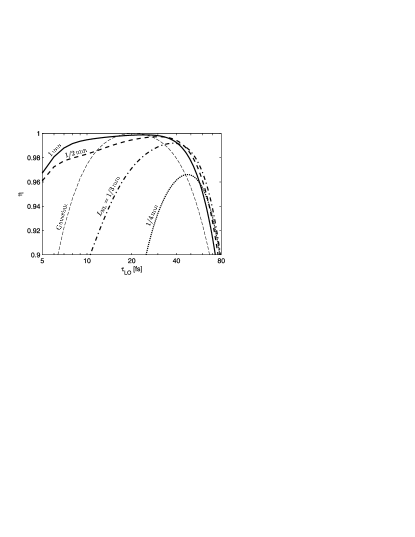
Figure 9: Quantum efficiency $\eta$ of detecting squeezing defined in Eq. (38) as a function of the local oscillator duration $\tau_{LO}$ for nonlinear lengths $L_{\mathrm{NL}}=1$ mm (solid line), $L_{\mathrm{NL}}=1/2$ mm (dashed line), $L_{\mathrm{NL}}=1/3$ mm (dashed-dotted line), and $L_{\mathrm{NL}}=1/4$ mm (dotted line). The thin dashed line represents the result of the Gaussian approximation.

It is sometimes useful to express the quality of multimode squeezed light in terms of the efficiency calculated according to the above relation. In Fig. 9, we plot this quantity for a local oscillator of the shape given by Eq. (37), as a function of the LO pulse duration, for several squeezing strengths. We observe the same general behavior as in Fig. 7. In the single-pair generation regime, high-$\eta$ squeezing detection is possible in a broad span of LO modes within the interval $1/\Delta\leq\tau_{LO}\leq 1/\delta$; as the pumping intensity is increased, the choice of LO becomes a lot more critical.

Most existing experiments on pulsed squeezing derive the local oscillator from the master laser whose second harmonic serves as a pump for the down-conversion. According to Figs. 7 and 9, this is not always the best strategy. In the weak pumping regime, the highest efficiency is achieved for the LO pulse duration of $\tau_{s}$, which is usually much shorter than the fundamental pulse width (30). With increasing squeezing strength, the optimal LO pulse width increases.

Combining these considerations allows one to match the parameters of the setup, such as the duration of the fundamental and second-harmonic pulses, as well as the characteristics of the down-conversion crystal, in order to reach the optimum detection of squeezing.

VI Conclusions

In summary, we have analyzed the spectral properties of pulsed squeezed light generated by means of single-pass optical parametric amplifier. The main tool in our analysis was the Bloch-Messiah decomposition of the Green functions describing the parametric down-conversion process. This decomposition allowed us to identify the characteristic squeezing modes, which provide a simple way of describing quantum statistical properties of the multimode output field.

We have developed an analytical model describing the perturbative regime of single pair generation $L/L_{\mathrm{NL}}\ll 1$, when the nonlinear interaction length $L_{\mathrm{NL}}$ substantially exceeds the crystal length $L$. The model yielded an approximate form of the squeezing modes as well as their characteristic time scale. In this regime, high-efficiency squeezing expands over a broad range of pulsed modes temporally synchronized with the pump pulse. Some of the results of the analytical model, such as the mode shapes, remain qualitatively valid also beyond the perturbative limit.

For the multiple-pair generation case we have presented realistic numerical calculations of the characteristic modes of a parametric amplifier, in which pure squeezing is present. Beyond the perturbative regime, the mode functions depend on the pumping intensity, including the change in their spectral phases. As with increasing parametric gain the fluctuations in antisqueezed quadratures grow exponentially, it becomes more difficult to eliminate their parasitic contribution to the observed homodyne noise. Therefore, one needs precise tailoring of the local oscillator mode, including both its amplitude and its phase, if substantial squeezing is to be observed.

The multimode character of the output field generated by an optical parametric amplifier has important consequences when considering quantum information applications based on continuous variables, such as quantum cryptography. For example, if a quantum communication protocol involves modulating squeezed light, care must be taken to ensure that only the mode detected at the receiving station experiences modulation. Otherwise other modes might carry the same signal and could be detected by a third party without causing any observable disturbance. Furthermore, if the quadrature fluctuations detected by the legitimate user remain above the minimum uncertainty limit, this implies that the observed mode was correlated with other undetected modes which again could be used to gain information by a third party. The multimode nature of pulsed squeezing also needs to be taken into account is quantum state engineering combining discrete- and continuous-variable methods, such as preparation of squeezed single-photon states Sasaki05 ; gran04 , Schrödinger cats lund04 , and entanglement purification cventpur . When multimode squeezing is undesired, it can be prevented by choosing down-conversion configuration with unentangled biphoton spectrum GricePRA01 ; ure05 ; microcavity .

Let us also note that the decomposition of the output of the parametric process into characteristic squeezing modes enables a straightforward analysis of the result of combining two squeezed beams on a balanced beam splitter. It is well known that in the single-mode picture, such a procedure yields a pair of twin beams Ou92 . In the realistic case, if the two incident squeezed beams are generated by identical parametric amplifies, they will comprise the same characteristic squeezing modes perfectly matched pair-wise. Consequently, combining them on a beam splitter will yield multimode twin beam sets which exhibit minimum-uncertainty quadrature correlations in the characteristic modes of the squeezers.

Appendix A Analysis in the interaction picture

The evolution of the quantum state of light while propagating through the crystal follows:

$$\left|\psi_{I}^{out}\right\rangle={\cal T}\exp\left[-i\int\limits_{-L/2}^{L/2}\hat{V}_{I}(z)dz\right]\left|\psi_{I}^{in}\right\rangle,$$ (39)

where the subscript $I$ denotes the interaction picture and ${\cal T}$ denotes $z$-ordering, analogous to standard time ordering. The three-wave mixing Hamiltonian (II) can be rewritten in the interaction picture as

$$\hat{V}_{I}(z)=\frac{1}{2L_{\mathrm{NL}}E_{0}}\int d\omega\,d\omega^{\prime}$$

$$\times[ie^{i\Delta kz}E_{p}(\omega^{\prime}+\omega)\hat{a}^{\dagger}(\omega)\hat{a}^{\dagger}(\omega^{\prime})+{\rm H.c.}],$$

where $\Delta k$ is given by Eq. (20). In the weak conversion limit, when only the first order of the perturbation theory is relevant, we can neglect the $z$-ordering and obtain

$$\left|\psi_{I}^{out}\right\rangle=e^{\frac{1}{2}\int d\omega d\omega^{\prime}\Psi_{I}(\omega,\omega^{\prime})[\hat{a}^{\dagger}(\omega)\hat{a}^{\dagger}(\omega^{\prime})-\hat{a}(\omega)\hat{a}(\omega^{\prime})]}\left|\psi_{I}^{in}\right\rangle,$$ (41)

where the integration kernel

$$\Psi_{I}(\omega,\omega^{\prime})=\frac{LE_{p}(\omega+\omega^{\prime})}{L_{\mathrm{NL}}E_{0}}\,\,\mathrm{sinc}\frac{L\Delta k}{2}\\$$

determines the frequency correlations of photons in a down-converted pair. In the weak excitation limit with the vacuum input, the output state takes the form:

$$\left|\psi_{I}^{out}\right\rangle=\left|0\right\rangle+\frac{1}{2}\int d\omega d\omega^{\prime}\Psi_{I}(\omega,\omega^{\prime})\left|1_{\omega},1_{\omega^{\prime}}\right\rangle.$$ (42)

In the Schrödinger picture, the output state acquires an additional optical phase:

$$\Psi_{S}(\omega,\omega^{\prime})=\Psi_{I}(\omega,\omega^{\prime})e^{i[k(\omega)+k(\omega^{\prime})]L/2}.$$ (43)

We recover Eq. (23) from Eqs. (LABEL:S'1st), (A), and (43).

Note that the biphoton spectrum can be diagonalized according to Eq. (14)

$$\Psi_{S}(\omega,\omega^{\prime})=\sum\limits_{n=0}^{\infty}\zeta_{n}\psi_{n}(\omega)\psi_{n}(\omega^{\prime}).$$ (44)

and the output state can be rewritten as follows:

$$\left|\psi_{S}^{out}\right\rangle=\left|0\right\rangle+\frac{1}{2}\sum\limits_{n=0}^{\infty}\zeta_{n}(\hat{b}_{n}^{out\,\dagger})^{2}\left|0\right\rangle,$$ (45)

where the $\hat{b}_{n}$’s represent individual squeezing eigenmodes (10). As we see, the problem of finding the characreristic modes of a squeezer in the weak pumping limit is equivalent to decomposing the biphoton spectrum into uncorrelated components.

References

- (1) R. E. Slusher, L. W. Hollberg, B. Yurke, J. C. Mertz, and J. F. Valley, Phys. Rev. Lett. 55, 2409 (1985).
- (2) L.-A. Wu, H. J. Kimble, J. L. Hall, and H. Wu, Phys. Rev. Lett. 57, 2520 (1986).
- (3) P. Grangier, R. E. Slusher, B. Yurke and A. LaPorta, Phys. Rev. Lett. 59, 2153 (1987).
- (4) H. P. Yuen and J. H. Shapiro, IEEE Trans. Inform. Theory IT25, 179 (1979); J. H. Shapiro, Opt. Lett. 5, 351 (1980).
- (5) Z. Y. Ou, S. F. Pereira, H. J. Kimble, and K. C. Peng, Phys. Rev. Lett. 68, 3663 (1992).
- (6) A. Furusawa, J. L. Sorensen, S. L. Braunstein, C. A. Fuchs, H. J. Kimble, and E. S. Polzik, Science 282, 706 (1998).
- (7) S. Lloyd and S. L. Braunstein, Phys. Rev. Lett. 82, 1784 (1999).
- (8) T. C. Ralph, Phys. Rev. A 61, 010303 (2000).
- (9) A. Kuzmich and E. S. Polzik, Phys. Rev. Lett. 85, 5639 (2000).
- (10) S. L. Braunstein, Nature 394, 74 (1998).
- (11) S. Lloyd and J. J.-E. Slotine, Phys. Rev. Lett. 80, 4088 (1998).
- (12) L.-M. Duan, G. Giedke, J. I. Cirac, and P. Zoller, Phys. Rev. A 62, 032304 (2000).
- (13) D. E. Browne, J. Eisert, S. Scheel, and M. B. Plenio, Phys. Rev. A 67, 062320 (2003).
- (14) R. E. Slusher, P. Grangier, A. LaPorta, B. Yurke and M. J. Potasek, Phys. Rev. Lett. 59, 2566 (1987).
- (15) P. Kumar, O. Aytur and J. Huang, Phys. Rev. Lett. 64, 1015 (1990).
- (16) D. T. Smithey, M. Beck, M. G. Raymer and A. Faridani, Phys. Rev. Lett. 70, 1244 (1993).
- (17) C. Kim and P. Kumar, Phys. Rev. Lett. 73, 1605 (1994).
- (18) M. E. Anderson, M. Beck, M. G. Raymer and J. D. Bierlein, Opt. Lett. 20, 620 (1995).
- (19) E. M. Daly, A. S. Bell, E. Riis and A. I. Ferguson, Phys. Rev. A 57, 3127 (1998).
- (20) M. Sasaki and S. Suzuki, quant-ph/0512073
- (21) S. L. Braunstein, Phys. Rev. A 71, 055801 (2005); For a treatment based on hermitian (quadrature) observables, see Arvind, B. Duta. N. Mukunda, and R. Simon, Pramana-J. Phys. 45, 471 (1995).
- (22) R.S. Bennink, R.W. Boyd, Phys. Rev. A 66, 053815 (2002).
- (23) X. Mia and W. Rhodes, Phys. Rev. A 41, 4625 (1990).
- (24) R. W. Boyd Nonlinear Optics, Academic Press, Boston, 1992.
- (25) T. E. Keller and M. H. Rubin, Phys. Rev. A 56, 1534 (1997).
- (26) W. P. Grice and I. A. Walmsley, Phys. Rev. A 56, 1627 (1997).
- (27) C. K. Law, I. A. Walmsley, and J. H. Eberly, Phys. Rev. Lett. 84, 5304 (2000).
- (28) M. J. Werner, M. G. Raymer, M. Beck and P. D. Drummond, Phys. Rev. A 52, 4202 (1995).
- (29) J. H. Shapiro and A. Shakeel, J. Opt. Soc. Am. B 14, 232 (1997).
- (30) M. Yamada, N. Nada, M. Saitoh, and K. Watanabe, Appl. Phys. Lett. 62, 435 (1993).
- (31) Y.B. Band, C. Radzewicz, and J.S. Krasiński, Phys. Rev. A 49, 517 (1994).
- (32) An experimental approach to spatial separation of nonmonochromatic modes into a distinct spatial channels in order to remove correlations for input Gaussian fields has been proposed in T. Opatrný, N. Korolkova and G. Leuchs, Phys. Rev. A 66, 053813 (2002).
- (33) D. T. Smithey, M. Beck, M. Belsley, and M. G. Raymer, Phys. Rev. Lett. 69, 2650 (1992)
- (34) J. Perina, Jr., A. V. Sergienko, B. M. Jost, Bahaa E. A. Saleh, and M. C. Teich, Phys. Rev. A 59, 2359 (1999).
- (35) W. P. Grice, A. B. U’Ren and I. A. Walmsley, Phys. Rev. A 64, 063815 (2001).
- (36) The opposite case has been recently implemented in O. Kuzucu et al., Phys. Rev. Lett. 94, 083601 (2005)
- (37) K. Banaszek and K. Wódkiewicz, Acta Phys. Slov. 49, 491 (1999).
- (38) Our scaling convention is .
- (39) J. Wenger, R. Tualle-Brouri, and P. Grangier, Phys. Rev. Lett. 92, 153601 (2004)
- (40) A.P. Lund, H. Jeong, T.C. Ralph, M.S. Kim, Phys. Rev. A 70, 020101 (2004)
- (41) D. E. Browne, J. Eisert, S. Scheel, and M. B. Plenio, Phys. Rev. A 67, 062320 (2003);
- (42) A. B. U’Ren et al., Laser Phys. 15, 146 (2005)
- (43) Raymer, M. G., J. Noh, K. Banaszek, and I.A. Walmsley, Phys. Rev. A 72, 023825 (2005).