Infinite qubit rings with maximal nearest neighbor entanglement: the Bethe ansatz solution

Abstract

We search for translationally invariant states of qubits on a ring that maximize the nearest neighbor entanglement. This problem was initially studied by O’Connor and Wootters [Phys. Rev. A 63, 052302 (2001)]. We first map the problem to the search for the ground state of a spin 1/2 Heisenberg XXZ model. Using the exact Bethe ansatz solution in the limit $N\rightarrow\infty$, we prove the correctness of the assumption of O’Connor and Wootters that the state of maximal entanglement does not have any pair of neighboring spins “down” (or, alternatively spins “up”). For sufficiently small fixed magnetization, however, the assumption does not hold: we identify the region of magnetizations for which the states that maximize the nearest neighbor entanglement necessarily contain pairs of neighboring spins “down”.

I Introduction

The investigation of the role of entanglement in quantum and classical phase transitions, and more generally the role of entanglement in many-body quantum systems is one of the hottest interdisciplinary areas on the borders between quantum information, quantum optics, atomic, molecular, and condensed matter physics. Initially the studies of entanglement in many-body systems have been motivated by the possibility of employing entanglement for quantum computation in optical lattices optical_lattice , or precision measurements with Bose-Einstein condensates BEC . Recently, several lines of research have been followed:

• Studies of local entanglement in spin systems Osterloh ; Nielsen ; salikh-qwerty ; salikh-qwerty1 ; Indranidi , and more generally in various many-body systems (such as linear chains, see for instance linchain ; Bogol ; wolflin ), with particular attention to the role of entanglement in phase transitions.

• Studies of the entropy of blocks of spins and the related “area law” area1 , indicating weak entanglement of blocks, and effects of criticality salikh-qwerty ; area2 ; wolflin ; meti-pukur .

• Studies of localisable entanglement and entanglement correlation length that diverges at the critical point ent_length ; Ciracnew and majorizes the standard correlation length (see also kachpoka ). In particular, it has been shown that the localisable entanglement (cf. hmmmm ; amrao-achhi-re-bhai ; jin04:_localiz_entang_spin_chain ) is bounded from above by the entanglement of assistance Bennett-assistance and from below by correlation functions. It follows directly from these bounds that one can define an entanglement correlation length that diverges in quantum critical systems.

• Studies of multipartite entanglement in many-body systems Dagmar .

• Studies of dynamics and generation of entanglement in many-body systems Briegel_orey_orey ; Sougato ; talk_dilo_Osterloh ; amader ; meti-pukur . In particular, implementations of the “one-way quantum computer” and short range teleportation BBCJPW of an unknown state has been proposed by using the dynamics of spin systems in Refs. Briegel_orey_orey ; Briegel_ebong ; meti-pukur ; Sougato ; Sougato_ebong ; dpt .

• Studies of quantum information and entanglement theory inspired numerical codes to simulate quantum systems numerical .

A different approach to the study of entanglement in many-body systems has been proposed in two papers by Wootters and coworkers Wootters . In these papers, instead of looking at a specific Hamiltonian, the authors asked the fundamental question “what is the maximal entanglement between two neighboring sites of an entangled ring with translational invariance?” Here, an entangled ring is a chain of spins with periodic boundary conditions. Due to the so-called “monogamy of entanglement” it is impossible for a site to be maximally entangled with both its neighbors: shared entanglement is always less than maximal brusspra ; oldwootters . In Ref. Wootters the question of the upper limit for the nearest neighbor (NN) entanglement was simplified by introducing two additional restrictions on the allowed states:

• The state of $N$ spins 1/2 is an eigenstate of the $z$-component of the total spin (i.e. it has a fixed number of “down” spins $p\leq N/2$) .

• Neighboring spins cannot both be “down”.

Obviously, one can equally well study the same problem in terms of spins “up”, when $N\geq p\geq N/2$. Both restrictions are based on an educated guess for the optimal states for the general problem. O’Connor and Wootters (OW) solved the restricted optimization problem by relating it to an effective Hamiltonian for the one-dimensional ferromagnetic XY model, and found the maximal nearest-neighbor concurrence (cf. Sec. II) for given $N$ and $p$ to be

$$C^{\text{max}}_{\text{OW}}(N,p)=\frac{2\sin\left(\frac{p\pi}{N-p}\right)}{N\sin\left(\frac{\pi}{N-p}\right)}\;.$$ (1)

For given $N$ and $p$, Eq. (1) provides a lower bound for the problem without restriction (ii). It may, or may not happen that $C$ can be increased by also allowing states where two neighboring spins are “down”. We have recently studied finite size rings and found that for a fixed $p$ restriction (ii) tends to play a less important role as $N$ is increased meyer : For $p$ close to $N/2$ one can increase the concurrence significantly by dropping restriction (ii), but for $p\lesssim N/3$ OW’s result is the optimal one. In fact, already in Ref. Wootters it was shown that for all even $N$ the ground state of a Heisenberg spin 1/2 antiferromagnetic ring maximizes the concurrence among the zero magnetization ($p=N/2$) states although it violates restriction (ii).

By optimizing (1) with respect to $p$ one obtains a lower bound on the overall optimal concurrence, i.e. without any restrictions besides the translational invariance. In the limit $N\rightarrow\infty$, the optimal number of spins “down” in Eq. (1) approaches $p_{\text{opt}}\approx 0.301\;N$. This leads to an asymptotic value of $C_{\text{OW}}^{\text{max}}\approx 0.434$. Although Ref. Wootters as well as our previous work meyer showed evidence for optimality of this number, whether it can be improved was, so far, an open problem.

Wolf, Verstraete, and Cirac have in Ref. wolf03:_entan_frust directly related OW’s type of problems of looking for translationally invariant states that maximize local entanglement to the study of the ground state of a suitably defined “parent” Hamiltonian. In this paper we use this method and employ the known exact solution of the corresponding parent Hamiltonian to prove rigorously that:

• In the limit $N\to\infty$ the translationally invariant state that maximizes the NN entanglement without any restriction coincides with the state found by OW at the optimal value of $p\simeq 0.301N$. This means that it is not a superposition of states with different $p$ values and does not contain simultaneously neighboring spin “up” and neighboring spin “down” pairs.

• For fixed $p$ sufficiently close to $N/2$, i.e. for sufficiently small magnetizations, assumption (ii) is not correct: the states that maximize the nearest neighbor entanglement necessarily contain simultaneously pairs of neighboring “up” and “down” spins. In the limit $N\rightarrow\infty$ we identify rigorously an interval of $p/N$ for which this is the case and show strong numerical evidence that this interval is optimal.

Our paper is organized as follows. In Section II we apply the method of Ref. wolf03:_entan_frust and derive the corresponding parent Hamiltonian for a $N$ qubit ring. In Section III we show the connection with the “classical” papers of Yang and Yang on the XXZ model. In Section IV we discuss briefly the regimes of parameters of interest and show that the present problem concerns the “difficult” parameter region of the phase diagram. In Section V we present the analysis based on the limit $N\to\infty$ of the Bethe ansatz solutions. We derive here the basic integral equation, the solution of which allows to calculate the desired energy of the system in question. In Section VI the numerical results are discussed. In Section VII we rigorously prove that the states that were conjectured in Ref. Wootters to maximize the NN entanglement and confirmed by us, indeed provide the maximum of the NN entanglement for sufficiently small values of $p$. We identify the region of $p/N$ where the latter statement does not hold. We conclude in Section VIII. The short appendix contains simple analytic bounds on optimal magnetic field for which the NN concurence is maximal.

II Variational concurrence formula

In this paper we will use the concurrence as our entanglement measure. The concurrence defconc is defined as $C(\rho)=\max\{\lambda_{1}-\lambda_{2}-\lambda_{3}-\lambda_{4},0\}$, where $\lambda_{1}\geq\lambda_{2}\geq\lambda_{3}\geq\lambda_{4}\geq 0$ are the square roots of the eigenvalues of $\rho\tilde{\rho}$, and $\tilde{\rho}=(\sigma_{y}\otimes\sigma_{y})\rho^{*}(\sigma_{y}\otimes\sigma_{y})$ is the spin-flipped density matrix. The optimization problems that we consider are complicated by the nonlinearity of the concurrence as function of the density matrix. In our previous work meyer , we showed how the optimization problem with fixed $p$ can be reformulated as finding the ground state energy for each in a family of spin-chain Hamiltonians. This family is parameterized by a single real parameter and the optimal concurrence is minus the lowest ground state energy that occurs when this parameter is varied. In this way a complicated non-linear problem in a high-dimensional space is replaced by a series of linear problems and one final one-parameter optimization.

The derivation in Ref. meyer did not cover the case where superpositions of states with different $p$ are allowed. To treat that case, we turn to Ref. wolf03:_entan_frust where the following general formula for the concurrence for systems of two spins $1/2$ has been derived:

$$C(\rho)=\max\left\{0,-\inf_{\det X=1}\mathrm{tr}\left[\rho\left(X\otimes X^{\dagger}\mathbf{F}\right)\right]\right\}.$$ (2)

Here $X$ is an arbitrary $2\times 2$ matrix of determinant 1, while $\mathbf{F}$ is the flip (or swap) operator, interchanging the two qubits:

$$\mathbf{F}=|\!\!\uparrow\uparrow\rangle\!\langle\uparrow\uparrow\!\!|+|\!\!\downarrow\downarrow\rangle\!\langle\downarrow\downarrow\!\!|+|\!\!\downarrow\uparrow\rangle\!\langle\uparrow\downarrow\!\!|+|\!\!\uparrow\downarrow\rangle\!\langle\downarrow\uparrow\!\!|.$$ (3)

A useful parameterization of $X$ is obtained using the singular value decomposition horn85:_matrix_analysis :

$$X=U\begin{bmatrix}it&0\\ 0&\frac{1}{it}\end{bmatrix}V^{\dagger},$$ (4)

where $t\in[-\infty,\infty]$, $U,V\in U(2)$ and $\det U\cdot\det V^{\dagger}=1$. In fact, from Eq. (2) it is clear that we can restrict to $U,V\in SU(2)$. We now rewrite

$$X\otimes X^{\dagger}\;\mathbf{F}\\ =\left(U\otimes V\right)\left(\begin{bmatrix}it&0\\ 0&\frac{1}{it}\end{bmatrix}\otimes\begin{bmatrix}-it&0\\ 0&\frac{1}{-it}\end{bmatrix}\right)\left(V^{\dagger}\otimes U^{\dagger}\right)\mathbf{F}\\ =\left(U\otimes V\right)\begin{bmatrix}t^{2}&0&0&0\\ 0&-1&0&0\\ 0&0&-1&0\\ 0&0&0&t^{-2}\end{bmatrix}\mathbf{F}\left(U\otimes V\right)^{\dagger}\\ =\left(U\otimes V\right)\begin{bmatrix}t^{2}&0&0&0\\ 0&0&-1&0\\ 0&-1&0&0\\ 0&0&0&t^{-2}\end{bmatrix}\left(U\otimes V\right)^{\dagger}.$$ (5)

Let us define the matrix in square brackets as $h(t^{2})$, i.e.,

$$h(s)=s|\!\!\uparrow\uparrow\rangle\!\langle\uparrow\uparrow\!\!|+\frac{1}{s}|\!\!\downarrow\downarrow\rangle\!\langle\downarrow\downarrow\!\!|-|\!\!\downarrow\uparrow\rangle\!\langle\uparrow\downarrow\!\!|-|\!\!\uparrow\downarrow\rangle\!\langle\downarrow\uparrow\!\!|.$$ (6)

where $s=t^{2}$. Then we can rewrite Eq. (2) as

$$C(\rho)=\\ \max\left\{0,-\inf_{s,U,V}\mathrm{tr}\left[\left(U\otimes V\right)^{\dagger}\rho\left(U\otimes V\right)h(s)\right]\right\}.$$ (7)

Our goal is to maximize the concurrence over all $\rho$ that can occur as nearest neighbor density matrices on a translationally invariant ring. If we always had $U=V$, it is easy to see that we could drop the infimum over $U\in SU(2)$ in Eq. (7) since if $\rho=\mathrm{tr}_{3\ldots N}\Gamma$ with $\Gamma$ translationally invariant then $(U\otimes U)^{\dagger}\rho(U\otimes U)=\mathrm{tr}_{3\ldots N}(U\otimes\ldots\otimes U)^{\dagger}\Gamma(U\otimes\ldots\otimes U)$ where $(U\otimes\ldots\otimes U)^{\dagger}\Gamma(U\otimes\ldots\otimes U)$ is translationally invariant as well. To do the same for $U\neq V$, we can use the fact that $h(s)$ is symmetric in the two qubits:

$$\mathrm{tr}\left[\left(U\otimes V\right)^{\dagger}\rho\left(U\otimes V\right)h(s)\right]=\mathrm{tr}\left[\tilde{\rho}h(s)\right]$$ (8)

where

$$\tilde{\rho}=\\ \frac{1}{2}\left\{\left(U\otimes V\right)^{\dagger}\rho\left(U\otimes V\right)+\left(V\otimes U\right)^{\dagger}\rho\left(V\otimes U\right)\right\}.$$ (9)

If $N$ is even and $\rho=\mathrm{tr}_{3\ldots N}\Gamma$ then $\tilde{\rho}$ is a nearest neighbor density matrix belonging to the following translationally invariant state:

$$\begin{split}\frac{1}{2}\bigg{\{}&\phantom{+}\left([U\otimes V]\otimes\ldots\otimes[U\otimes V]\right)^{\dagger}\times\\ &\phantom{aabbccdd}\times\Gamma\times\left([U\otimes V]\otimes\ldots\otimes[U\otimes V]\right)\\ &+\left([V\otimes U]\otimes\ldots\otimes[V\otimes U]\right)^{\dagger}\times\\ &\phantom{aaccbbdd}\times\Gamma\times\left([V\otimes U]\otimes\ldots\otimes[V\otimes U]\right)\bigg{\}}.\end{split}$$ (10)

If $N$ is odd, the above construction does not work: we cannot fit an integer number of $U\otimes V$ terms on the ring. By placing as many terms $U\otimes V$ as possible, and taking the translationally variant mixture of the resulting state, $\tilde{\rho}$ can be approximated up to a factor $1/N$. In the limit of $N\rightarrow\infty$ we can ignore this correction.

III The parent Hamiltonian

In this section we will follow the approach of Ref. wolf03:_entan_frust to derive the parent spin $1/2$ XXZ Hamiltonian, i.e. the Hamiltonian whose ground state maximizes the NN concurrence. We also make the connection to the classical papers on the XXZ model by Yang and Yang yang66:_one_dimen_I ; yang66:_one_dimen_II ; yang66:_one_dimen_III .

In the previous section we showed that in the limit $N\rightarrow\infty$

$$C^{\text{max}}(N)=\max_{\rho}C(\rho)=-\inf_{s,\rho}\mathrm{tr}[\rho h(s)]$$ (11)

where $\rho=\mathrm{tr}_{3\ldots N}\Gamma$ for some translationally invariant $\Gamma$ of $N$ spins. The two-spin Hamiltonian (6) can be written in terms of Pauli matrices as

$$\begin{split}h(s)=&\frac{s}{4}\left(\mathbf{1}+\sigma_{z}\right)\left(\mathbf{1}+\sigma_{z}\right)+\frac{1}{4s}\left(\mathbf{1}-\sigma_{z}\right)\left(\mathbf{1}-\sigma_{z}\right)\\ &-\sigma_{+}\sigma_{+}-\sigma_{-}\sigma_{-}\\ =&\frac{1}{2}\left\{-\sigma_{x}\sigma_{x}-\sigma_{y}\sigma_{y}+\frac{1}{2}\left(s+\frac{1}{s}\right)\left(\sigma_{z}\sigma_{z}+1\right)\right.\\ &\left.+\frac{1}{2}\left(s-\frac{1}{s}\right)\left(\sigma_{z}\mathbf{1}+\mathbf{1}\sigma_{z}\right)\right\},\end{split}$$ (12)

where $\sigma_{\pm}=\sigma_{x}\pm i\sigma_{y}$. Instead of working with $\rho$ and $h(s)$ we can use the translational invariance and work with $\Gamma$ and a Hamiltonian for the whole ring obtained by taking (12) for each NN pair:

$$\begin{split}H_{\text{Wolf}}(s)&=\\ \frac{1}{2N}&\sum_{i=1}^{N}\big{\{}-\sigma_{x}^{i}\sigma_{x}^{i+1}-\sigma_{y}^{i}\sigma_{y}^{i+1}-\Delta(s)\sigma_{z}^{i}\sigma_{z}^{i+1}\\ &\phantom{\sum_{i=1}^{N}\big{\{}-\sigma_{x}^{i}\sigma_{x}^{i+1}}-2\mathcal{H}(s)\sigma_{z}^{i}-\Delta(s)\big{\}},\end{split}$$ (13)

where

$$\Delta(s)=-\frac{1}{2}\left(s+\frac{1}{s}\right)\qquad\mathcal{H}(s)=-\frac{1}{2}\left(s-\frac{1}{s}\right).$$ (14)

We have then reformulated the overall optimization problem as

$$C^{\text{max}}(N)=\max_{\rho}C(\rho)=-\inf_{s,\Gamma}\mathrm{tr}[\Gamma H_{\mathrm{Wolf}}(s)],$$ (15)

where $\rho$ is restricted to arise from a translationally invariant state of $N$ spins while the optimal $\Gamma$ can automatically be chosen so since $H_{\mathrm{Wolf}}$ is translationally invariant.

An important observation can be made from Eq. (15), namely that as $H_{\mathrm{Wolf}}$ commutes with the $z$ component of the total spin, in the considered limit of $N\rightarrow\infty$ OW were right when they made assumption (i): The optimal state can indeed be chosen to have a definite number of spins “down” and thus does not contain superpositions of states with different $p$ values. Conversely, from our previous work meyer we know that Eq. (15) is also valid for any fixed $p$, i.e. we can write $C^{\text{max}}(N,p)$ on the left-hand side when making the appropriate restrictions on $\Gamma$. In summary, for fixed $p$ the maximal concurrence is given by:

$$C^{\text{max}}(N,p)=-\inf_{s}E_{\text{GS}}[H_{\text{Wolf}}(s),p],$$ (16)

where $E_{\text{GS}}[H_{\text{Wolf}}(s),p]$ is the “ground state” energy of $H_{\text{Wolf}}(s)$ in the manifold of states with $p$ spins “down”. The overall maximal concurrence is given by further optimization over $p$ or, equivalently, by using unrestricted ground state energies:

$$\begin{split}C^{\text{max}}(N)&=\max_{p}C^{\text{max}}(N,p)\\ =&-\inf_{s}E_{\text{GS}}[H_{\text{Wolf}}(s)].\end{split}$$ (17)

Let us now describe the connection with the work of Yang and Yang. In their seminal papers Yang and Yang yang66:_one_dimen_I ; yang66:_one_dimen_II ; yang66:_one_dimen_III study this anisotropic Heisenberg XXZ Hamiltonian (see e.g. korepin93:_quant_inver_scatt for more recent work):

$$H_{\text{Yang}}=-\frac{1}{2}\sum_{i}\left\{\sigma_{x}^{i}\sigma_{x}^{i+1}+\sigma_{y}^{i}\sigma_{y}^{i+1}+\Delta\sigma_{z}^{i}\sigma_{z}^{i+1}\right\},$$ (18)

and they define $f=\lim_{N\rightarrow\infty}f_{N}$, where $f_{N}$ is half the energy per spin in the ground state with a given number $p$ of spins “down”:

$$f_{N}(\Delta,y)=\frac{1}{2N}E_{\text{GS}}(H_{\text{Yang}},p).$$ (19)

Here $y$ is the average magnetization:

$$y=\frac{1}{N}\langle\sum\sigma_{z}^{i}\rangle=1-\frac{2p}{N}.$$ (20)

Since $p$ is a conserved quantum number, one can include a magnetic field along $z$ and only shift the energy of each eigenstate. The translation of the results of Yang and Yang to our optimization problems is therefore,

$$E_{\text{GS}}[H_{\text{Wolf}}(s),p]=\\ 2f_{N}(\Delta(s),y)-\mathcal{H}(s)y-\frac{1}{2}\Delta(s),$$ (21)

with $s>0$. Note that $\Delta^{2}-\mathcal{H}^{2}=1$. To find $C^{\text{max}}(N,p)$ we should minimize Eq. (21) over $s$ while keeping $y$ fixed at the value corresponding to $p$ [cf. Eq. (20)]. To find the overall maximal concurrence $C^{\text{max}}(N)$ we should furthermore minimize over $y$.

IV The phase-diagram of the XXZ model

We are considering the XXZ model in the limit $N\rightarrow\infty$. The second Yang and Yang paper yang66:_one_dimen_II deals with the properties of $f(\Delta,y)$ in exactly this limit. The third paper yang66:_one_dimen_III contains information about the magnetic properties, i.e. it is highly relevant when we also vary $y$ in order to find the optimal fraction of spins “down”.

Figure 1: Phase diagram for the XXZ chain in a magnetic field. For large negative $\Delta$ and small magnetic field $\mathcal{H}$ the ground state has perfect anti-ferromagnetic ordering (AF) with vanishing magnetization. When the magnetic field is increased beyond a certain critical value (lower bold line in the plot), a non-vanishing magnetization develops. The magnetization increases with increasing field until finally all the spins are aligned. This aligned phase (A) is entered at an upper critical field indicated by the upper fat line in the plot. We are interested in the properties of the chain along the dashed line in the plot, i.e. we deal with the phase with non-vanishing, but also non-saturated magnetization.

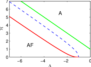
In order to understand the regimes of parameters we are interested in and relate them to the known properties of the model, it is useful to look at the phase diagram of this model, displayed in Fig. 1.

Let us first identify the region of the phase diagram which belongs to our parent Hamiltonian (13). From Eq. (14) it is clear that as $s$ varies from $0$ to $\infty$, we move on a hyperbola in the $\Delta$–$\mathcal{H}$ plane: The $s=0$ case corresponds to $(-\infty,\infty)$, whereas at $s=1$ we are at the point of closest approach and cross the $\Delta$ axis in $(-1,0)$, and as $s\rightarrow\infty$ we move back to infinity, but this time with negative magnetic field. Comparing this with Fig. 1, it is then easy and not surprising to see that the $s$-hyperbola lies exactly in the “difficult” region of the phase diagram, i.e., the part with neither perfectly aligned spins nor perfect anti-ferromagnetic order (between AF and A in Fig. 1).

Since a change of sign of the magnetic field will only interchange the role of spin “up” and spin “down”, we can ignore the negative $\mathcal{H}$ branch and focus on $s\in[0,1]$. Then each point on the curve corresponds to exactly one $\Delta$ and we can thus parameterize the curve by $\Delta$ instead of $s$. The optimization is then done over $\Delta$ with the magnetic field always given by $\mathcal{H}=\sqrt{\Delta^{2}-1}$.

V The integral equation

The Bethe ansatz basically consists of the assumption that the wave function can be written as a sum of plane waves with a limited number of terms. If we are looking for a state with $p$ spins “down”, only $p$ wave numbers are needed. For the XXZ chain the first Yang and Yang article shows that this is indeed enough to produce the ground state wave function yang66:_one_dimen_I . For our purposes we should note that Yang and Yang give explicitly the equations one needs to solve in order to find the ground state energy. In the limit of $N\rightarrow\infty$, the number of wave numbers naturally becomes infinite and the equation to find them becomes an integral equation for the wave number density. This equation mathematically has a form of a so called Fredholm equation of the second kind. After some reparameterization this equation attains the form (Eq. [7a] in Ref. yang66:_one_dimen_II ):

$$R(\alpha)=\frac{dp}{d\alpha}-\frac{1}{2\pi}\int_{-b}^{b}\frac{\partial\theta}{\partial\beta}R(\beta)d\beta.$$ (22)

The unknown function here is $R$, which is the reparameterized density of wave numbers. The other functions depend parametrically on $\Delta$, and in terms of the parameter $\lambda=\cosh^{-1}(-\Delta)$, they are explicitly given by:

$$\frac{dp}{d\alpha} =\frac{\sinh\lambda}{\cosh\lambda-\cos\alpha},$$ (23)

$$\frac{\partial\theta}{\partial\beta} =\frac{\sinh 2\lambda}{\cosh 2\lambda-\cos(\alpha-\beta)}.$$ (24)

Let us point out the importance of the integration limit $b$ in Eq. (22): When varying $b$, we get solutions corresponding to different values of $y$. In fact, $y$ is given by:

$$\pi(1-y)=\int_{-b}^{b}R(\alpha)d\alpha.$$ (25)

Note, however, that $R$ also depends on $b$, so the connection is not very obvious. In praxis (i.e. when doing numerics) one solves Eq. (22) for a range of the parameter $b$ in order to find the result for the wanted values of $y$. If one wants to optimize some quantity with respect to $y$, however, this can equally well be achieved by optimizing with respect to $b$.

We are not primarily interested in $R$ (which describes the state), but in $f$, which is the energy. It is given by:

$$f(\Delta,y)=-\frac{\Delta}{4}-\frac{\sinh\lambda}{2\pi}\int_{-b}^{b}R(\alpha)\frac{dp}{d\alpha}d\alpha.$$ (26)

Again, $f$ is written as a function of $y$, but in praxis the dependence is via $b$.

VI Numerical solution of the integral equation

A possible way to solve Eq. (22) is to turn the integral into a sum so that it becomes a matrix equation. This is called the Nystrom method . The best way to discretize an integral is not always equally spaced points; very often it is much more efficient to use a Gaussian Quadrature. This means that we evaluate the integrand at $M$ points $\{\alpha_{k}\}$ and make a weighted sum with weights $\{w_{k}\}$. The points and the weights can be easily found in e.g. Mathematica. In this way, Eq. (22) becomes:

$$R_{k}=\xi_{k}-\sum\limits_{l}w_{l}K_{kl}R_{l}$$ (27)

where

$$R_{k}=R(\alpha_{k})\quad,\quad\xi_{k}=\frac{\sinh\lambda}{\cosh\lambda-\cos\alpha_{k}},$$ (28)

while

$$K_{kl}=\frac{1}{2\pi}\frac{\sinh 2\lambda}{\cosh 2\lambda-\cos(\alpha_{k}-\alpha_{l})}.$$ (29)

It is clear that Eq. (27) is a matrix equation and that solving it cannot be harder than inverting $\mathbf{1}+\tilde{K}$ where $\tilde{K}_{kl}=w_{l}K_{kl}$ (no summation over $l$).

The advantage of using Gaussian Quadrature is that one does not need too many points to get a very good estimate of the integral for any sensible function. What exactly a “sensible function” is depends on the exact Gaussian Quadrature rule used. We use the simple Gauss-Legendre rule, assuming that $R$ is well approximated by a polynomial on the interval $[-b,b]$. This is reasonable here because (23) and (24) are well-behaved for the values of $\lambda$ we will consider. The final matrix equation can be solved very rapidly on a small size computer. A moderate value of $M$, however, means that our knowledge of $R$ is restricted to a rather crude sampling; fortunately this is not a problem, since $y$ and $f$ are themselves integrals, and so can be evaluated with the full accuracy of Gaussian Quadrature.

To give the reader an idea about the numerics, we note that a simple Mathematica program will work very well with $M\leq 30$. To produce a plot $f(\Delta,y)$ versus $y$ for $\Delta$ not too close to $-1$ it takes about one minute. To plot the function of main interest, Eq. (21) optimized over $p$ (i.e. $y$, i.e. $b$) also only takes a few minutes. In Fig. 2 we present the results of a Fortran program, which is (not surprisingly) much faster than the initial Mathematica code. The results indicate that OW’s assumption (ii) was correct: When we plot $E_{\text{GS}}[H_{\text{Wolf}}]$ as function of $\Delta$, we see that the optimal value of $\Delta$ is reached at $-\infty$, and in this limit OW’s result is recovered. We conclude that these simple numerical results indicate that the state that maximizes the NN concurrence without any restrictions (i.e. optimized over $p/N$, i.e. $y$) coincides with the OW state fulfilling assumption (ii) (no NN pairs of spins “down”).

Figure 2: We plot $-E_{\text{GS}}[H_{\text{Wolf}}]$, that is, for each $\Delta$ the optimal $y$ is chosen. It can be seen that the maximum is attained in the limit $\Delta\rightarrow-\infty$ and that the limiting value coincides with OW’s result indicated by the dashed line.

VII Perturbative calculation

Looking at Eq. (21) above we see that the finite value in Fig. 2 in the limit $\Delta\rightarrow-\infty$ is obtained because some diverging terms happen to cancel each other. This is of course a great concern when doing numerics since it means that a good relative precision (knowing the result to e.g. 1 ppm) may not be enough. The obvious strategy is to extract the solution in the strict limit $\Delta\rightarrow-\infty$. In this section, we will present a perturbative calculation in $1/\Delta$.

In zeroth order of the perturbation series we set $\cosh\lambda=\infty$ in Eq. (22), and arrive at the simple equation:

$$R_{0}(\alpha)=1-\frac{1}{2\pi}\int_{b}^{b}R_{0}(\beta)\;d\beta.$$ (30)

The right hand side does not depend on $\alpha$ and we easily find the constant solution:

$$R_{0}=\frac{1}{1+\frac{b}{\pi}}\quad\text{and}\quad y_{0}=\frac{1-\frac{b}{\pi}}{1+\frac{b}{\pi}}.$$ (31)

This means that in this limit $f=-\Delta f_{-1}$ with:

$$f_{-1}=\frac{1}{4}-\frac{\frac{b}{\pi}}{1+\frac{b}{\pi}}=-\frac{1}{4}+\frac{1}{2}y_{0}$$ (32)

and that Eq. (21) thus gives 0, independently of $y_{0}$. At this level of precision we therefore get no information as to whether OW’s solution is optimal for all $y$’s.

The next order is “$1/\Delta$”, i.e. we expand both sides of Eq. (22) and equate terms proportional to $-1/\Delta=1/\cosh\lambda$. We get

$$R_{1}(\alpha)=\cos\alpha-\frac{1}{2\pi}\int_{-b}^{b}R_{1}(\beta)\;d\beta.$$ (33)

The $\alpha$ dependence on the right hand side is $\cos\alpha$ plus a constant, so we easily find

$$R_{1}(\alpha)=\cos\alpha-\frac{\sin b}{\pi+b}\quad\text{and}\quad y_{1}=-\frac{2\sin b}{\pi+b}.$$ (34)

The correction to $f$ is given by

$$\begin{split}f_{0}=&-\frac{1}{2\pi}\int_{-b}^{b}\left[-\cos\alpha R_{0}+R_{1}(\alpha)\right]\;d\alpha\\ =&-\frac{2\sin b}{b+\pi}\\ =&y_{1}.\end{split}$$ (35)

This means that in Eq. (21) we get a zeroth order contribution of

$$E_{\text{GS},0}=2y_{1}-y_{1}=y_{1}=-\frac{2\sin b}{b+\pi}.$$ (36)

It is easy to see that this expression is the same as the one obtained by OW in Ref. Wootters and if we do a numerical optimization over $b$ we arrive at the notorious $0.434467\ldots$ for the maximal concurrence. This value is obtained for $b=b_{\text{OW}}=1.351802\ldots$, corresponding by Eq. (25) to $y=y_{\text{OW}}=0.398316\ldots$.

VII.1 Recursion formula for higher order corrections

It is tedious, but essentially not difficult to continue in the above fashion and calculate higher order corrections. A useful trick is to develop a recursion formula. Let us write $\epsilon=1/|\Delta|$ and define:

$$\begin{split}R(\alpha)&=\sum_{k}R_{k}(\alpha)\;\epsilon^{k}\\ \frac{dp(\alpha)}{d\alpha}&=\sum_{k}\frac{dp_{k}(\alpha)}{d\alpha}\;\epsilon^{k}\\ \frac{\partial\theta(\alpha,\beta)}{\partial\beta}&=\sum_{k}\frac{\partial\theta_{k}(\alpha,\beta)}{\partial\beta}\;\epsilon^{k}.\end{split}$$ (37)

The $k$’th order terms of Eq.(22) give us:

$$R_{k}(\alpha)=\\ \frac{dp_{k}(\alpha)}{d\alpha}-\frac{1}{2\pi}\int_{-b}^{b}\sum_{j=0}^{k}\frac{\partial\theta_{k-j}(\alpha,\beta)}{\partial\beta}R_{j}(\beta)\;d\beta.$$ (38)

Using the fact that $\frac{\partial\theta_{0}}{\partial\beta}=1$ we collect terms containing $R_{k}$ on the left hand side:

$$\begin{split}\int_{-b}^{b}\Big{[}\delta(\alpha-&\beta)+\frac{1}{2\pi}\Big{]}R_{k}(\beta)\;d\beta\\ =&\frac{p_{k}}{d\alpha}-\frac{1}{2\pi}\int_{-b}^{b}\sum_{j=0}^{k-1}\frac{\partial\theta_{k-j}(\alpha,\beta)}{\partial\beta}R_{j}(\beta)\;d\beta\\ =&q_{k}(\alpha),\end{split}$$ (39)

where we have introduced $q_{k}(\alpha)$ as a shorthand notation for the r.h.s. The r.h.s. depends only on the known functions $dp/d\alpha$ and $\partial\theta/\partial\beta$, and on $R_{j}$ for $j<k$. The integral operator acting on $R_{k}$ on the l.h.s. of Eq.(39) can easily be inverted since it is built from the identity and a projection operator (onto a constant). We finally end up with the recursion formula

$$R_{k}(\alpha)=q_{k}(\alpha)-\frac{1}{2}\frac{1}{b+\pi}\int_{-b}^{b}q_{k}(\beta)d\beta.$$ (40)

In terms of $R_{k}$ and the auxiliary function $q_{k}$, we have for $y_{k}$, $k>0$:

$$y_{k}=2\left[R_{k}(\alpha)-q_{k}(\alpha)\right].$$ (41)

Note that despite the appearence of $\alpha$ on the right-hand side, this relation does make sense since the form of Eq.(40) ensures that only terms independent of $\alpha$ survive.

Using Eq.(40), it is fairly easy to show that

$$\begin{split}R_{2}(\alpha)=&\cos^{2}\alpha-\frac{\sin b}{b+\pi}\;\cos\alpha\\ &-\frac{1}{2}\frac{\sin b}{b+\pi}\left(\cos b-\frac{\sin b}{b+\pi}\right)-\frac{1}{2}\end{split}$$ (42)

and thus

$$y_{2}=-\frac{\sin b}{b+\pi}\left(\cos b-\frac{\sin b}{b+\pi}\right).$$ (43)

Calculating the first order contribution to the ground state energy we find the expression:

$$E_{\text{GS},1}(b)=\frac{1}{2}-\frac{b}{\pi}-\frac{1}{\pi}\frac{\sin b}{b+\pi}\left[\left(b+2\pi\right)\cos b-2\sin b\right].$$ (44)

VII.2 Derivative at fixed $y$

As mentioned above, $E_{\text{GS},1}$ gives us access to whether OW’s solution is at least a local minimum for a given $y$. In Eq.(44), $E_{\text{GS},1}$ is expressed as a function of $b$, so in order to calculate the derivative at fixed $y$ we need to use the appropriate implicit differentiation rule. Calculating the lowest non-vanishing order we find:

$$\begin{split}\left(\frac{dE_{\text{GS}}}{d\epsilon}\right)_{\!\!y}=&\frac{\partial E_{\text{GS}}}{\partial\epsilon}+\frac{\partial E_{\text{GS}}}{\partial b}\left(\frac{\partial b}{\partial\epsilon}\right)_{\!\!y}\\ =&E_{\text{GS},1}(b)-\frac{dE_{\text{GS},0}}{db}\frac{y_{1}}{dy_{0}/db}+O(\epsilon)\\ =&\frac{1}{2}-\frac{b}{\pi}+\frac{b\;\sin b\;\cos b}{\pi(\pi+b)}+O(\epsilon).\end{split}$$ (45)

Again we end up with a somewhat complicated expression, so we plot its graph in Fig. 3.

Figure 3: Derivative of $E_{\text{GS}}$ w.r.t. $\epsilon=1/|\Delta|$ for $\epsilon=0$ and fixed $y$. A positive value for a given $b$ indicates that OW’s solution is a local minimum for the corresponding $y$. Negative values indicates that OW’s solution is not a local, and thus also not a global minimum.

We note that $(dE_{\text{GS}}/d\epsilon)_{y}$ is positive for low $b$, but already at $b=\pi/2$ (corresponding to $y=1/3$) it changes sign and becomes negative. This means that for higher $b$’s, i.e. lower $y$’s, OW’s solution cannot be optimal as it is not even a local minimum.

We conclude that in the region of sufficiently large magnetizations, i.e. $y\geq 1/3$, the OW states (with no NN pairs of spins “down”) maximize the NN entanglement locally, i.e. we cannot increase the NN entanglement by allowing small admixtures of states with NN pairs of spins “down”. For smaller magnetizations, i.e. $0\leq y<1/3$, the states that maximize the NN entanglement necessarily contain NN pairs of spins “down”.

VII.3 Higher orders

The recursion formula (40) is also well suited for numerical calculations. In Fig. 4 we show a contour-plot based on such a calculation including all terms up to fourteenth order in $\epsilon=1/|\Delta|$. The plot indicates that the calculation in Sec. VII.2 gives the global answer, i.e., for all $y\geq 1/3$ the optimal state has no neighboring spins “down”.

Figure 4: $H_{\text{Wolf}}(\epsilon,y)$ calculated numerically from the recursion formula (40). For each $b$ we find the expansion coefficients of $H_{\text{Wolf}}$ and $y$ up to the fourteenth order in $\epsilon=1/|\Delta|$. The overall optimal state has $y=0.398316\ldots$. From Sec. VII.2 we know that for all $y>1/3$, $\epsilon=0$ is a local minimum for $H_{\text{Wolf}}$ and this plot indicates that it is also a global one.

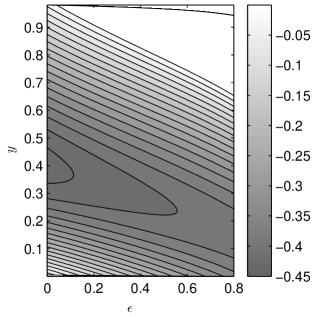
Since we perform here the perturbative calculation up to the 14th order, we expect that this calculation allows us also to obtain some information about the region of $y<1/3$. From the Fig. 4 (or more precisely from the numerical data), one can read off the optimal value of $\epsilon$, i.e. optimal value of $\Delta$. Solving the Bethe ansatz integral equation for this value of $\Delta$ we can recover in this way the full information about the corresponding optimal quantum state.

VIII Conclusions

In this paper we have studied the question posed by O’Connor and Wootters concerning translationally invariant states of $N$ qubits with maximal nearest neighbor (NN) concurrence. We have answered this question for $N\rightarrow\infty$ using the mapping of the problem onto the search for ground states of a certain family of “parent” Hamiltonians, described by the XXZ model. Using the analytic Bethe ansatz solutions of the XXZ model in the limit $N\to\infty$ (combining analytic results of low order perturbation theory and a numerical calculation of the 14th order perturbation theory) we have proved that: (i) for a given number of spins “down”, i.e. a given magnetization $y$ larger than $1/3$, the states that maximize the NN concurrence coincide with the ones obtained by O’Connor and Wootters, i.e. do not have NN pairs of spins “down”; (ii) For small magnetizations, more explicitly for $0\leq y\leq 1/3$, the states that maximize the NN concurrence do contain nearest neighbor pairs of spins “down”; (iii) in particular, the state that maximizes the NN concurrence without constraint on $y$ belongs to the family introduced by O’Connor and Wootters. Our results shed more light on the subtle relations between entanglement in spin 1/2 models and the ferromagnetic/anti-ferromagnetic character of spin-spin interactions. In the appendix we present some simple bounds on the optimal magnetic field that corresponds to the maximal NN concurrence.

We acknowledge the support of The Danish Natural Science Research Council, DFG (SFB 407, SPP 1078, SPP 1116), ESF Program “QUDEDIS”, EU FET IST 6th Framework Integrated Project “SCALA”, and Spanish MEC Grant FIS2005-04627.

Appendix A Bound on the optimal magnetic field

If one keeps $y$ fixed, and use $\mathcal{H}$ to parameterize the $s$-curve instead of $s$, one gets:

$$\frac{dE_{\mathrm{GS}}}{d\mathcal{H}} = -\frac{d\Delta}{d\mathcal{H}}\frac{1}{2}\left[1+\langle\sigma_{z}\sigma_{z}\rangle\right]-y$$

$$= 2\frac{\mathcal{H}}{\sqrt{\mathcal{H}^{2}+1}}P+\left(\frac{\mathcal{H}}{\sqrt{\mathcal{H}^{2}+1}}-1\right)y,$$

where $P$ is the probability of two neighboring spins being both “down”.

Demanding that $\frac{dE_{\mathrm{GS}}}{d\mathcal{H}}=0$, we find:

$$\mathcal{H}_{\mathrm{opt}}=\pm y/(2\sqrt{P}\sqrt{P+y})$$

where $\mathcal{H}_{\mathrm{opt}}$ is the optimal magnetic field. Obviously, $\mathcal{H}_{opt}=0$ iff $y=0$.

Using a simple bound on $P$,

$$P\leq(y+1)/2\quad\text{in the limit}\quad N\rightarrow\infty,$$

we obtain a lower bound on $\mathcal{H}_{\mathrm{opt}}$:

$$\mathcal{H}_{\mathrm{opt}}\geq y/(\sqrt{y+1}\sqrt{3y+1}).$$

This bound does not work well for $y>1/3$, because it gives a finite bound, maximized for $y=1$ when we find $\mathcal{H}_{\mathrm{opt}}\geq 1/(2\sqrt{2})$, whereas we know that in this regime of $y$’s $\mathcal{H}_{\mathrm{opt}}=\infty$. For smaller values of $y<1/3$, both the optimal $\epsilon$ (i.e. $\Delta$, see Fig. 4), as well as the optimal $\mathcal{H}_{\mathrm{opt}}$ attain finite values, so that the bound might become more useful. In particular, the results of Fig. 4 suggest that as $y$ approaches zero, the optimal $\epsilon$ approaches 1 more or less linearly, as $1-(1/3)^{-1}y$, which in turn implies that the optimal $\Delta$ approaches $-1$ as $-1-3y$. Thus for small $y$ and small $\Delta+1$, the bound becomes $\mathcal{H}_{\mathrm{opt}}\geq-\frac{1}{3}(1+\Delta)$, which already is not obvious (compare Fig. 1).

References

- (1) For the theory, see e.g. D. Jaksch, C. Bruder, J. I. Cirac, C. W. Gardiner, and P. Zoller, Phys. Rev. Lett. 81, 3108 (1998); D. Jaksch, H.-J. Briegel, J. I. Cirac, C. W. Gardiner, and P. Zoller, Phys. Rev. Lett. 82, 1975 (1999); J. K. Pachos and M. B. Plenio, Phys. Rev. Lett. 93, 056402 (2004); C. M. Alves and D. Jaksch, Phys. Rev. Lett. 93, 110501 (2004). For the experiments, see e.g. O. Mandel, M. Greiner, A. Widera, T. Rom, T. W. Hänsch and I. Bloch, Nature 425, 937 (2003).
- (2) L.-M. Duan, A. Sørensen, J. I. Cirac, and P. Zoller, Phys. Rev. Lett. 85, 3991 (2000); M. G. Moore and P. Meystre, Phys. Rev. Lett. 85, 5026 (2000).
- (3) A. Osterloh, L. Amico, G. Falci, and R. Fazio, Nature 416, 608 (2002).
- (4) T. J. Osborne and M. A. Nielsen, Phys. Rev. A 66, 032110 (2002).
- (5) G. Vidal, J. I. Latorre, E. Rico, and A. Kitaev, Phys. Rev. Lett. 90, 227902 (2003); J. I. Latorre, E. Rico, and G. Vidal, QIC 4, 48 (2004).
- (6) J. Vidal, R. Mosseri, and J. Dukelsky, Phys. Rev. A 69, 054101 (2004); L.-A. Wu, M. S. Sarandy, and D. A. Lidar, Phys. Rev. Lett. 93, 250404 (2004); L.-A. Wu, S. Bandyopadhyay, M. S. Sarandy, D. A. Lidar, Phys. Rev. A 72, 032309 (2005); M.-F. Yang, Phys. Rev. A 71, 030302(R) (2005).
- (7) I. Bose and E. Chattopadhyay, Phys. Rev. A 66, 062320 (2002); A. Hutton and S. Bose, Phys. Rev. A 69, 042312 (2004); A. Hutton and S. Bose, quant-ph/0408077; M. Wieśniak, V. Vedral, and Č. Brukner, New J. Phys. 7, 258 (2005); I. Bose and A. Tribedi, Phys. Rev. A 72, 022314 (2005); P. Calabrese and J. Cardy, J. Stat. Mech. P04010 (2005).
- (8) K. Audenaert, J. Eisert, M. B. Plenio, and R. F. Werner, Phys. Rev. A66, 042327 (2002).
- (9) U. V. Poulsen, T. Meyer, and M. Lewenstein, Phys. Rev. A71, 063605 (2005).
- (10) N. Schuch, J. I. Cirac, and M. M. Wolf, quant-ph/0509166; M. Cramer and J. Eisert, quant-ph/0509167.
- (11) L. Bombelli, R. K. Koul, J. Lee, and R. D. Sorkin, Phys. Rev. D 34, 373 (1986); M. Srednicki, Phys. Rev. Lett. 71, 666 (1993).
- (12) J. I. Latorre, R. Orus, E. Rico, J. Vidal, Phys. Rev. A 71, 064101 (2005); P. Calabrese and J. Cardy, J. Stat. Mech., P06002 (2004); A. R. Its, B.-Q. Jin, and V. E. Korepin, J. Phys. A: Math. Gen. 38, 2975 (2005); B.-Q. Jin and V. E. Korepin, J. Stat. Phys. 116, 79 (2004); J.P. Keating and F. Mezzadri, Phys. Rev. Lett. 94, 050501 (2005); M. B. Plenio, J. Eisert, J. Dreissig, and M. Cramer, Phys. Rev. Lett. 94 060503 (2005); M. Cramer, J. Eisert, M. B. Plenio, and J. Dreissig, Phys. Rev. A 73, 012309 (2006).
- (13) W. Dür, L. Hartmann, M. Hein, M. Lewenstein, and H.-J. Briegel, Phys. Rev. Lett. 94, 097203 (2005).
- (14) F. Verstraete, M. Popp, and J. I. Cirac, Phys. Rev. Lett. 92, 027901 (2004); F. Verstraete, M. A. Martin-Delgado, and J. I. Cirac, ibid., 087201 (2004).
- (15) M. Popp, F. Verstraete, M. A. Martin-Delgado, and J. I. Cirac, Phys. Rev. A 71, 042306 (2005).
- (16) D. Aharonov, Phys. Rev. A 62, 062311 (2000).
- (17) S. Popescu and D. Rohrlich, Phys. Lett. A 166, 293 (1992).
- (18) A. Sen(De), U. Sen, M. Wieśniak, D. Kaszlikowski, and M. Żukowski, Phys. Rev. A 68, 062306 (2003); A. Sen(De), U. Sen, and M Żukowski, Phys. Rev. A 68, 032309 (2003).
- (19) B.-Q. Jin and V. E. Korepin, Phys. Rev. A 69, 062314 2004.
- (20) D. P. DiVincenzo, C. A. Fuchs, H. Mabuchi, J. A. Smolin, A. Thapliyal, A. Uhlmann, quant-ph/9803033; O. Cohen, Phys. Rev. Lett. 80, 2493 (1998); T. Laustsen, F. Verstraete, and S. J. van Enk, QIC 3, 64 (2003).
- (21) D. Bruß, N. Datta, A. Ekert, L.C. Kwek, C. Macchiavello, Phys. Rev. A 72, 014301 (2005), O. Gühne, G. Toth, H.-J. Briegel, New J. Phys. 7, 229 (2005).
- (22) H.-J. Briegel and R. Raussendorf, Phys. Rev. Lett. 86, 910 (2001); R. Raussendorf and H.-J. Briegel, Phys. Rev. Lett. 86, 5188 (2001).
- (23) L. Amico, A. Osterloh, F. Plastina, R. Fazio, and G. M. Palma, Phys. Rev. A 69, 022304 (2004).
- (24) A. Sen(De), U. Sen, and M. Lewenstein, Phys. Rev. A 70, 060304(R) (2004).
- (25) S. Bose, Phys. Rev. Lett. 91, 207901 (2003).
- (26) C. H. Bennett, G. Brassard, C. Crépeau, R. Jozsa, A. Peres, and W. K. Wootters, Phys. Rev. Lett. 70, 1895 (1993).
- (27) R. Raussendorf, D. E. Browne, and H.-J. Briegel, Phys. Rev. A 68, 022312 (2003); M. A. Nielsen, Phys. Rev. Lett. 93, 040503 (2004); D. E. Browne and T. Rudolph, Phys. Rev. Lett. 95, 010501 (2005).
- (28) V. Subrahmanyam, Phys. Rev. A 69, 034304 (2004); M. Christandl, N. Datta, A. Ekert, and A. J. Landahl, Phys. Rev. Lett. 92, 187902 (2004); D. Burgarth and S. Bose, Phys. Rev. A 71, 052315 (2005); S. Bose, B.-Q. Jin, and V. E. Korepin, Phys. Rev. A 72, 022345 (2005); D. Burgarth, V. Giovannetti, and S. Bose, J. Phys. A: Math. Gen 38, 6793 (2005), and references therein.
- (29) A. Sen (De), U. Sen, and M. Lewenstein, Phys. Rev. A 72, 052319 (2005).
- (30) G. Vidal, Phys. Rev. Lett. 93, 040502 (2004); F. Verstraete, D. Porras, and J. I. Cirac, Phys. Rev. Lett. 93, 227205 (2004); F. Verstraete, J. J. Garcia-Ripoll, and J. I. Cirac, Phys. Rev. Lett. 93, 207204 (2004); M. Zwolak and G. Vidal, Phys. Rev. Lett. 93, 207205 (2004); F. Verstraete and J. I. Cirac, cond-mat/0407066; C. Kollath, U. Schollwöck, J. von Delft, and W. Zwerger, Phys. Rev. A71, 053606 (2005); for applications, see for instance S.R. Clark and D. Jaksch, Phys. Rev A 70, 043612 (2004), Phys. Rev. A70, 043612 (2004); A. J. Daley, S. R. Clark, D. Jaksch, and P. Zoller, Phys. Rev. A 72, 043618 (2005).
- (31) W. K. Wootters, Contemp. Math. 305, 299 (2002); K. M. O’Connor and W. K. Wootters, Phys. Rev. A, 63, 052302 (2001); W. K. Wootters, quant-ph/0202048.
- (32) D. Bruß, Phys. Rev. A 60, 4344 (1999).
- (33) V. Coffman, J. Kundu, and W. K. Wootters, Phys. Rev. A 61, 052306 (2000).
- (34) T. Meyer, U. V. Poulsen, K. Eckert, M. Lewenstein, D. Bruß, Int. J. Quant. Inf. 2, 149 (2004);
- (35) M. M. Wolf, F. Verstraete, and J. I. Cirac, Int. J. Quantum Inf. 1, 465 (2003).
- (36) W. K. Wootters, Phys. Rev. Lett. 80, 2245 (1998)
- (37) R. A. Horn and C. R. Johnson, Matrix Analysis, (Cambridge University Press, Cambridge, 1985), page 414.
- (38) C. N. Yang and C. P. Yang, Phys. Rev. 150, 321 (1966).
- (39) C. N. Yang and C. P. Yang, Phys. Rev. 150, 327 (1966).
- (40) C. N. Yang and C. P. Yang, Phys. Rev. 151, 258 (1966).
- (41) V. E. Korepin, N. M. Bogoliubov, and A. G.Izergin, Quantum Inverse Scattering Method and Correlation Functions, Cambridge Monographs on Mathematical Physics (Cambridge University Press, Cambridge, UK, 1993).
- (42) J. D. Johnson, J. Appl. Phys. 52, 1991, (1981).