Quantum-state input-output relations for absorbing cavities

Abstract

The quantized electromagnetic field inside and outside an absorbing high-$Q$ cavity is studied, with special emphasis on the absorption losses in the coupling mirror and their influence on the outgoing field. Generalized operator input-output relations are derived, which are used to calculate the Wigner function of the outgoing field. To illustrate the theory, the preparation of the outgoing field in a Schrödinger cat-like state is discussed.
Keywords: cavity QED, nonclassical states of the electromagnetic field, quantum state engineering, input-output relations

1 Introduction

Cavity QED provides a rich tool for experimental tests and applications of quantum mechanics, with special emphasis on quantum decoherence and communication [1]. The use of high-$Q$ cavities makes it possible to control the evolution of coupled atom-field systems in order to synthesize, at least on principle, arbitrary nonclassical states of light [2, 3, 4]. For example, schemes have been developed to generate various nonclassical states of light by mapping atomic Zeeman states on states of cavity fields [8, 9]. Nonclassical states of light on their part play a fundamental role in quantum information processing [5, 6, 7].

Unfortunately Nature imposes limits on us, because of quantum decoherence, which is unavoidably connected with the losses that are always present in practice. In cavities both wanted and unwanted losses play a role. Whereas the wanted losses, which result from the input-output coupling, typically affect the quantum state of the cavity field, unwanted losses such as scattering and absorption losses affect both the quantum state of the cavity field and the quantum state of the outgoing field. Keeping track of leaking emission renders possible for real-time measurement of the quantum state of the field and, therefore, offers the possibility of feedback control of open cavities [10], provided that the input-output coupling can be regarded as being the main source of decoherence. For high-$Q$ cavities this must not necessarily be the case. Moreover, when in quantum networks the radiation emitted by cavities plays the role of quantum communication channels connecting, e.g., atoms trapped in distantly separated cavities [11, 12], even small unwanted losses can lead to a noticeable degradation of the nonclassical features of the radiation [13].

In the rest of this article we study the problem of the absorption losses of a high-$Q$ cavity and their effect on the quantum state of the outgoing field in more detail, with special emphasis on the absorption losses in the coupling mirror. Basing the calculations on quantum electrodynamics in dispersing and absorbing media, we derive a formula that relates the Wigner function of the outgoing field to the Wigner functions of the cavity field, the incoming field, and the dissipative channels. As an application of the theory, we study a scheme for generating Schrödinger cat-like states by combining two incoming modes prepared in coherent states with a cavity mode prepared in a squeezed number state.

The paper is organized as follows. In section 2 the cavity model is described and the basic equations are given. Expressions for the cavity field and the outgoing field are given in sections 3 and 4, respectively. The Wigner function of the quantum state of the outgoing field is derived in section 5, and section 6 presents an application. Finally, the main results are summarized in section 7.

2 Cavity model

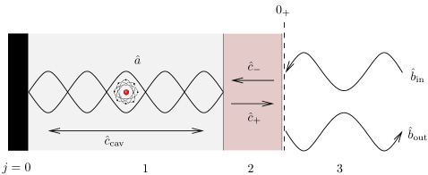
Figure 1: Scheme of the cavity. The fractionally transparent mirror (region (2)) is modelled by a dielectric plate. The active sources are in region 1, which can also contain some medium.

For simplicity let us consider a modified version of Ley and Loudon’s [14] cavity model, defined by a planar multi-layer system according to figure 1, where the layer labelled $j$ $\!=$ $\!0$ is assumed to be the totally reflecting mirror and the semitransparent mirror (layer $2$) is modelled by a dielectric plate. The linearly polarized electromagnetic waves propagate in the $z$ direction, for which we use shifted coordinate systems such that $0$ $\!<$ $\!z$ $\!<$ $\!l$ for $j$ $\!=$ $\!1$, $0$ $\!<$ $\!z$ $\!<$ $\!d$ for $j$ $\!=$ $\!2$, and $0$ $\!<$ $\!z$ $\!<\infty$ for $j$ $\!=$ $\!3$. Applying the one-dimensional version of the quantization scheme in reference [15, 16], allowing for active atomic sources inside the cavity [$A$th atom with electric dipole moment $\hat{d}_{A}(t)$ being at position $z_{A}$], and following reference [17], we may represent the electric field in the $j$th layer of permittivity $\varepsilon_{j}(\omega)$ ($j$ $\!=$ $\!1,2,3$) in the form of

$$\hat{E}^{(j)}(z,t)=\int_{0}^{\infty}\mbox{\rm d}\omega\,\underline{\hat{E}}{{}^{(j)}}(z,\omega,t)+\mathrm{H.c.},$$ (1)

$$\underline{\hat{E}}{{}^{(j)}}(z,\omega,t)=\underline{\hat{E}}^{(j)}_{\mathrm{free}}(z,\omega,t)+\underline{\hat{E}}^{(j)}_{\mathrm{s}}(z,\omega,t),$$ (2)

where

$$\underline{\hat{E}}^{(j)}_{\mathrm{free}}(z,\omega,t)=i\omega\mu_{0}\sum_{j^{\prime}=1}^{3}\int_{[j^{\prime}]}\mbox{\rm d}z^{\prime}\,G^{(jj^{\prime})}(z,z^{\prime},\omega)\hat{\underline{j}}^{(j^{\prime})}_{\mathrm{free}}(z^{\prime},\omega,t)$$ (3)

is the free-field part ($[j^{\prime}]$ indicates integration over the $j^{\prime}$th layer),

$$\underline{\hat{E}}^{(j)}_{\mathrm{s}}(z,\omega,t)=\frac{i}{\pi\epsilon_{0}\mathcal{A}}\,\frac{\omega^{2}}{c^{2}}\!\sum_{A}\!\int\!\mbox{\rm d}t^{\prime}\,\Theta(t-t^{\prime})e^{-i\omega(t-t^{\prime})}\hat{d}_{A}(t^{\prime})\,\mathrm{Im}\,G^{(1j)}(z_{A},z,\omega)$$ (4)

($\mathcal{A}$: mirror area) is the source-field part, and

$$\underline{\hat{j}}^{(j)}_{\mathrm{free}}(z,\omega,t)=\omega\,\sqrt{\frac{\hbar\epsilon_{0}}{\pi{\cal A}}\,\varepsilon^{\prime\prime}_{j}(\omega)}\,\hat{f}^{(j)}_{\mathrm{free}}(z,\omega,t)$$ (5)

[$\hat{f}^{(j)}_{\mathrm{free}}(z,\omega,t)$ $\!=$ $\!e^{-i\omega(t-t^{\prime})}\hat{f}^{(j)}_{\mathrm{free}}(z,\omega,t^{\prime})$; $\hat{f}^{(j)}(z,\omega,t)$, bosonic fields; $\varepsilon_{j}(\omega)$ $\!=$ $\!\varepsilon^{\prime}_{j}(\omega)$ $\!+$ $\!i\varepsilon_{j}^{\prime\prime}(\omega)$]. Further,

$$G^{(jj^{\prime})}(z,z^{\prime},\omega) = {\textstyle\frac{1}{2}}i\bigl{[}\mathcal{E}^{j>}(z,\omega)\,\Xi^{jj^{\prime}}\mathcal{E}^{j^{\prime}<}(z^{\prime},\omega)\Theta(j-j^{\prime})$$ (6)

$$+\mathcal{E}^{j<}(z,\omega)\,\Xi^{j^{\prime}j}\mathcal{E}^{j^{\prime}>}(z^{\prime},\omega)\Theta(j^{\prime}-j)\bigr{]}$$

is the (nonlocal part of the) Green function, where the functions

$$\mathcal{E}^{(j)>}(z,\omega)=e^{i\beta_{j}(z-d_{j})}+r_{j/3}e^{-i\beta_{j}(z-d_{j})}$$ (7)

and

$${\mathcal{E}}^{(j)<}(z,\omega)\,=\,e^{-i\beta_{j}z}+r_{j/0}e^{i\beta_{j}z}$$ (8)

represent waves of unit strength travelling, respectively, rightward and leftward in the $j$th layer and being reflected at the boundary [note that $\Theta(j$ $\!-$ $\!j^{\prime})$ means $\Theta(z$ $\!-$ $\!z^{\prime})$ for $j$ $\!=$ $\!j^{\prime}$]. Further, $\Xi^{jj^{\prime}}$ is defined by

$$\Xi^{jj^{\prime}}=\frac{1}{\beta_{3}t_{0/3}}\,\frac{t_{0/j}e^{i\beta_{j}d_{j}}}{D_{j}}\,\frac{t_{3/j^{\prime}}e^{i\beta_{j^{\prime}}d_{j^{\prime}}}}{D_{j^{\prime}}}\,,$$ (9)

where

$$D_{j}=1-r_{j/0}r_{j/3}e^{2i\beta_{j}d_{j}}$$ (10)

and

$$\beta_{j}\equiv\beta_{j}(\omega)=\sqrt{\varepsilon_{j}(\omega)}\,\frac{\omega}{c}=\left[n_{j}^{\prime}(\omega)+in_{j}^{\prime\prime}(\omega)\right]\,\frac{\omega}{c}=\beta_{j}^{\prime}+i\beta_{j}^{\prime\prime}$$ (11)

[$\beta_{j}^{\prime},\beta_{j}^{\prime\prime}$ $\!\geq$ $\!0$, $d_{1}$ $\!=$ $\!l$, $d_{2}$ $\!=$ $\!d$, $d_{3}$ $\!=$ $\!0$]. The quantities $t_{j/j^{\prime}}$ $\!=$ $\!(\beta_{j}/\beta_{j^{\prime}})t_{j^{\prime}/j}$ and $r_{j/j^{\prime}}$ are respectively the transmission and reflection coefficients between the layers $j^{\prime}$ and $j$, which can be recursively determined. Note, for the cavity model under consideration $r_{10}$ $\!=$ $\!-1$, since perfect reflection from the left-side mirror has been assumed.

3 Cavity field

To evaluate, according to equations (1)–(4) for $j$ $\!=$ $\!1$, the electric field inside the cavity, we notice that the function $D_{1}(\omega)$ given by equation (10) defines the spectral response of the cavity. That is, the complex resonance frequencies $\Omega_{k}$ $\!=$ $\!\omega_{k}$ $\!-$ $\!{\textstyle\frac{1}{2}}i\Gamma_{k}$ of the cavity field are determined by the zeroes of

$$D_{1}(\Omega_{k})=1+r_{13}(\Omega_{k})e^{2i\beta_{1}(\Omega_{k})l}=0$$ (12)

and may be found by iteration. Somewhat lengthy but straightforward calculations show that – provided that $\Gamma_{k}$ $\!\ll$ $\!\Delta\omega_{k}$, with $\Delta\omega_{k}$ $\!=$ $\!\frac{1}{2}(\omega_{k+1}$ $\!-$ $\!\omega_{k-1})$ being the width of the $k$th interval – equation (1) [together with equations (2)–(4)] can be approximately rewritten as

$$\hat{E}^{(1)}(z,t)=\sum_{k}E_{k}(z)\hat{a}_{k}(t)+\mathrm{H.c.},$$ (13)

where the standing wave mode functions are defined as

$$E_{k}(z)=i\omega_{k}\left[\frac{\hbar}{\epsilon_{0}\varepsilon_{1}(\omega_{k})l{\cal A}\omega_{k}}\right]^{\frac{1}{2}}\sin[\beta_{1}(\omega_{k})z],$$ (14)

and

$$\hat{a}_{k}(t)=\int\mbox{\rm d}t^{\prime}\,\Theta(t-t^{\prime})e^{-i\Omega_{k}(t-t^{\prime})}$$

$$\hskip 8.61108pt\times\biggl{\{}\biggl{[}\frac{c}{2n_{1}(\omega_{k})l}\biggr{]}^{\frac{1}{2}}\biggl{[}T_{k}\hat{b}_{k\mathrm{in}}(t^{\prime})+\sum_{\lambda}A_{k{\lambda}}\hat{c}_{k{\lambda}}(t^{\prime})\biggr{]}-\frac{i}{\hbar}\sum_{A}E_{k}(z_{A})\hat{d}_{A}(t^{\prime})\biggr{\}}.$$ (15)

Here the operators $\hat{c}_{k\lambda}(t)$ and $\hat{b}_{k\mathrm{in}}(t)$ are defined by

$$\hat{c}_{k\lambda}(t)=\frac{1}{\sqrt{2\pi}}\int_{(\Delta_{k})}\mbox{\rm d}\omega\,\hat{c}_{\lambda}(\omega,t),$$ (16)

$$\hat{b}_{k\mathrm{in}}(t)=\frac{1}{\sqrt{2\pi}}\int_{(\Delta_{k})}\mbox{\rm d}\omega\,\hat{b}_{\mathrm{in}}(\omega,t),$$ (17)

where the integration runs in the interval $(\Delta_{k})$ $\!\equiv$ $[\frac{1}{2}(\omega_{k-1}$ $\!+$ $\!\omega_{k}),\frac{1}{2}(\omega_{k}$ $\!+$ $\!\omega_{k+1})]$, and the bosonic operators $\hat{b}_{\mathrm{in}}(\omega,t)$ and $\hat{c}_{\lambda}(\omega,t)$ ($\lambda$ $\!=$ $\!\mathrm{cav},\pm$) read

$$\hat{b}_{\mathrm{in}}(\omega,t)=-\sqrt{\frac{\mu_{0}c\pi\mathcal{A}}{\hbar\omega}}\frac{|n_{3}|}{n_{3}\sqrt{n_{3}^{\prime}}}\int_{[3]}\mbox{\rm d}z^{\prime}\,e^{i\beta_{3}z^{\prime}}\underline{\hat{j}}^{(3)}_{\mathrm{free}}(z^{\prime},\omega,t),$$ (18)

$$\hat{c}_{\pm}(\omega,t)=-\alpha_{\pm}\sqrt{\frac{\mu_{0}c\pi\mathcal{A}}{\hbar\omega}}\frac{1}{2n_{2}}\int_{[2]}\mbox{\rm d}z^{\prime}\,\left[e^{-i\beta_{2}(z^{\prime}-d)}\pm e^{i\beta_{2}z^{\prime}}\right]\underline{\hat{j}}^{(2)}_{\mathrm{free}}(z^{\prime},\omega,t),$$ (19)

$$\hat{c}_{\mathrm{cav}}(\omega,t)=-\alpha_{\mathrm{cav}}\sqrt{\frac{\mu_{0}c\pi\mathcal{A}}{\hbar\omega}}\frac{1}{2n_{1}}\int_{[1]}\mbox{\rm d}z\,\sin(\beta_{1}z)\underline{\hat{j}}^{(1)}_{\mathrm{free}}(z,\omega,t),$$ (20)

with

$$\alpha_{\mathrm{cav}}=\alpha_{\mathrm{cav}}(\omega)=2\sqrt{2}|n_{1}|\left[n_{1}^{\prime}\sinh(2\beta_{1}^{\prime\prime}l)-n_{1}^{\prime\prime}\sin(2\beta_{1}^{\prime}l)\right]^{-\frac{1}{2}},$$ (21)

$$\alpha_{\pm}=\alpha_{\pm}(\omega)=|n_{2}|e^{\beta_{2}^{\prime\prime}d/2}\left[n_{2}^{\prime}\sinh(\beta_{2}^{\prime\prime}d)\pm n_{2}^{\prime\prime}\sin(\beta_{2}^{\prime}d)\right]^{-\frac{1}{2}},$$ (22)

and the coefficients $T_{k}$, $A_{k\lambda}$ are defined according to

$$T_{k}=T(\omega_{k}), T(\omega)=-\frac{t_{31}\sqrt{n_{1}n_{3}^{\prime}}}{|n_{3}|}\,e^{i\beta_{1}l},$$ (23)

$$A_{k\pm}=A_{\pm}(\omega_{k}), A_{\pm}(\omega)=-\frac{t_{21}\sqrt{n_{1}}}{D_{2}^{\prime}\alpha_{\pm}}\left(r_{23}e^{i\beta_{2}d}\pm 1\right)e^{i\beta_{1}l},$$ (24)

$$A_{k\mathrm{cav}}=A_{\mathrm{cav}}(\omega_{k}), A_{\mathrm{cav}}(\omega)=-4i\,\frac{\sqrt{n_{1}}}{\alpha_{\mathrm{cav}}}\,.$$ (25)

It can be proved that the operators $\hat{b}_{k\mathrm{in}}(t)$ and $\hat{c}_{k\lambda}(t)$ satisfy, on a (course-grained) timescale $\Delta t$ $\!\gg$ $\Delta\omega_{k}^{-1},\Delta\omega_{k^{\prime}}^{-1}$, the commutation relations

$$\bigl{[}\hat{b}_{k\mathrm{in}}(t),\hat{b}_{k^{\prime}\mathrm{in}}^{\dagger}(t^{\prime})\bigr{]}=\delta_{kk^{\prime}}\delta(t-t^{\prime}),$$ (26)

$$\bigl{[}\hat{c}_{k\lambda}(t),\hat{c}_{k^{\prime}\lambda^{\prime}}^{\dagger}(t^{\prime})\bigr{]}=\delta_{kk^{\prime}}\delta_{\lambda\lambda^{\prime}}\delta(t-t^{\prime}),$$ (27)

and the equal-time commutation relation

$$[\hat{a}_{k}(t),\hat{a}_{k^{\prime}}^{\dagger}(t)]=\delta_{kk^{\prime}}$$ (28)

hold. From equation (3) it follows that $\hat{a}_{k}(t)$ obeys the Langevin equation

$$\dot{\hat{a}}_{k} = -i\left(\omega_{k}-{\textstyle\frac{1}{2}}i\Gamma_{k}\right)\hat{a}_{k}-\frac{i}{\hbar}\sum_{A}E_{k}(z_{A})\hat{d}_{A}$$ (29)

$$+\biggl{[}\frac{c}{2n_{1}(\omega_{k})l}\biggr{]}^{\frac{1}{2}}\biggl{[}T_{k}\hat{b}_{k\mathrm{in}}(t)+\sum_{\lambda}A_{k\lambda}\hat{c}_{k\lambda}(t)\biggr{]}.$$

Within the approximation scheme used, the total decay rate $\Gamma_{k}$ determined from equation (12) can be decomposed into a radiative part $\gamma_{k\mathrm{rad}}$ and a non-radiative part $\gamma_{k\mathrm{abs}}$,

$$\Gamma_{k}=\gamma_{k\mathrm{rad}}+\gamma_{k\mathrm{abs}},$$ (30)

where

$$\gamma_{k\mathrm{rad}}=\frac{c}{2|n_{1}(\omega_{k})|l}|T_{k}|^{2},$$ (31)

$$\gamma_{k\mathrm{abs}}=\sum_{\lambda}\gamma_{k\lambda}=\frac{c}{2|n_{1}(\omega_{k})|l}\sum_{\lambda}|A_{k\lambda}|^{2}.$$ (32)

Note, that Langevin equations of the type of equation (29) can be also obtained from quantum noise theories on the basis of an appropriately chosen Senitzky-Gardiner-Collett Hamiltonian [18, 19].

4 Input-output relations

For simplicity we restrict ourselves to the case of a cavity in free space, i.e., $n_{3}\to 1$. To determine the input-output relations, we decompose the field outside the cavity [equations(1)–(4) for $j$ $\!=$ $\!3$ together with the Green function (6)] into incoming and outgoing parts and introduce the bosonic operators

$$\hat{b}_{\mathrm{out}}(\omega,t)=2\sqrt{\frac{\pi\mathcal{A}}{\mu_{0}c\hbar\omega}}\,\underline{\hat{E}}^{(3)}_{\mathrm{out}}(z,\omega,t)\bigr{|}_{z=0^{+}}.$$ (33)

Recalling the resonance structure of the spectral response of the cavity, we may write

$$\hat{b}_{\mathrm{out}}(t)=\frac{1}{\sqrt{2\pi}}\int\mathrm{d}\omega\,\hat{b}_{\mathrm{out}}(\omega,t)=\sum_{k}\hat{b}_{k\mathrm{out}}(t),$$ (34)

$$\hat{b}_{k\mathrm{out}}(t)=\frac{1}{\sqrt{2\pi}}\int_{(\Delta_{k})}\mathrm{d}\omega\,\hat{b}_{k\mathrm{out}}(\omega,t),$$ (35)

where, within the approximation scheme used,

$$\hat{b}_{k\mathrm{out}}(\omega,t)=\sqrt{\frac{\pi\mathcal{A}}{\mu_{0}c\hbar\omega}}\frac{\omega_{k}t_{13}\exp[i\beta_{1}(\Omega_{k})l]}{\epsilon_{0}\varepsilon_{1}\!(\Omega_{k})l\mathcal{A}}$$

$$\times\,\sum_{A}\int\!\mbox{\rm d}t^{\prime}\Theta(t\!-\!t^{\prime})e^{-i\Omega_{k}(t-t^{\prime})}\hat{d}_{A}(t^{\prime})\sin[\beta_{1}\!(\Omega_{k})z_{A}]$$

$$+\frac{c}{2n_{1}l}\,T^{({\rm o})}(\omega)\int\mbox{\rm d}t^{\prime}\,\Theta(t-t^{\prime})e^{-i\Omega_{k}(t-t^{\prime})}\biggl{[}T(\omega)\hat{b}_{\mathrm{in}}(\omega,t^{\prime})+\sum_{\lambda}A_{\lambda}(\omega)\hat{c}_{\lambda}\!(\omega,t^{\prime})\biggr{]}$$

$$+A_{+}^{({\rm o})}(\omega)\hat{c}_{+}(\omega,t)+A_{-}^{({\rm o})}(\omega)\hat{c}_{-}(\omega,t)+R^{({\rm o})}(\omega)\hat{b}_{\mathrm{in}}(\omega,t),$$ (36)

with

$$A_{\pm}^{({\rm o})}(\omega)=\frac{t_{23}}{D_{2}^{\prime}}\frac{1\pm r_{21}e^{i\beta_{2}d}}{\alpha_{\pm}}\,,$$ (37)

$$T^{({\rm o})}(\omega)=\frac{t_{13}}{\sqrt{n_{1}}}\,e^{i\beta_{1}l},$$ (38)

$$R^{({\rm o})}(\omega)=r_{31}.$$ (39)

Performing in equation (35) the $\omega$ integration and recalling equations (3), (16), and (17), we obtain the generalized input-output relations

$$\hat{b}_{k\mathrm{out}}(t)=\left[\frac{c}{2n_{1}(\omega_{k})l}\right]^{\frac{1}{2}}\!T_{k}^{({\rm o})}\hat{a}_{k}(t)\!+\!R_{k}^{({\rm o})}\hat{b}_{k\mathrm{in}}(t)\!+\!A_{k+}^{({\rm o})}\hat{c}_{k+}(t)\!+\!A_{k-}^{({\rm o})}\hat{c}_{k-}(t)$$ (40)

[$T_{k}^{({\rm o})}$ $\!=$ $\!T^{({\rm o})}(\omega_{k})$, $A^{({\rm o})}_{k\pm}$ $\!=$ $\!A^{({\rm o})}_{\pm}(\omega_{k})$, $R_{k}^{({\rm o})}$ $\!=$ $\!R^{({\rm o})}(\omega_{k})$]. In close analogy to equation (26), the commutation relation

$$\bigl{[}\hat{b}_{k{\rm out}}(t),\hat{b}^{\dagger}_{k^{\prime}{\rm out}}(t^{\prime})\bigr{]}=\delta_{kk^{\prime}}\delta(t-t^{\prime})$$ (41)

can be shown to hold. Omitting the last two terms on the right-hand side in equation (40), which describe the effect on the outgoing field of the noise associated with the losses in the coupling mirror, we recover the input-output relations suggested by standard quantum noise theories [19]. Note, that a Hamiltonian of the Senitzky-Gardiner-Collett type [18, 19] is not suited for consideration of the effect.

5 Quantum-state extraction

Let us suppose that at some initial time $t_{0}$ the $k$th cavity mode is prepared in a certain quantum state and evolves freely for $t$ $\!\geq$ $t_{0}$ (the preparation time is assumed to be short compared to the decay time $\Gamma_{k}^{-1}$ of the cavity mode). From equations (29), (4), and (40) it then follows that

$$\hat{b}_{k\mathrm{out}}(\omega,t)=F^{*}_{k}(\omega,t)\hat{a}_{k}(t_{0})+\hat{B}_{k}(\omega,t),$$ (42)

where

$$F_{k}(\omega,t)=\frac{i}{\sqrt{2\pi}}\left(\frac{c}{2n_{1}^{*}l}\right)^{1/2}\!T_{k}^{({\rm o})*}f_{k}(\omega,t),$$ (43)

$$\hat{B}_{k}(\omega,t)\!=\!\!\int_{(\Delta_{k})}\!\mbox{\rm d}\omega^{\prime}\Bigl{[}G_{k\rm{in}}^{*}(\omega,\omega^{\prime},t)\hat{b}_{k\mathrm{in}}(\omega^{\prime},t_{0})\!+\!\sum_{\lambda}G_{k\lambda}^{*}(\omega,\omega^{\prime},t)\hat{c}_{k\lambda}(\omega^{\prime},t_{0})\Bigr{]},$$ (44)

with

$$f_{k}(\omega,t)=\frac{\exp\left[-i(\omega-\Omega^{*}_{k})(t+\Delta t-t_{0})\right]-1}{\omega-\Omega^{*}_{k}}\,e^{i\omega(t-t_{0})},$$ (45)

$$\upsilon(\omega,\omega^{\prime},t)=\frac{1}{2\pi}\frac{c}{2n_{1}^{*}l}\frac{1}{\omega-\omega^{\prime}}[f(\omega,t)-f(\omega^{\prime},t)e^{i(\omega^{\prime}-\omega)\Delta t}],$$ (46)

$$G_{k\rm{in}}(\omega,\omega^{\prime},t) =T_{k}^{({\rm o})*}T_{k}^{*}\upsilon_{k}(\omega,\omega^{\prime},t)+R_{k}^{({\rm o})*}e^{i\omega^{\prime}(t-t_{0})}\delta(\omega-\omega^{\prime}),$$ (47)

$$G_{k\rm{cav}}(\omega,\omega^{\prime},t) =T_{k}^{({\rm o})*}A_{k\mathrm{cav}}^{*}\upsilon_{k}(\omega,\omega^{\prime},t),$$ (48)

$$G_{k\pm}(\omega,\omega^{\prime},t) =T_{k}^{({\rm o})*}A^{*}_{k\pm}\upsilon_{k}(\omega,\omega^{\prime},t)+A^{({\rm o})*}_{k\pm}e^{i\omega^{\prime}(t-t_{0})}\delta(\omega-\omega^{\prime}).$$ (49)

For the following it will be convenient to introduce unitary, explicitly time-dependent transformations according to

$$\hat{b}_{k\mathrm{out}}(\omega,t) =\sum_{i}\phi_{\mathrm{out}}^{(i)*}(\omega,t)\hat{b}_{k\mathrm{out}}^{(i)}(t),$$ (50)

$$\hat{b}_{k\mathrm{in}}(\omega,t_{0}) =\sum_{i}\phi_{\mathrm{in}}^{(i)*}(\omega,t_{0})\hat{b}_{k\mathrm{in}}^{(i)}(t_{0}),$$ (51)

$$\hat{c}_{k\lambda}(\omega,t_{0}) =\sum_{i}\phi_{\lambda}^{(i)*}(\omega,t_{0})\hat{c}_{k\lambda}^{(i)}(t_{0}),$$ (52)

where, for chosen $t$ and $\varsigma$ ($\varsigma$ $\!=$ $\!\mathrm{out},\mathrm{in},\lambda$), the functions $\phi_{\varsigma}^{(i)}(\omega,t)$ are complete sets of square integrable orthonormal functions. Needless to say, that the bosonic commutation relations are preserved.

From equation (42) it is easy to see, that the cavity mode predominantly escapes into the outgoing mode with

$$\phi_{\mathrm{out}}^{(1)}(\omega,t)=\frac{F_{k}(\omega,t)}{\eta_{k}(t)}\,,$$ (53)

where

$$\eta_{k}(t)=\left[\int_{(\Delta_{k})}\mbox{\rm d}\omega\,|F_{k}(\omega,t)|^{2}\right]^{1/2}.$$ (54)

Hence, for chosen $k$, equation (42) takes the form

$$\hat{b}_{k\mathrm{out}}^{(i)}(t)=\left\{\begin{array}[]{ll}\eta_{k}(t)\,\hat{a}_{k}(t_{0})+\hat{B}_{k}^{(i)}(t)&\ \mathrm{if}\ i=1,\\[4.30554pt] \hat{B}_{k}^{(i)}(t)&\ \mathrm{otherwise},\end{array}\right.$$ (55)

where

$$\hat{B}_{k}^{(i)}(t)=\int_{(\Delta_{k})}\mbox{\rm d}\omega\,\phi_{\mathrm{out}}^{(i)}(\omega,t)\hat{B}_{k}(\omega,t),$$ (56)

and it can be proved that the commutation relations

$$\bigl{[}\hat{a}_{k}(t_{0}),\hat{B}_{k}^{(1)\dagger}(t)\bigr{]}=0\qquad(t\geq t_{0}),$$ (57)

$$\bigl{[}\hat{B}_{k}^{(1)}(t),\hat{B}_{k}^{(1)\dagger}(t)\bigr{]}=1-\eta_{k}^{2}(t)$$ (58)

hold.

It is now straightforward to calculate the characteristic function $C^{(1)}_{k{\rm out}}(\beta,t)$ of the quantum state of the relevant outgoing mode; for details, see reference [20]. The result reads [$\sigma$ $\!=$ $\!(\mathrm{in},\lambda)$]

$$C^{(1)}_{k{\rm out}}(\beta,t) = \exp\biggl{[}-{\textstyle\frac{1}{2}}|\beta|^{2}[1-\eta^{2}(t)-\sum_{\sigma,i}|\chi^{(i)}_{k\sigma}(t)|^{2}]\biggr{]}$$ (59)

$$\times\,C_{k}[\eta_{k}(t)\beta]\prod_{\sigma i}C^{(i)}_{k\sigma}[\chi^{(i)}_{k\sigma}(t)\beta],$$

where the mode couplings are defined as

$$\chi^{(i)}_{k\sigma}(t)=\int_{(\Delta_{k})}\mbox{\rm d}\omega\,\int_{(\Delta_{k})}\mbox{\rm d}\omega^{\prime}\,G_{k\sigma}(\omega,\omega^{\prime},t)\phi_{\mathrm{out}}^{(1)*}(\omega,t)\phi_{\sigma}^{(i)}(\omega^{\prime},t_{0}),$$ (60)

$C_{k}(\beta)$ is the characteristic function of the initially prepared quantum state of the cavity mode, and $C^{(i)}_{k\sigma}(\beta)$ are the characteristic functions of the modes of the incoming field ($\sigma$ $\!=$ $\!\mathrm{in}$) and the dissipative channels ($\sigma$ $\!=$ $\!\lambda$). From equation (59) the corresponding relation between the Wigner functions is derived to be [$\eta(t)$ $\!\equiv$ $\!\eta_{k}(t)$, $\chi_{\sigma}^{(i)}(t)$ $\!\equiv$ $\!\chi^{(i)}_{k\sigma}(t)$]

$$W_{{\rm out}}(\alpha,t)=\frac{2}{\pi}\frac{1}{1-\eta^{2}(t)-\sum_{\sigma i}|\chi_{\sigma}^{(i)}(t)|^{2}}$$

$$\hskip 17.22217pt\times\,\int\mbox{\rm d}^{2}\alpha^{\prime}\,W(\alpha^{\prime})\prod_{\sigma i}\int\mbox{\rm d}^{2}\alpha_{\sigma i}\,W_{\sigma}^{(i)}(\alpha_{\sigma i})\exp\!\left[-\frac{2|\eta(t)\,\alpha^{\prime}+\sum_{\sigma i}\chi_{\sigma}^{(i)}(t)\,\alpha_{\sigma i}-\alpha|^{2}}{1-\eta^{2}(t)-\sum_{\sigma i}|\chi_{\sigma}^{(i)}(t)|^{2}}\right],$$ (61)

where ($\gamma_{\mathrm{rad}}$ $\!\equiv$ $\!\gamma_{k\mathrm{rad}}$, $\gamma_{\mathrm{abs}}$ $\!\equiv$ $\!\gamma_{k\mathrm{abs}}$)

$$\eta^{2}(t)=\frac{\gamma_{\mathrm{rad}}^{({\rm o})}}{\gamma_{\mathrm{rad}}+\gamma_{\mathrm{abs}}}\left[1-e^{-(\gamma_{\mathrm{rad}}+\gamma_{\mathrm{abs}})(t+\Delta t-t_{0})}\right],$$ (62)

with

$$\gamma_{\mathrm{rad}}^{({\rm o})}=\gamma_{k\mathrm{rad}}^{({\rm o})}=\frac{c}{2|n_{1}|l}|T^{({\rm o})}_{k}|^{2}.$$ (63)

In particular, when the incoming modes and the dissipative channels are in thermal states (with average number of thermal photons $\bar{n}_{\sigma i}$), equation (5) reduces to

$$W_{{\rm out}}(\alpha,t)=\frac{2}{\pi}\frac{1}{1-\eta^{2}(t)+2\sum_{\sigma i}\bar{n}_{\sigma i}|\chi_{\sigma}^{(i)}(t)|^{2}}$$

$$\times\,\int\mbox{\rm d}^{2}\alpha^{\prime}\,\exp\!\left[\!-\frac{2|\eta(t)\,\alpha^{\prime}-\alpha|^{2}}{1-\eta^{2}(t)+2\sum_{\sigma i}\!\bar{n}_{\sigma i}|\chi_{\sigma}^{(i)}(t)|^{2}}\right]\!W(\alpha^{\prime}),$$ (64)

which reveals that the condition

$$\frac{\eta^{2}(t)}{1-\eta^{2}(t)+2\sum_{\sigma i}\bar{n}_{\sigma i}|\chi_{\sigma}^{(i)}(t)|^{2}}\gg 1$$ (65)

must be satisfied to ensure that the quantum state of the outgoing field becomes sufficiently close to the quantum state that the cavity field was initially prepared in. It should be pointed out that the additional noise terms in the input-output relation (40), which are associated with the losses in the coupling mirror, modify the functions $G_{k\sigma}(\omega,\omega^{\prime},t)$ [equations (47)–(49)], which leads, compared to standard noise theory, to an increased value of $2\sum_{\sigma i}\bar{n}_{\sigma i}|\chi_{\sigma}^{(i)}(t)|^{2}$ in equation (5), with the result that the condition of almost perfect quantum state extraction becomes more restrictive.

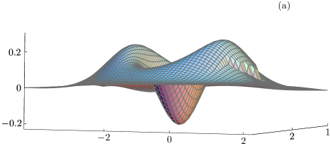
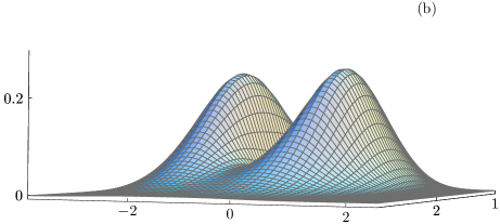
Figure 2: Wigner function of the output state for $n=1$, $r=0.8$, $\bar{n}=0.001$, $\beta=2$, (a) $\chi=0.1$, $\chi_{\mathrm{in}}=0.9$, $\eta=0.9$, (b) $\chi=0.7$, $\chi_{\mathrm{in}}=0.7$, $\eta=0.7$.

6 Generation of Schrödinger cat-like states

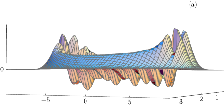
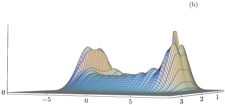
Figure 3: Wigner function of the output state for $n=10$, $r=1.1$, $\bar{n}=0.001$, $\beta=2$, (a) $\chi=0.1$, $\chi_{\mathrm{in}}=0.9$, $\eta=0.9$, (b) $\chi=0.7$, $\chi_{\mathrm{in}}=0.7$, $\eta=0.7$.

As an application of the theory, let us consider the case where two incoming modes with $\chi^{(1)}_{\mathrm{in}}(t)$ $\!=$ $\!\chi^{(2)}_{\mathrm{in}}(t)\equiv\chi_{\mathrm{in}}(t)$ are initially prepared in coherent states $\left|\beta\right\rangle$ and $\left|-i\beta\right\rangle$, respectively, and all other input modes and the dissipative channels are in thermal states with average numbers of thermal quanta $\bar{n}$. Then, from equation (5) we find

$$W_{{\rm out}}(\alpha,t)=\frac{2}{\pi}\frac{1}{1-\eta^{2}(t)+2\bar{n}|\chi(t)|^{2}}$$

$$\hskip 8.61108pt\times\,\int\mbox{\rm d}^{2}\alpha^{\prime}\,\exp\!\left[\!-\frac{2|\eta(t)\,\alpha^{\prime}-\alpha|^{2}}{1-\eta^{2}(t)+2\bar{n}|\chi(t)|^{2}}\right]\!W\Biggl{[}\alpha^{\prime}-\frac{\beta\chi_{\mathrm{in}}^{(1)}(t)}{\eta(t)}(1-i)\Biggr{]},$$ (66)

where the notation

$${\sum_{\sigma i}}^{\prime}\bar{n}|\chi_{\sigma}^{(j)}(t)|^{2}=\bar{n}|\chi(t)|^{2}$$ (67)

has been introduced, with the two incoming modes being excluded in the primed sum. Let us suppose that the cavity mode is initially prepared in a squeezed number state $|r,n\rangle$ $\!=$ $\!\hat{S}(r)|n\rangle$ [$\hat{S}(r)$, squeeze operator]. Examples of the Wigner function of the quantum state of the outgoing mode are plotted in figures 2 and 3 for $r=0.8$, $n=1$ and $r=1.1$, $n=10$, respectively, with $\bar{n}=0.001$, $\beta=2$ for both cases. As we can see from figures 2(a) and 3(a), the quantum state of the outgoing mode exhibits the typical features of a Schrödinger cat-like state, provided that the mode coupling is strong enough ($\chi_{\mathrm{in}}\to 1$) and the noise associated with the losses is sufficiently small ($\eta\to 1$, $\chi\to 0$). Figures 2(b) and 3(b) reveal, that with decreasing strength of the mode coupling and/or increasing noise the nonclassical features of the quantum state of the outgoing mode are completely lost. For the parameters chosen the nonclassical oscillatory fringes typical for a Schrödinger cat-like state can be observed as long as $\eta(t)$ $\!\geq$ $\!0.7$, which for $t$ $\!\to$ $\!\infty$ corresponds to the requirement that $\gamma_{\mathrm{abs}}$ $\lesssim$ $\gamma_{\mathrm{rad}}$. Note that the additional noise terms in the input-output relation (40), which are associated with the losses in the coupling mirror, effectively reduce the strength of the mode coupling $\chi_{\mathrm{in}}$. However, the necessary mode analysis will be considered in detail in a forthcoming paper.

7 Summary

To summarize, we have studied the input-output problem for a high-$Q$ cavity, with special emphasis on used input channels, taking into account the absorption losses in the coupling mirror. Within the framework of exact quantization of the electromagnetic field in dispersing and absorbing media we have performed the calculations for a one-dimensional cavity bounded by a perfectly reflecting mirror and a semi-transparent mirror. The theory generalizes the standard quantum noise theory based on a Hamiltonian of Senitzky-Gardiner-Collett type [18, 19], which does not fully take into account the absorption losses in the coupling mirror. Using the generalized operator input-output relations, we have calculated input-output relations for the Wigner functions of the quantum states involved. Finally, we have applied the theory to the case where two incoming modes prepared in coherent states are combined with a cavity mode initially prepared in a squeezed number state to prepare the outgoing field in a Schrödinger cat-like state.

References

References

• [1] Berman P R, Ed., 1994 Cavity Quantum Electrodynamics (Academic Press, San Diego, CA)
• [2] Brattke S, Varcoe B T H and Walther H 2001 Phys. Rev. Lett. 86 3534
• [3] Kuhn A, Hennrich M and Rempe G 2002 Phys. Rev. Lett. 89 067901
• [4] Raimond J M, Brune M and Haroche S 2001 Rev. Mod. Phys. 73 565
• [5] Monroe C 2002 Nature 416 238
• [6] Knill E, Laflamme R and Milburn G J 2001 Nature 409 461
• [7] Pellizzari T, Gardiner S A, Cirac J I and Zoller P 1995 Phys. Rev. Lett. 75 3788
• [8] Lange W and Kimble H J 2000 Phys. Rev. A 63 013401
• [9] Parkins A S, Marte P, Zoller P, Carnal O and Kimble H J 1995 Phys. Rev. A 51 1578
• [10] Doherty A C, Habib S, Jacobs K, Mabuchi H and Tan S M 2000 Phys. Rev. A 62 012105
• [11] Cirac J I, Zoller P, Kimble H J and Mabuchi H 1997 Phys. Rev. Lett. 78 3221
• [12] Browne D E, Plenio M B and Huelga S F 2003 Phys. Rev. Lett. 91 067901
• [13] Scheel S and Welsch D-G 2001 Phys. Rev. A 64 063811
• [14] Ley M and Loudon R 1987 J. Mod. Opt. 34 227
• [15] Scheel S, Knöll L and Welsch D-G 1998 Phys. Rev. A 58 700
• [16] Ho Trung Dung, Knöll L and Welsch D-G 2000 Phys. Rev. A 62 053804
• [17] Khanbekyan M, Knöll L and Welsch D-G 2003 Phys. Rev. A 67 063812
• [18] Senitzky I R 1959 Phys. Rev. 115 227
• [19] Collett M J and Gardiner C W 1984 Phys. Rev. A 30 1386
• [20] Khanbekyan M, Knöll L, Semenov A A, Vogel W and Welsch D-G 2004 Phys. Rev. A 69 043807