Dynamics of a pulsed continuous variable quantum memory

Abstract

We study the transfer dynamics of non-classical fluctuations of light to the ground-state collective spin components of an atomic ensemble during a pulsed quantum memory sequence, and evaluate the relevant physical quantities to be measured in order to characterize such a quantum memory. We show in particular that the fluctuations stored into the atoms are emitted in temporal modes which are always different than those of the readout pulse, but which can nevertheless be retrieved efficiently using a suitable temporal mode-matching technique. We give a simple toy model - a cavity with variable transmission - which accounts for the behavior of the atomic quantum memory.

I Introduction

The storage and manipulation of optical quantum states using atomic ensembles has received considerable attention for quantum information processing and communication lukin ; duan . Owing to the long lifetime of ground-state atomic collective spins and the collective coupling between the field and the atoms julsgaard01 , atomic ensembles are good quantum registers for quantum optical variables, and there have recently been a number of proposals and experimental realizations of quantum state transfer between matter and light vanderwal ; matsukevitch ; chou ; eisaman . While a possible approach is to store and retrieve optical pulses into a collective atomic excitations using the DLCZ protocol duan , it is also possible to map non-classical quantum fluctuations of light to atomic ground-state spin components under conditions of Electromagnetically Induced Transparency or Raman resonance liu ; julsgaard01 ; polzik . In connection with quantum information processing a challenging step is to store and retrieve non-classical states. A major step in this direction has recently been taken with the storage and retrieval of single photon pulses in EIT singlephoton . In the continuous variable regime, the storage of optical coherent states has been demonstrated in atomic vapors julsgaard04 and the mapping of squeezed or entangled states has been studied in different configurations and different physical systems - either in the pulsed or cw regime parkins ; fleischhauer ; kozhekin ; memoire ; helium ; braunstein ; pinard . For applications with continuous variable (CV) in the pulsed regime, however, a rigorous study of the retrieval of the stored fluctuations is needed in order to give a precise operational definition of the quantity to be measured or utilized in quantum information protocols.

Extending the results of Refs. memoire to the pulsed regime, we study in this paper the optimal conditions to transfer, store and retrieve the fluctuations of a squeezed vacuum state to the ground-state spins of $\Lambda$-atoms and we show that the stored fluctuations are emitted in different temporal mode as the write pulse, so that optimal readout needs to be performed with a temporally matched local oscillator.

These results, which can actually be extended to other systems than atomic spins parkins ; braunstein ; pinard ; helium , provide an operational definition of the relevant temporal modes involved in the transfer of non-classical fluctuations of light and allow to define quantum state transfer efficiencies for a CV quantum memory. They also provide the link with the squeezed or entangled states generated in pulsed experiments wenger .

Last, we provide an equivalent toy model - a cavity with variable transmission, which faithfully reproduces the behavior of the atomic memory.

II System considered

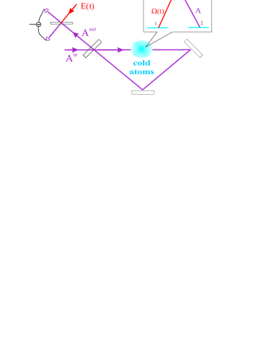
Figure 1: (Color online) Quantum memory set-up: field $A^{in}$ is sent into a cavity containing an ensemble of three-level atoms. The coupling of the intracavity field $A(t)$ with the atomic ground state variables is dynamically controlled by a pulsed coherent field $\Omega(t)$. The fluctuations of the output field $A^{out}$ are measured by homodyning with a local oscillator $E(t)$, the temporal profile of which may be adjusted so as to optimize the detection efficiency.

Our aim is to study the dynamics of light fluctuations during write and read sequences into a quantum memory. The physical system that we use as a quantum memory is the collective ground-state spin associated to two ground-state sublevels of $\Lambda$-type atoms (Fig. 1). The atoms interacts with a coherent control field on one optical transition - with Rabi frequency $\Omega(t)$, and with a field $A(t)$ possessing non-classical fluctuations on the other transition. Since we are only interested in this paper in the temporal aspects of the absorbed or emitted field modes, we neglect all spatial dependence - either longitudinal or transverse - of the fields and we assume that the atoms are enclosed in an optical cavity - with relatively low finesse.

To simplify the analysis we consider that the incoming field $A^{in}(t)$ on the cavity is a broadband squeezed vacuum and that a control field pulse with envelope $\Omega(t)$ (starting at $t=-\infty$ and assumed real) is injected into the cavity. In this case, since the vacuum field is defined with respect to the control field, its temporal mode is precisely given by the control field envelope. If we denote by $A(t)$ the annihilation operator associated to the cw multimode squeezed field, the annihilation operator associated to the incident write pulse is defined as grosshans

$$\tilde{A}^{in}\equiv\frac{\int dt\;\Omega(t)A^{in}(t)}{\sqrt{\int dt\;\Omega(t)^{2}}},$$ (1)

the normalization being such that $[\tilde{A}^{in},\;\tilde{A}^{in\dagger}]=1$.

The $N$ atoms are initially prepared in a coherent spin state: $\langle J_{z}\rangle=N/2$ and $\Delta J_{x}^{2}(-\infty)=\Delta J_{y}^{2}(-\infty)=N/4$, where $J_{z}=(\Pi_{2}-\Pi_{1})/2$ is the ground-state population difference and $J_{x}$, $J_{y}$ are the real and imaginary parts of the ground-state coherence $J=\sum_{i}|2\rangle_{i}\langle 1|_{i}$. Since the squeezed field amplitude mean value is zero this state is stationary for the mean values (assuming one neglects the ground-state spin depolarization during the write and read pulse). The ground-state spin quantum state is then given by the fluctuations of $J_{x}$ and $J_{y}$, which play a role similar to that of the field quadratures $X=A+A^{\dagger}$ and $Y=i(A^{\dagger}-A)$. The atomic fluctuations are then only coupled to the squeezed vacuum field when the control field is applied and it can be shown that the vacuum field fluctuations are decoupled from those of the control field memoire

$$\delta\dot{A} = -\kappa\delta A+\frac{ig}{\tau}\delta P+\sqrt{\frac{2\kappa}{\tau}}\delta A^{in}$$ (2)

$$\delta\dot{P} = -\gamma\delta P+i\Omega\delta J+igN\delta A+F$$ (3)

$$\delta\dot{J} = \;i\Omega\delta P$$ (4)

In order to optimize the quantum state transfer efficiency we have assumed an EIT-type interaction (one- and two-photon resonance) with a resonant cavity. $\gamma$ is the optical dipole relaxation rate, $g$ the atom-field coupling constant, $\kappa$ and $\tau$ the cavity bandwidth and the cavity round-trip time, respectively. $F$ is a Langevin atomic noise operator accounting for the spontaneous emission that degrades the squeezing transfer. The squeezing bandwidth is assumed to be broad with respect to the atomic spectral response which will be defined later on.

We now assume that the interaction parameters are chosen such that the intracavity field and the optical dipole evolve rapidly with respect to the ground-state observables. As shown in Ref. memoire , this means that the effective atomic relaxation rate satisfy at all times,

$$\tilde{\gamma}(t)=\frac{\Omega^{2}(t)}{\gamma(1+2C)},$$ (5)

should satisfy

$$\gamma_{0}\ll\tilde{\gamma}(t)\ll\gamma,\kappa$$ (6)

with $\gamma_{0}$ the ground-state decay rate. In this case, the atomic ground-state coherence fluctuations are linearly coupled to the incident field fluctuations

$$\delta\dot{J}_{x}(t) = -\tilde{\gamma}(t)\delta J_{x}(t)-\beta_{E}(t)\delta X^{in}(t)+\tilde{f}_{x}(t),$$ (7)

while the outgoing field fluctuations - $\delta A^{out}=\sqrt{\mathcal{T}}\delta A-\delta A^{in}$ - adiabatically follow the atomic fluctuations

$$\delta X^{out}(t) = \frac{1-2C}{1+2C}\delta X^{in}(t)-\frac{4\beta_{E}(t)}{N}\delta J_{x}(t)$$ (8)

$$\hskip 56.9055pt-\frac{4g}{\gamma\sqrt{\mathcal{T}}(1+2C)}F_{y}(t)$$

with

$$\beta_{E}(t)=\frac{gN\Omega(t)}{\gamma\sqrt{\mathcal{T}}(1+2C)},\hskip 14.22636pt\tilde{f}_{x}(t)=-\frac{\Omega(t)}{\gamma(1+2C)}F_{y}(t),$$

and $\mathcal{T}=2\kappa\tau$ is the intensity transmission of the coupling mirror, $C=g^{2}N/\gamma\mathcal{T}$ is the cooperativity parameter. Similar equations relate the orthogonal spin component $J_{y}$ to the incoming and outgoing field orthogonal quadrature $Y^{in}$ and $Y^{out}$ memoire .

III Writing: atomic squeezing build-up

Because of the linear coupling between the squeezed incident field quadratures and the atomic spin components, the field squeezing is transferred to the atoms during the writing phase. If we consider an incident amplitude squeezed field with a two-time correlation function of the form

$$\langle\delta X^{in}(t)\delta X^{in}(t^{\prime})\rangle=e^{-2r}\delta(t-t^{\prime}),$$ (9)

it means that the variance of the squeezed pulse is given by

$$\Delta^{2}\tilde{X}^{in}=\frac{\int dtdt^{\prime}\;\Omega(t)\Omega(t^{\prime})\langle\delta X^{in}(t)\delta X^{in}(t^{\prime})\rangle}{\int dt\;\Omega^{2}(t)}=e^{-2r},$$

consistently with our assertion that the control field envelope defines the squeezed vacuum pulse temporal profile.
Integrating (7) yields the normalized atomic variance - $\Delta\bar{J}_{x}^{2}(t)\equiv\Delta J_{x}^{2}(t)/(N/4)$ - of the $J_{x}$ component at time $t$

$$\Delta\bar{J}_{x}^{2}(t)=e^{-2a(t)}+[1-e^{-2a(t)}]\left(\eta e^{-2r}+1-\eta\right)$$ (10)

with

$$a(t)=\int_{-\infty}^{t}dt^{\prime}\tilde{\gamma}(t^{\prime})=\tilde{\gamma}_{0}\int_{-\infty}^{t}dt^{\prime}\xi(t^{\prime})$$ (11)

where $\tilde{\gamma}_{0}=\Omega(0)^{2}/\gamma(1+2C)$ is the static effective relaxation rate of Ref. memoire , $\xi(t)$ is the normalized envelope of the intensity of the pulse and $\eta=2C/(1+2C)$ is the static quantum state transfer efficiency of memoire . To evaluate the dynamical build-up of the atomic squeezing, one should compare the normalized atomic noise reduction $1-\Delta\bar{J}_{x}^{2}$ to the incident field squeezing $1-e^{-2r}$. Taking for the control pulse a centered Gaussian profile $\xi(t)=e^{-t^{2}/T^{2}}/\sqrt{\pi}$ of duration $T$, the quantum state transfer efficiency at time $t$ is given by

$$\eta_{w}(t)\equiv\frac{1-\Delta\bar{J}_{x}^{2}(t)}{1-e^{-2r}}=\eta[1-e^{-2a(t)}]$$ (12)

The atomic squeezing increases exponentially with the integrated intensity of the pulse $a(t)$. In steady state ($t\gg T$), the writing quantum efficiency is simply

$$\eta_{w}=\eta(1-e^{-2a(\infty)})=\eta(1-e^{-2\tilde{\gamma}_{0}T})$$ (13)

The efficiency $\eta_{w}$ approaches the cw efficiency $\eta$ when the total pulse “area” $a(\infty)$ is large with respect to 1 (Fig. 4). One recovers the results of Ref. memoire - $\eta_{w}\sim\eta$ - when the pulse duration is long with respect to the effective atomic response time $1/\tilde{\gamma}_{0}$, which justifies our previous assertion that $\eta$ is the cw transfer efficiency. Physically, the squeezing transfer does not depend on the profile of the write pulse and is high when the cooperativity is large ($\eta\sim 1$), the pulse “area” is large enough and the incident squeezing bandwidth is large with respect to $\tilde{\gamma}_{0}$.

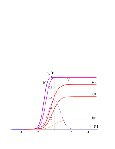
Figure 2: (Color online) “Write” efficiency $\eta_{w}(t)$ (normalized to $\eta$) versus time $t/T$, when the write pulse “area” increases [Gaussian envelopes with (a) $a(\infty)=0.1$ (b) 0.5 (c) 1 (d) 5 (e) 10]. The dashed curve represents the write pulse envelope $\xi(t)$.

IV Readout

IV.1 Outgoing field fluctuations

In order to readout the atomic state after the squeezing has been stored, one can reapply - after a variable storage time - the coherent control field, the incident squeezed field being now turned off. The reverse process takes place and the atoms, initially squeezed, now transfer their squeezing to the intracavity field. This squeezing in turn reflects in the field exiting the cavity. The evolution is still given by (7-8), but with the initial conditions

$$\langle\delta X^{in}(t)\delta X^{in}(t^{\prime})\rangle=\delta(t-t^{\prime}),\hskip 11.38092pt\Delta\bar{J}_{x}^{2}(-\infty)=e^{-2r}$$

The outgoing field two-time correlation function can be shown to be

$$\mathcal{C}(t,t^{\prime}) \equiv \langle\delta X^{out}(t)\delta X^{out}(t^{\prime})\rangle$$ (14)

$$= \delta(t-t^{\prime})+\eta f(t)f(t^{\prime})(e^{-2r}-1)$$ (15)

with

$$f(t)=\sqrt{2\tilde{\gamma}(t)}e^{-a(t)}$$ (16)

The $\delta$-correlated term corresponds to the vacuum field contribution that one would have without atoms or control field. The second term carries the stored atomic squeezing with a certain temporal profile and shows that the outgoing field will be transitorily squeezed. The essential result is that this temporal profile always differs from that of the readout pulse, which means that the squeezing (and, by extension, the non-classical fluctuations) is emitted in a different temporal mode. As can be seen from Fig. 3, the field radiated by the collective atomic dipole results in an outgoing field envelope with a different shape than the read pulse. The maximum of emission occurs at a time $-t_{0}$ different than the read pulse maximum. For a Gaussian read pulse envelope, $f(t)\propto e^{-[t^{2}/T^{2}+\tilde{\gamma}_{0}T(1+\small{\textrm{erf}}[t/T])]/2}$ and $t_{0}/T=\sqrt{PL(2\tilde{\gamma}_{0}^{2}T^{2}/\pi)/2}$ where $PL$ denotes the product-log function. The delay between the emitted field and the read pulse increases with the pulse area and may be understood with the help of the toy model of Sec. VI.

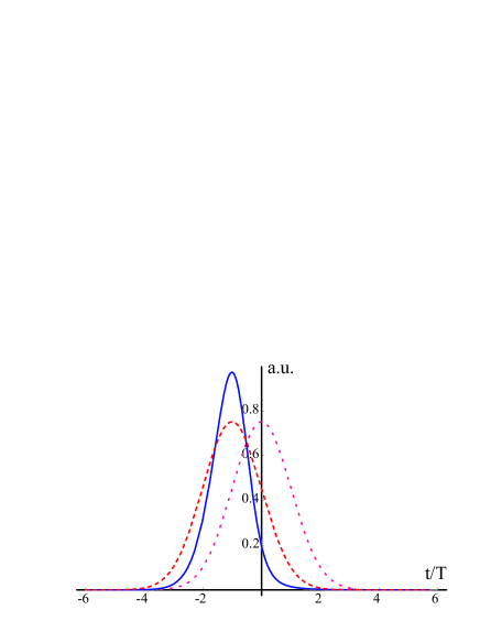
Figure 3: (Color online) Radiated pulse (plain), read pulse (dotted) and delayed read pulse (dashed) envelopes vs time $t/T$, for $\tilde{\gamma}_{0}T=5$.

IV.2 Homodyning with the read pulse

We now give an operational definition of the outgoing field pulse noise measurement. We assume that its fluctuations are measured by homodyning with a local oscillator with a temporal profile $\mathcal{E}(t)$. The measurement operator is then defined as

$$\tilde{X}^{out}\equiv\frac{\int dt\;\mathcal{E}(t)X^{out}(t)}{\sqrt{\int dt\;\mathcal{E}(t)^{2}}},$$ (17)

and its noise properties are calculated using the correlation function (14)

$$\Delta^{2}\tilde{X}^{out} = \frac{\int dtdt^{\prime}\;\mathcal{E}(t)\mathcal{E}(t^{\prime})\mathcal{C}(t,t^{\prime})}{\int dt\;\mathcal{E}(t)^{2}}$$

$$= 1+\eta(e^{-2r}-1)\frac{\left[\int dt\;\mathcal{E}(t)f(t)\right]^{2}}{\int dt\;\mathcal{E}(t)^{2}}.$$

and the readout efficiency is defined in a similar fashion as the write efficiency by

$$\eta_{r}\equiv\frac{1-\Delta^{2}\tilde{X}^{out}}{1-e^{-2r}}.$$ (18)

An experimentally simple and natural way to measure the field squeezing would be to use a local oscillator (LO) that would be (matched with) the control field read pulse and suitably delayed: $\mathcal{E}(t)\propto\Omega(t+t_{0})$. Choosing $t_{0}$ such that the overlap is maximum between both pulses, the readout efficiency is optimal - $\eta_{r}^{*}\simeq 0.96$ - when the pulse duration is such that $\tilde{\gamma}_{0}T^{*}\simeq 2.5$ (Fig. 4). However, when the pulse duration is increased, the readout pulse squeezing decreases. This imperfect efficiency can be explained by the fact that the local oscillator in $\Omega(t+t_{0})$ does not perfectly matches the atomic emission in $f(t)$ (Fig. 3). This result implies that for a practical implementation with fixed pulse duration, the read pulse “area” $a(\infty)$ should not be too large in order to optimize the readout. This is in contrast with the write sequence, for which a large “area” pulse is preferable.

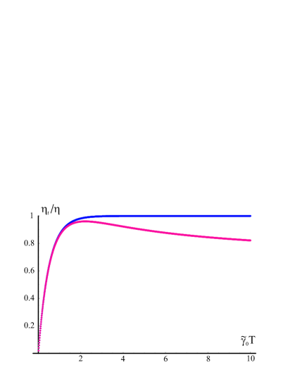
Figure 4: (Color online) Readout efficiency $\eta_{r}$ (normalized by the cw efficiency $\eta$) versus pulse “area” $a(\infty)=\tilde{\gamma}_{0}T$ when the LO is either the retarded readout pulse (lower curve) or a pulse temporally matched with the atomic emission (upper curve).

IV.3 Temporal matching

It is possible however to measure the totality of the initial atomic squeezing if one matches the LO temporal profile with that of the field radiated by the atoms memoire ; molmer : $\mathcal{E}(t)=\sqrt{2\tilde{\gamma}(t)}e^{-a(t)}$. In this case, the measured field variance is then

$$\Delta^{2}\tilde{X}^{out}=1+\eta[1-e^{-2a(\infty)}](e^{-2r}-1)$$ (19)

The shot-noise is given by $\mathcal{N}=[1-e^{-2a(\infty)}]$ and, if one uses the same pulse to write and read, the readout efficiency is equal to the writing efficiency

$$\eta_{r}=\eta[1-e^{-2a(\infty)}].$$ (20)

In contrast with the previous readout method using the read pulse as a local oscillator, the readout efficiency increases when the pulse area is increased.

Note also that when $T$ is large with respect to the atomic response time $\tilde{\gamma}_{0}^{-1}$, one recovers the cw case of Ref. memoire , in which the constant readout field is abruptly applied at $t=0$ - the readout pulse envelope is a step function $\Omega(t)=\Theta(t)\Omega$ - which yields a correlation function of the form

$$\mathcal{C}(t,t^{\prime})=\delta(t-t^{\prime})+2\eta\tilde{\gamma}_{0}e^{-\tilde{\gamma}(t+t^{\prime})}(e^{-2r}-1)$$ (21)

The use of a local oscillator with a profile $\mathcal{E}(t)=\Theta(t)\sqrt{2\tilde{\gamma}_{0}}e^{-\tilde{\gamma}_{0}t}$ was shown to optimize the spectrum analyzer measurement, the noise power integrated over a time long with respect to $\tilde{\gamma}_{0}^{-1}$ being the sum of a shot-noise term $\mathcal{N}$ and a signal term $\mathcal{S}$ proportional to the initial atomic squeezing:

$$P=\mathcal{N}+\mathcal{S}(e^{-2r}-1)$$ (22)

When the integrating time is large with respect to $\tilde{\gamma}_{0}^{-1}$, one has $\mathcal{S}\sim\eta\mathcal{N}$, and thus a readout efficiency equal to $\eta$. In agreement with this result, we can compute the outgoing pulse variance measured with the same temporally matched LO and retrieve the same result

$$\Delta^{2}\tilde{X}^{out}=1+\eta(e^{-2r}-1)\simeq e^{-2r}\hskip 11.38092pt(\eta\sim 1)$$

IV.4 Optimal readout

One can easily show that matching the temporal modes of the local oscillator and the field radiated by the atoms provides the best readout method. Indeed, for a correlation function of the form (15), the readout efficiency can be expressed as

$$\eta_{r}=\eta\frac{\left[\int dt\;\mathcal{E}(t)f(t)\right]^{2}}{\int dt\;\mathcal{E}(t)^{2}}=\eta\frac{\langle\mathcal{E}|f\rangle^{2}}{\langle\mathcal{E}|\mathcal{E}\rangle}$$ (23)

where $\langle.|.\rangle$ denotes the hermitian scalar product

$$\langle f|g\rangle=\int dtf(t)^{*}g(t)=\int\frac{d\omega}{2\pi}f(\omega)^{*}g(\omega)$$ (24)

In this picture, an imperfect matching between the field to be measured and the local oscillator translates into an effective efficiency for the homodyne detector grosshans . Optimizing the efficiency is clearly equivalent to maximize the overlap between the local oscillator and the atomic emission, which yields at best

$$\eta_{r}^{*}=\eta\langle f|f\rangle$$ (25)

when $|\mathcal{E}\rangle=|f\rangle$. The best efficiency is thus obtained when $\langle f|f\rangle=1$. With $f$ of the form (16), this corresponds to a constant intensity profile for the readout pulse, such as the one of Ref. memoire , or pulses of duration $T$ such that $a(\infty)\gg 1$. Let us insist on the fact that, if it is possible to retrieve the totality of the information on the atomic state, the fluctuations of the field radiated during the readout sequence always have a different temporal profile than the write pulse.

We would like to point out that this approach - which yields convenient mathematical quantities also gives the truly physically interesting observables for quantum information processing, as for instance in a quantum teleportation protocol. Using the atomic teleportation protocol of Ref. telep it follows from the previous results that the optimal gain to teleport non-classical atomic fluctuations should have a temporal profile matching the atomic emission $f(t)$. The retrieved temporal modes takes on in this case a clear operational definition in terms of optimizing the teleported fluctuations.

V Writing and no-cloning theorem

It is also interesting to look at what happens to the outgoing field during the writing phase. The two-time correlation function reads

$$\mathcal{C}(t,t^{\prime}) = \delta(t-t^{\prime})+(e^{-2r}-1)[(2\eta-1)^{2}\delta(t-t^{\prime})$$

$$+2\eta(1-\eta)\sqrt{\tilde{\gamma}(t)\tilde{\gamma}(t^{\prime})}e^{-|a(t)-a(t^{\prime})|}-\eta^{2}f(t)f(t^{\prime})]$$

When $\eta\sim 1$, the variance measured with the matched local oscillator $\mathcal{E}(t)=f(t)$ is simply given by

$$\Delta^{2}\tilde{X}^{out}(t)=e^{-2r}+(1-e^{-2r})\mathcal{N}(t),$$

with $\mathcal{N}(t)=1-e^{-2a(t)}$, so that, at all times, one has note

$$\Delta\bar{J}^{2}_{x}(t)+\Delta^{2}\tilde{X}^{out}(t)=1+e^{-2r}.$$

In this picture, this process clearly appears as the quantum state transfer from one mode to another

$$\Delta\bar{J}_{x}^{2}(-\infty) = 1,\hskip 19.91684pt\Delta^{2}\tilde{X}^{out}(-\infty)=e^{-2r}$$

$$\Delta\bar{J}_{x}^{2}(+\infty) = e^{-2r},\hskip 5.69046pt\Delta^{2}\tilde{X}^{out}(+\infty)=1.$$

In agreement with the no-cloning theorem wootters , the field squeezing disappears while the atoms become squeezed, meaning that the initial copy is indeed destroyed during the write sequence.

VI Analogy with a cavity with variable transmission

The atomic memory behavior can actually be modeled in a very simple fashion by considering an empty cavity, the transmission of which is controllable: $\mathcal{T}(t)=2\kappa(t)\tau$ transmission . With the same convention as previously, the input-output relations for the field read

$$\tau\delta\dot{A}(t) = -\frac{\mathcal{T}(t)}{2}\delta A(t)+\sqrt{\mathcal{T}(t)}\delta A^{in}(t)$$ (26)

$$\delta A^{out}(t) = \sqrt{\mathcal{T}(t)}\delta A(t)-\delta A^{in}(t)$$ (27)

During the write sequence the incident field is squeezed, while the intracavity field is in a vacuum state:

$$\langle\delta X^{2}(-\infty)\rangle=\frac{1}{\tau},\hskip 11.38092pt\langle\delta X^{in}(t)\delta X^{in}(t^{\prime})\rangle=\delta(t-t^{\prime})e^{-2r}$$

Integrating Eq. (26), one gets the intracavity field variance at time $t$

$$\langle\delta X^{2}(t)\rangle=\frac{1}{\tau}\left[e^{-2r}+(1-e^{-2r})e^{-2a(t)}\right]$$ (28)

with $a(t)=\int_{-\infty}^{t}ds\;\kappa(s)$, which has exactly the same form as the atomic variance in Eq. (10) when $\eta=1$ and $\tilde{\gamma}(t)$ is replaced by $\kappa(t)$. When the incident pulse area is large - $a(\infty)\gg 1$ - the intracavity field is perfectly squeezed when the transmission vanishes. The squeezing is then stored into a closed cavity with infinite lifetime lifetime .

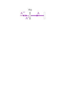
Figure 5: Cavity with variable transmission.

During the readout phase, one reopens the cavity by varying again $\mathcal{T}(t)$. After integration with the initial conditions

$$\langle\delta X^{2}(-\infty)\rangle=\frac{e^{-2r}}{\tau},\hskip 11.38092pt\langle\delta X^{in}(t)\delta X^{in}(t^{\prime})\rangle=\delta(t-t^{\prime})$$

the two-time correlation function of the outgoing field takes on the same form as in Eq. (15), with, again, $\eta=1$ and $\tilde{\gamma}(t)$ replaced by $\kappa(t)$:

$$\mathcal{C}(t,t^{\prime})=\delta(t-t^{\prime})+f(t)f(t^{\prime})(e^{-2r}-1)$$ (29)

with $f(t)=\sqrt{2\kappa(t)}e^{-\int_{-\infty}^{t}ds\;\kappa(s)}$. Within this formalism, the atomic memory considered here is clearly equivalent to an infinite lifetime storage cavity. The characteristics of the field emitted during readout, the transfer efficiencies, the detection strategies are the same as for the atomic memory case. The CV quantum memory can then be characterized using the general methods developed previously. For instance, the squeezing leaks out of the cavity as soon as the transmission becomes non-zero, so that its envelope $f(t)$ is different of the transmission profile $\mathcal{T}(t)$. The maximum of emission $t_{0}$ indeed depends on the transmission of the cavity at time $t_{0}$ as well as the amount of squeezing that has already left the cavity. This toy model also gives a simple interpretation for the control field in the atomic memory scheme, which plays the same role as a “tap” which couples or decouples the stored squeezing to the outside.

VII Conclusion

We have studied the temporal mode-matching conditions for an optimal transfer of quantum fluctuations between optical fields and an atomic ensemble collective spin. These conditions stress the relevant physical quantities involved in the quantum state transfer process in cw or in pulsed schemes. Not only do they provide an operational meaning of the quantum states exchanged between the fields and the atoms, but, owing to the different temporal modes involved in the write and read sequences, they also show how the non classical states generated in the pulsed regime wenger can be to measured and utilized experimentally in continuous variable protocols such as teleportation for instance telep .

We would like to point out that these results - in particular, the simple toy model of Sec. VI - can easily be extended to other storage media which can be used as continuous variable quantum memories, such as movable mirrors or nuclear spins pinard ; helium . In particular, a consequence for practical implementations of continuous variable memories is that, regardless of the storage medium, different strategies regarding the characteristics of the read pulse can be adopted to readout the memory.

Note also that the results derived here for squeezing are actually valid for EPR-type entanglement or any Gaussian non-classical fluctuations. Let us remark that the analysis developed in this paper, in particular, he fact that quantum fluctuations are preserved, is the analogous for the CV regime of the conservation of the quantum character of the field in the single photon experiments singlephoton .

Last, in the case of an atomic memory, it would also be interesting to look at how propagation effects will affect these results in a scheme without cavity singlephoton ; simplepassage ; akamatsu .

- (1) M.D. Lukin, Rev. Mod. Phys. 75, 457 (2003).
- (2) L.M. Duan, M.D. Lukin, J.I. Cirac, P. Zoller, Nature (London) 414, 413 (2001).
- (3) B. Julsgaard et al., Nature (London) 413, 400 (2001).
- (4) C.H. van der Wal et al., Science 301, 196 (2003).
- (5) D.N. Matsukevitch and A. Kuzmich, Science 306, 663 (2004).
- (6) C.W. Chou et al., Phys. Rev. Lett. 92, 213601 (2004).
- (7) M.D. Eisaman et al., Phys. Rev. Lett. 93, 233602 (2004); S.V. Polyakov et al., Phys. Rev. Lett. 93, 263601 (2004).
- (8) C. Liu et al., Nature (London) 409, 490 (2001); D.F. Phillips et al., Phys. Rev. Lett. 86, 783 (2001); M. Bajcsy et al., Nature (London) 426, 633 (2004).
- (9) L.M. Duan, J.I. Cirac, P. Zoller, E.S. Polzik, Phys. Rev. Lett. 85, 5643 (2000).
- (10) T. Chaneliere et al., Nature (London) 438, 833 (2005); M.D. Eisaman et al., Nature (London) 438, 837 (2005).
- (11) B. Julsgaard et al., Nature (London) 432, 482 (2004).
- (12) M.D. Lukin and M. Fleischhauer, Phys. Rev. Lett. 84, 5094 (2000).
- (13) A. Kozhekin, K. Mølmer, E.S. Polzik, Phys. Rev. A 62, 33809 (2001).
- (14) A. Dantan and M. Pinard, Phys. Rev. A 69, 43810 (2004); A. Dantan, A. Bramati, M. Pinard, Europhys. Lett. 67, 881 (2004).
- (15) A.S. Parkins and H.J. Kimble, J. Opt. B: Quantum and Semiclass. Opt. 1, 496 (1999).
- (16) J. Zhang, K.C. Peng, S.L. Braunstein, Phys. Rev. A 68, 13808 (2003).
- (17) M. Pinard et al., Europhys. Lett. 72, (2005).
- (18) A. Dantan et al., Phys. Rev. Lett. 95, 123002 (2005).
- (19) J. Wenger, R. Tualle-Brouri, P. Grangier, Opt. Lett. 29, 1267 (2004); J. Wenger, A. Ourjoumtsev, R. Tualle-Brouri, P. Grangier, Eur. Phys. J. D 32, 391 (2005).
- (20) F. Grosshans and P. Grangier, Eur. Phys. J. D 14, 119 (2001).
- (21) U.V. Poulsen and K. Mølmer, Phys. Rev. Lett. 87, 123601 (2001).
- (22) A. Dantan, N. Treps, A. Bramati, M. Pinard, Phys. Rev. Lett. 94, 050502 (2005).
- (23) This may also correspond to a variation of the cavity length, if one inserts a Pockels cell and a birefringent element inside the cavity for instance.
- (24) with .
- (25) W.K. Wootters and W.H. Zurek, Nature (London) 299, 802 (1982).
- (26) A finite lifetime could easily be included by adding a small transmission to the second mirror for instance.
- (27) A. Dantan, A. Bramati, M. Pinard, Phys. Rev. A 71, 43801 (2005).
- (28) D. Akamatsu, K. Akiba, M. Kozuma, Phys. Rev. Lett. 92, 203602 (2004).