Implementation of quantum logic operations
and creation of entanglement
in a silicon-based quantum computer with constant interaction

Abstract

We describe how to implement quantum logic operations in a silicon-based quantum computer with phosphorus atoms serving as qubits. The information is stored in the states of nuclear spins and the conditional logic operations are implemented through the electron spins using nuclear-electron hyperfine and electron-electron exchange interactions. The electrons in our computer should stay coherent only during implementation of one Control-Not gate. The exchange interaction is constant and selective excitations are provided by a magnetic field gradient. The quantum logic operations are implemented by rectangular radio-frequency pulses. This architecture is scalable and does not require manufacturing nanoscale electronic gates. As shown in this paper parameters of a quantum protocol can be derived analytically even for a computer with a large number of qubits using our perturbation approach. We present the protocol for initialization of the nuclear spins and the protocol for creation of entanglement. All analytical results are tested numerically using a two-qubit system.

I Introduction

The long decoherence time of nuclear spins of phosphorus donors in silicon makes quantum computers based on these spins attractive for quantum information processing. A scanning tunneling microscopy technique 1994 ; 1996 ; surfSci ; electronics ; clark can be used for creation of many identical arrays of phosphorus atoms on the (100) surface of silicon. The phosphorus qubits can be encapsulated by overgrowing additional silicon layers clark to increase the electron relaxation time. Kane kane proposed to use nanoscale electronic gates to control the qubits. This technique has not yet been realized, due to fabrication issues, and so in this paper we consider a different architecture. In our approach, the exchange interaction between qubits is constant and selective interactions are realized through the use of a magnetic field gradient and both microwave and radio frequency pulses. Measurement can be implemented using optical techniques optical1 ; optical2 ; optical3 . The measurement can be facilitated by creation of many identical, noninteracting spin chains to amplify the signal.

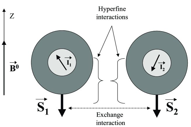
Figure 1: A schematic illustration of two phoshorus atoms placed in a permanent magnetic field $\vec{B}^{0}$. The electron spins $\vec{S}_{1}$ and $\vec{S}_{2}$ (large arrows) of the neigboring atoms interact with each other via the exchange interaction and the nuclear spins $\vec{I}_{1}$ and $\vec{I}_{2}$ (small arrows) interact with the electron spins through the hyperfine interactions.

The ³¹P atom has electron spin 1/2 and nuclear spin 1/2. If the qubits in each chain are placed at a separation of $\sim$ 10 nm from each other, the nuclear-nuclear, nuclear-electron, and electron-electron dipole-dipole interactions are small compared to the electron-electron exchange interaction so that one can neglect the dipole-dipole interactions (see Fig. 1). There is also a relatively strong hyperfine interaction between the electron and nuclear spins of a ³¹P atom. Since the relaxation time for the electron spins at temperatures of 1-7 K is relatively small (0.6-60 ms at 7 K T_c ), the quantum information must be stored in the states of the nuclear spins. Because the nuclear spins do not interact, electron spins can be used to mediate the nuclear-nuclear interactions. In this setup, the electron spins must be coherent only during the relatively short time of implementation of a quantum logic gate, such as a Control-Not gate, on a particular pair of qubits.

We consider in this paper a procedure for implementation of entanglement between the nuclear spins in a two-qubit quantum computer using rectangular radio-frequency pulses. Entanglement is the simplest quantum logic operation needed for implementation of more complex quantum logic gates and is useful for demonstration of quantum computation in a potentially scalable solid-state system. The paper is organized as follows. The eigenstates of the system are calculated analytically in Section II. A brief description of the protocol for creation of entanglement is given in Section III. The quantum dynamics of the system is described in Section IV. The eigenstates from Section II are used for calculation of pulse parameters in Section V. Initialization and entanglement with two qubits are simulated numerically in Section VI. In Section VII we review the working conditions and the parameter range for our computer.

II Eigenstates

The unperturbed Hamiltonian of the system reads

$$\hat{H}^{0}=\gamma_{e}B_{1}^{z}\hat{S}_{1}^{z}+\gamma_{e}B_{2}^{z}\hat{S}_{2}^{z}-\gamma_{n}B_{1}^{z}\hat{I}_{1}^{z}-\gamma_{n}B_{2}^{z}\hat{I}_{2}^{z}+$$

$$A\left[\hat{S}_{1}^{z}\hat{I}_{1}^{z}+\hat{S}_{2}^{z}\hat{I}_{2}^{z}+{1\over 2}\left(\hat{S}_{1}^{+}\hat{I}_{1}^{-}+\hat{S}_{1}^{-}\hat{I}_{1}^{+}+\hat{S}_{2}^{+}\hat{I}_{2}^{-}+\hat{S}_{2}^{-}\hat{I}_{2}^{+}\right)\right]+J\left[\hat{S}_{1}^{z}\hat{S}_{2}^{z}+{1\over 2}\left(\hat{S}_{1}^{+}\hat{S}_{2}^{-}+\hat{S}_{1}^{-}\hat{S}_{2}^{+}\right)\right],$$

where $\hat{S}_{k}^{\alpha}$ ($\hat{I}_{k}^{\alpha}$) is the projection of the $k$th electron (nuclear) spin on the $\alpha$th axis, $k=1,2$, $\alpha=x,y,z$; $\hat{S}^{\pm}_{k}=\hat{S}^{x}_{k}\pm i\hat{S}^{y}_{k}$, $\hat{I}^{\pm}_{i}=\hat{I}^{x}_{k}\pm i\hat{I}^{y}_{k}$; $\gamma_{e}$ and $\gamma_{n}$ are, respectively, the electron and nuclear gyromagnetic ratios; $B_{k}^{z}$ is the permanent magnetic field in the location of the $k$th spin; $A$ and $J$ are, respectively, the hyperfine and exchange interaction constants.

Let us define

$$\hat{\Sigma}=\hat{S}_{1}^{z}+\hat{S}_{2}^{z}+\hat{I}_{1}^{z}+\hat{I}_{2}^{z}.$$

The quantum states form 5 independent subspaces characterized by the value of

$$\Sigma_{n}=\langle\psi_{n}|\hat{\Sigma}|\psi_{n}\rangle.$$

Two one-dimensional subspaces with $\Sigma_{n}=\pm 2$ are formed by the eigenstates with the following eigenvalues $E_{n}$ and eigenvectors $|\psi_{n}\rangle$:

$$E_{15}={1\over 2}\left(-\gamma_{e}B_{1}^{z}-\gamma_{e}B_{2}^{z}+\gamma_{n}B_{1}^{z}+\gamma_{n}B_{2}^{z}\right)+{A\over 2}+{J\over 4}=\left(-\gamma_{e}+\gamma_{n}\right)b+{A\over 2}+{J\over 4},$$ (1)

$$|\psi_{15}\rangle=|\downarrow_{2}\,\Downarrow_{2}\,\Downarrow_{1}\,\downarrow_{1}\,\rangle,$$ (2)

$$E_{0}=\left(\gamma_{e}-\gamma_{n}\right)b+{A\over 2}+{J\over 4},~{}~{}~{}|\psi_{0}\rangle=|\uparrow_{2}\,\Uparrow_{2}\,\Uparrow_{1}\,\uparrow_{1}\,\rangle,$$ (3)

where $b=(B_{2}^{z}+B_{1}^{z})/2$ and we use the notation $|\Uparrow_{k}\rangle$ and $|\Downarrow_{k}\rangle$ for the states of the electron spins and $|\uparrow\rangle_{k}$ and $|\downarrow\rangle_{k}$ for the states of the nuclear spins, $k=1,2$.

The basis vectors for the subspace with $\Sigma_{n}=-1$ are

$$\left(\begin{array}[]{c}|\downarrow_{2}\,\Downarrow_{2}\,\Uparrow_{1}\,\downarrow_{1}\,\rangle\\ |\downarrow_{2}\,\Uparrow_{2}\,\Downarrow_{1}\,\downarrow_{1}\,\rangle\\ |\downarrow_{2}\,\Downarrow_{2}\,\Downarrow_{1}\,\uparrow_{1}\,\rangle\\ |\uparrow_{2}\,\Downarrow_{2}\,\Downarrow_{1}\,\downarrow_{1}\,\rangle\\ \end{array}\right)=\left(\begin{array}[]{c}|13\rangle\\ |11\rangle\\ |14\rangle\\ |7\rangle\\ \end{array}\right).$$ (4)

Introducing the notation $\delta B=(B_{2}^{z}-B_{1}^{z})/2$ the Hamiltonian matrix for $\Sigma_{n}=-1$ becomes

$$\left(\begin{array}[]{cccc}-\gamma_{e}\delta B+\gamma_{n}b-{J\over 4}&{J\over 2}&{A\over 2}&0\\ {J\over 2}&\gamma_{e}\delta B+\gamma_{n}b-{J\over 4}&0&{A\over 2}\\ {A\over 2}&0&-\gamma_{e}b+\gamma_{n}\delta B+{J\over 4}&0\\ 0&{A\over 2}&0&-\gamma_{e}b-\gamma_{n}\delta B+{J\over 4}\end{array}\right).$$ (5)

This matrix can be diagonalized analytically. For $\delta B=0$ the eigenvalues and eigenfunctions were found in Ref. 2000 . Instead of the exact analytical solution we apply here a perturbative approach. Our perturbative approach has an advantage over the exact analytical solution because it can be used to find the eigenstates for the quantum computer with more than two qubits when no exact analytical solution is available. The perturbation theory is based on the fact that $\gamma_{e}b$ is at least three orders of magnitude larger than $J/4$, $A/2$, $\gamma_{e}\delta B$, $\gamma_{n}b$, and $\gamma_{n}\delta B$. (We take $b\approx 3.3$ T so that $\gamma_{e}b/(2\pi)\approx 93$ GHz, $J/(2\pi)\approx 1-10$ MHz or less, $A/(2\pi)=116$ MHz.) For our range of parameters the matrix (5) splits into two relatively independent $2\times 2$ blocks PRA01 ; JAM . The first block is formed by the matrix elements in the upper left corner and the second block is formed in the lower right corner. The relative independence of the two different blocks follows from the facts that (a) the moduli of the differences between the eigenvalues of each block are much smaller than the moduli of the differences ($\sim\gamma_{e}b$) between the eigenvalues of the different blocks; and (b) the matrix elements $A/2$ relating the different blocks are much smaller than $\gamma_{e}b$. The corrections to the wave function due to the neglected terms are of the order of

$$\epsilon={(A/2)\over\gamma_{e}b}\approx 6\times 10^{-4}$$ (6)

and corrections $E^{(2)}_{i}$ to the energy levels $E^{(0)}_{i}$, $i=1,\dots,14$, are of the order of tens of kilohertz. These corrections are important in order to flip the nuclear spins because the Rabi frequencies of the nuclear spins are of the same magnitude.

The eigenvalues and the eigenfunctions are

$$E_{7}^{(0)}=-\gamma_{e}b-\gamma_{n}\delta B+{J\over 4},~{}~{}~{}|\psi_{7}^{(0)}\rangle=|\uparrow_{2}\,\Downarrow_{2}\,\Downarrow_{1}\,\downarrow_{1}\,\rangle,$$ (7)

$$E_{14}^{(0)}=-\gamma_{e}b+\gamma_{n}\delta B+{J\over 4},~{}~{}~{}|\psi_{14}^{(0)}\rangle=|\downarrow_{2}\,\Downarrow_{2}\,\Downarrow_{1}\,\uparrow_{1}\,\rangle,$$ (8)

$$E_{13}^{(0)}=\gamma_{n}b-{J\over 4}-\sqrt{(\gamma_{e}\delta B)^{2}+{J^{2}\over 4}},$$ (9)

$$E_{11}^{(0)}=\gamma_{n}b-{J\over 4}+\sqrt{(\gamma_{e}\delta B)^{2}+{J^{2}\over 4}}.$$ (10)

The eigenfunctions corresponding to $E_{13}^{(0)}$ and $E_{14}^{(0)}$ are

$$|\psi_{13}^{(0)}\rangle=D_{13}|\downarrow_{2}\,\rangle\otimes\left\{\left[\gamma_{e}\delta B+\sqrt{(\gamma_{e}\delta B)^{2}+{J^{2}\over 4}}\right]|\Downarrow_{2}\,\Uparrow_{1}\,\rangle-{J\over 2}|\Uparrow_{2}\,\Downarrow_{1}\,\rangle\right\}\otimes|\downarrow_{1}\,\rangle,$$ (11)

$$|\psi_{11}^{(0)}\rangle=D_{11}|\downarrow_{2}\,\rangle\otimes\left\{{J\over 2}|\Downarrow_{2}\,\Uparrow_{1}\,\rangle+\left[\gamma_{e}\delta B+\sqrt{(\gamma_{e}\delta B)^{2}+{J^{2}\over 4}}\right]|\Uparrow_{2}\,\Downarrow_{1}\,\rangle\right\}\otimes|\downarrow_{1}\,\rangle,$$ (12)

where $D_{i}$, $i=1,\dots,14$, are the normalization constants. The correction $E^{(2)}_{7}$ is calculated in Appendix A and all corrections $E^{(2)}_{i}$, $i=1,14$, are listed in Appendix B.

The basis vectors for the subspace with $\Sigma_{n}=1$ are

$$\left(\begin{array}[]{c}|\uparrow_{2}\,\Uparrow_{2}\,\Downarrow_{1}\,\uparrow_{1}\,\rangle\\ |\uparrow_{2}\,\Downarrow_{2}\,\Uparrow_{1}\,\uparrow_{1}\,\rangle\\ |\uparrow_{2}\,\Uparrow_{2}\,\Uparrow_{1}\,\downarrow_{1}\,\rangle\\ |\downarrow_{2}\,\Uparrow_{2}\,\Uparrow_{1}\,\uparrow_{1}\,\rangle\\ \end{array}\right)=\left(\begin{array}[]{c}|2\rangle\\ |4\rangle\\ |1\rangle\\ |8\rangle\\ \end{array}\right).$$

The Hamiltonian matrix for $\Sigma_{n}=1$ has the following form:

$$\left(\begin{array}[]{cccc}\gamma_{e}\delta B-\gamma_{n}b-{J\over 4}&{J\over 2}&{A\over 2}&0\\ {J\over 2}&-\gamma_{e}\delta B-\gamma_{n}b-{J\over 4}&0&{A\over 2}\\ {A\over 2}&0&\gamma_{e}b-\gamma_{n}\delta B+{J\over 4}&0\\ 0&{A\over 2}&0&\gamma_{e}b+\gamma_{n}\delta B+{J\over 4}\end{array}\right).$$ (13)

The eigenvalues and the eigenfunctions are

$$E_{1}^{(0)}=\gamma_{e}b-\gamma_{n}\delta B+{J\over 4},~{}~{}~{}|\psi_{1}^{(0)}\rangle=|\uparrow_{2}\,\Uparrow_{2}\,\Uparrow_{1}\,\downarrow_{1}\,\rangle,$$ (14)

$$E_{8}^{(0)}=\gamma_{e}b+\gamma_{n}\delta B+{J\over 4},~{}~{}~{}|\psi_{8}^{(0)}\rangle=|\downarrow_{2}\,\Uparrow_{2}\,\Uparrow_{1}\,\uparrow_{1}\,\rangle,$$ (15)

$$E_{2}^{(0)}=-\gamma_{n}b-{J\over 4}+\sqrt{(\gamma_{e}\delta B)^{2}+{J^{2}\over 4}},$$ (16)

$$E_{4}^{(0)}=-\gamma_{n}b-{J\over 4}-\sqrt{(\gamma_{e}\delta B)^{2}+{J^{2}\over 4}},$$ (17)

$$|\psi_{2}^{(0)}\rangle=D_{2}|\uparrow_{2}\,\rangle\otimes\left\{\left[\gamma_{e}\delta B+\sqrt{(\gamma_{e}\delta B)^{2}+{J^{2}\over 4}}\right]|\Uparrow_{2}\,\Downarrow_{1}\,\rangle+{J\over 2}|\Downarrow_{2}\,\Uparrow_{1}\,\rangle\right\}\otimes|\uparrow_{1}\,\rangle,$$ (18)

$$|\psi_{4}^{(0)}\rangle=D_{4}|\uparrow_{2}\,\rangle\otimes\left\{-{J\over 2}|\Uparrow_{2}\,\Downarrow_{1}\,\rangle+\left[\gamma_{e}\delta B+\sqrt{(\gamma_{e}\delta B)^{2}+{J^{2}\over 4}}\right]|\Downarrow_{2}\,\Uparrow_{1}\,\rangle\right\}\otimes|\uparrow_{1}\,\rangle.$$ (19)

The six-dimensional multiplet with $\Sigma_{n}=0$ splits into three relatively independent subspaces. The first two eigenvalues and eigenfunctions are

$$E_{6}^{(0)}=-\gamma_{e}b-\gamma_{n}b-{A\over 2}+{J\over 4},~{}~{}~{}|\psi_{6}^{(0)}\rangle=|\uparrow_{2}\,\Downarrow_{2}\,\Downarrow_{1}\,\uparrow_{1}\,\rangle,$$ (20)

$$E_{9}^{(0)}=\gamma_{e}b+\gamma_{n}b-{A\over 2}+{J\over 4},~{}~{}~{}|\psi_{9}^{(0)}\rangle=|\downarrow_{2}\,\Uparrow_{2}\,\Uparrow_{1}\,\downarrow_{1}\,\rangle.$$ (21)

The remaining four eigenstates with the basis vectors

$$\left(\begin{array}[]{c}|\uparrow_{2}\,\Uparrow_{2}\,\Downarrow_{1}\,\downarrow_{1}\,\rangle\\ |\uparrow_{2}\,\Downarrow_{2}\,\Uparrow_{1}\,\downarrow_{1}\,\rangle\\ |\downarrow_{2}\,\Uparrow_{2}\,\Downarrow_{1}\,\uparrow_{1}\,\rangle\\ |\downarrow_{2}\,\Downarrow_{2}\,\Uparrow_{1}\,\uparrow_{1}\,\rangle\\ \end{array}\right)=\left(\begin{array}[]{c}|3\rangle\\ |5\rangle\\ |10\rangle\\ |12\rangle\\ \end{array}\right)$$

are related to the following Hamiltonian matrix:

$$\left(\begin{array}[]{cccc}\delta B(\gamma_{e}-\gamma_{n})+{A\over 2}-{J\over 4}&{J\over 2}&0&0\\ {J\over 2}&\delta B(-\gamma_{e}-\gamma_{n})-{A\over 2}-{J\over 4}&0&0\\ 0&0&\delta B(\gamma_{e}+\gamma_{n})-{A\over 2}-{J\over 4}&{J\over 2}\\ 0&0&{J\over 2}&\delta B(-\gamma_{e}+\gamma_{n})+{A\over 2}-{J\over 4}\end{array}\right).$$ (22)

One can see that these states form two independent (in our approximation) two-dimensional subspaces. The first subspace is described by the $2\times 2$ matrix in the upper left corner and the second subspace is described by the $2\times 2$ matrix in the lower right corner of the matrix (22). The eigenvalues and eigenfunctions are

$$E_{3}^{(0)}=-\gamma_{n}\delta B-{J\over 4}+\sqrt{\left(\gamma_{e}\delta B+{A\over 2}\right)^{2}+{J^{2}\over 4}},$$ (23)

$$|\psi_{3}^{(0)}\rangle=D_{3}|\uparrow_{2}\,\rangle\otimes\left\{\left[\gamma_{e}\delta B+{A\over 2}+\sqrt{\left(\gamma_{e}\delta B+{A\over 2}\right)^{2}+{J^{2}\over 4}}\right]|\Uparrow_{2}\,\Downarrow_{1}\,\rangle+{J\over 2}|\Downarrow_{2}\,\Uparrow_{1}\,\rangle\right\}\otimes|\downarrow_{1}\,\rangle,$$ (24)

$$E_{5}^{(0)}=-\gamma_{n}\delta B-{J\over 4}-\sqrt{\left(\gamma_{e}\delta B+{A\over 2}\right)^{2}+{J^{2}\over 4}},$$ (25)

$$|\psi_{5}^{(0)}\rangle=D_{5}|\uparrow_{2}\,\rangle\otimes\left\{-{J\over 2}|\Uparrow_{2}\,\Downarrow_{1}\,\rangle+\left[\gamma_{e}\delta B+{A\over 2}+\sqrt{\left(\gamma_{e}\delta B+{A\over 2}\right)^{2}+{J^{2}\over 4}}\right]|\Downarrow_{2}\,\Uparrow_{1}\,\rangle\right\}\otimes|\downarrow_{1}\,\rangle,$$ (26)

$$E_{10}^{(0)}=\gamma_{n}\delta B-{J\over 4}-\sqrt{\left(\gamma_{e}\delta B-{A\over 2}\right)^{2}+{J^{2}\over 4}},$$ (27)

$$|\psi_{10}^{(0)}\rangle=D_{10}|\downarrow_{2}\,\rangle\otimes\left\{-{J\over 2}|\Uparrow_{2}\,\Downarrow_{1}\,\rangle+\left[\gamma_{e}\delta B-{A\over 2}+\sqrt{\left(\gamma_{e}\delta B-{A\over 2}\right)^{2}+{J^{2}\over 4}}\right]|\Downarrow_{2}\,\Uparrow_{1}\,\rangle\right\}\otimes|\uparrow_{1}\,\rangle,$$ (28)

$$E_{12}^{(0)}=\gamma_{n}\delta B-{J\over 4}+\sqrt{\left(\gamma_{e}\delta B-{A\over 2}\right)^{2}+{J^{2}\over 4}},$$ (29)

$$|\psi_{12}^{(0)}\rangle=D_{12}|\downarrow_{2}\,\rangle\otimes\left\{\left[\gamma_{e}\delta B-{A\over 2}+\sqrt{\left(\gamma_{e}\delta B-{A\over 2}\right)^{2}+{J^{2}\over 4}}\right]|\Uparrow_{2}\,\Downarrow_{1}\,\rangle+{J\over 2}|\Downarrow_{2}\,\Uparrow_{1}\,\rangle\right\}\otimes|\uparrow_{1}\,\rangle.$$ (30)

The eigenvalues $E_{10}$ and $E_{12}$ in Eqs. (27) and (29) are written for the case $A/2\geq\gamma_{e}\delta B$. For the opposite case, $A/2<\gamma_{e}\delta B$, one must exchange the eigenvalues $E_{10}\leftrightarrow E_{12}$ and leave the eigenvectors $|\psi_{10}\rangle$ and $|\psi_{12}\rangle$ unchanged.

III Creation of entanglement

Consider the quantum dynamics generated by electromagnetic pulses for different parameters $J$ and $\delta B$. The four states, 6th, 7th, 14th, and 15th, have the lowest energies of the order of $-\gamma_{e}b$. The distance between the lower 6th and the upper 15th levels of the quartet is $(2\gamma_{n}b+A)/(2\pi)\approx 173$ MHz [$\gamma_{n}/(2\pi)\approx 17.25144$ MHz/T]. This is much smaller than $k_{\rm B}T=20.83$ GHz, where $T=1$ K is the temperature. Consequently, all four of these states are initially populated.

The initialization of the nuclear spins and creation of entanglement between the nuclear spins can be implemented by using the fact that the electron spins are polarized. Our system can be represented as a one-dimensional spin chain

$$|n_{2}e_{2}e_{1}n_{1}\rangle.$$ (31)

In Eq. (31) $e_{1}$ assumes the values $\Uparrow_{1}\,,\Downarrow_{1}\,$, $e_{2}=\Uparrow_{2}\,,\Downarrow_{2}\,$, $n_{1}=\uparrow_{1}\,,\downarrow_{1}\,$, and $n_{2}=\uparrow_{2}\,,\downarrow_{2}\,$, In the spin chain (31) there are interactions only between the neighboring spins, so that this kind of spin ordering is convenient for analysis of conditional quantum logic gates.

Initially our chain is in the superposition of states with the lowest energies $E_{6}$, $E_{7}$, $E_{14}$, and $E_{15}$. From Eqs. (2), (7), (8), and (20) one can see that these states are

$$|n_{2}\Downarrow_{2}\,\Downarrow_{1}\,n_{1}\rangle,$$ (32)

with different $n_{1}$ and $n_{2}$. One possible initial state is shown in Fig. 1. By using Control-Not gates between the electron and nuclear spins, one can transfer the polarization from electron to nuclear spins. After some time the electron spins polarize and one obtains the only populated state

$$|\downarrow_{2}\,\Downarrow_{2}\,\Downarrow_{1}\,\downarrow_{1}\,\rangle.$$

By using the Hadamard transform on the 1st nuclear spin, Control-Not gate between the 1st nuclear spin and 1st electron spin, Control-Not gate between the 1st electron spin and 2nd electron spin, and Control-Not gate between the 2nd electron spin and 2nd nuclear spin one can create entanglement between all spins of the system

$${1\over\sqrt{2}}\left(|\uparrow_{2}\,\Uparrow_{2}\,\Uparrow_{1}\,\uparrow_{1}\,\rangle+e^{i\theta}|\downarrow_{2}\,\Downarrow_{2}\,\Downarrow_{1}\,\downarrow_{1}\,\rangle\right).$$ (33)

The exact value of the phase $\theta$ is not important for us.

IV Dynamics

The time-dependent magnetic field has the following components:

$$\vec{B}^{1}(t)=B^{1}(\cos(\nu t+\varphi),-\sin(\nu t+\varphi),0),$$ (34)

where $B^{1}$, $\nu$, and $\varphi$ are, respectively, amplitude, frequency and phase of the pulse and $t$ is time. The frequency $\nu$ can assume both positive and negative values as shown in Fig. 2. The perturbation term in the Hamiltonian has the form

$$\hat{V}(t)=\left[{\Omega_{e}^{0}\over 2}\left(\hat{S}_{1}^{-}+\hat{S}_{2}^{-}\right)-{\Omega_{n}^{0}\over 2}\left(\hat{I}_{1}^{-}+\hat{I}_{2}^{-}\right)\right]e^{-i(\nu t+\varphi)}+$$

$$\left[{\Omega_{e}^{0}\over 2}\left(\hat{S}_{1}^{+}+\hat{S}_{2}^{+}\right)-{\Omega_{n}^{0}\over 2}\left(\hat{I}_{1}^{+}+\hat{I}_{2}^{+}\right)\right]e^{i(\nu t+\varphi)},$$ (35)

where $\Omega_{e}^{0}=\gamma_{e}B^{1}$ and $\Omega_{n}^{0}=\gamma_{n}B^{1}$.

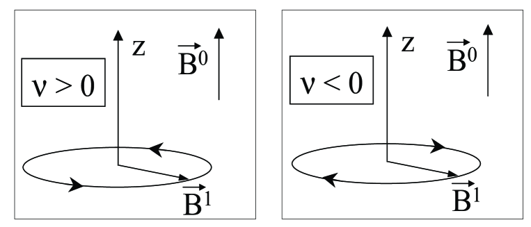
Figure 2: Different kinds of polarization of the electromagnetic wave for $\nu>0$ and $\nu<0$.

IV.1 Scheme for numerical simulations

The numerical simulations are performed without using the perturbation approach and results are presented in Sec. VI below. It is convenient to work in the rotating frame where the effective Hamiltonian is independent of time. The relationship between the wave function $|\Psi(t)\rangle$ in the laboratory frame and the wave function $|\Phi(t)\rangle$ in the rotating frame is

$$|\Psi(t)\rangle=e^{i\hat{\Sigma}(\nu t+\varphi)}|\Phi(t)\rangle.$$ (36)

The Schrödinger equation in the rotating frame is

$$i|\dot{\Phi}(t)\rangle=\left(\hat{H}^{0}+\nu\hat{\Sigma}+\hat{V}\right)|\Phi(t)\rangle,$$ (37)

$$\hat{V}=\Omega_{e}(\hat{S}^{x}_{1}+\hat{S}^{x}_{2})-\Omega_{n}^{0}(\hat{I}^{x}_{1}+\hat{I}^{x}_{2}).$$ (38)

Let us decompose the wave function over the eigenstates $|\psi_{n}\rangle$ of the Hamiltonian $\hat{H}_{0}$ as

$$|\Phi(t)\rangle=\sum_{n=0}^{15}c_{n}(t)|\psi_{n}\rangle,$$ (39)

where the functions $|\psi_{n}\rangle$ are related to the basis functions $|i\rangle$ by

$$|\psi_{n}\rangle=\sum_{i}a_{n,i}|i\rangle.$$ (40)

The coefficients $a_{n,i}$ are calculated in Section II in the zeroth order approximation. (For our numerical simulations we use the exact values of $a_{n,i}$.) The system of 16 differential equations for the expansion coefficients $c_{n}(t)$ is

$$i\dot{c}_{n}(t)=\left(E_{n}+\Sigma_{n}\nu\right)c_{n}(t)+\sum_{m=0}^{15}V_{nm}c_{m}(t),$$ (41)

where

$$V_{n,m}=\langle\psi_{n}|\hat{V}|\psi_{m}\rangle.$$ (42)

Eq. (41) can be regarded as the Schrödinger equation

$$i\dot{c}_{n}(t)=\sum_{m=0}^{15}h_{n,m}c_{m}(t)$$ (43)

with the time-independent Hamiltonian $\hat{h}$ whose matrix elements have the following form:

$$h_{n,m}=(E_{n}+\nu\Sigma_{n})\delta_{nm}+V_{nm}.$$ (44)

The dynamics of the coefficients $c_{n}(t)$ can be computed using the eigenfunctions $b^{q}_{n}$, $q=0,\dots,15$ and the eigenvalues $e^{q}$ of the Hamiltonian $\hat{h}$ as

$$c_{n}(t)=\sum_{m=0}^{15}c_{m}(t_{0})\sum_{q=0}^{15}\left(b^{q}_{m}\right)^{*}b^{q}_{n}e^{-ie^{q}(t-t^{\prime})},$$ (45)

where $t^{\prime}$ is the time of the beginning of the pulse. The wave function in the laboratory frame can be represented as

$$|\Psi(t)\rangle=\sum_{p=0}^{15}D_{p}(t)e^{-iE_{p}t}|\psi_{p}\rangle.$$ (46)

Before each pulse at time $t=t^{\prime}$ we make the transformation to the rotating frame using the relation [see Eqs. (36), (39) and (46)]

$$D_{p}(t)=\exp\left[iE_{p}t+i\Sigma_{p}(\nu t+\varphi)\right]c_{p}(t),$$ (47)

and after the pulse at the time $t=t^{\prime}+\tau$ ($\tau$ is the duration of the pulse) we make the back transformation to the laboratory frame using the same formula.

V Implementation of logic gates

We describe here implementation of logic gates in terms of the basis states $|i\rangle$, $i=0,\dots,15$. From Section II the basis functions $|i\rangle$ are approximately equal to the eigenfunctions $|\psi_{i}\rangle$ if the conditions $\gamma_{e}\delta B\gg J/2$ and $|\gamma_{e}\delta B-A/2|\gg J/2$ are satisfied. Assume that the frequency of a pulse is close to the transition frequency of the $k$th ($k=1,2$) electron or nuclear spin; the direction of the spin in the state $|p\rangle$ is along the direction of the permanent magnetic field $\vec{B}^{0}$ (i.e. $|p\rangle=|\dots\uparrow_{k}\dots\rangle$ or $|p\rangle=|\dots\Uparrow_{k}\dots\rangle$); and the state $|q\rangle$ is related to the state $|p\rangle$ by a flip of the $k$th spin. For the initial conditions

$$D_{p}(t^{\prime})=1,\qquad D_{q}(t^{\prime})=0$$

the dynamics of this spin is described by the following equations book ; book1 :

$$D_{p}(t^{\prime}+\tau)=\left\{\cos\left[{\lambda_{q,p}\tau\over 2}\right]+i{\Delta_{q,p}\over\lambda_{q,p}}\sin\left[{\lambda_{q,p}\tau\over 2}\right]\right\}e^{-i\Delta_{q,p}\tau/2},$$

$$D_{q}(t^{\prime}+\tau)=i{\Omega\over\lambda_{q,p}}\sin\left[{\lambda_{q,p}\tau\over 2}\right]e^{i\Delta_{q,p}t^{\prime}-i\varphi+i\Delta_{q,p}\tau/2},$$ (48)

where

$$\Delta_{q,p}=E_{q}-E_{p}-\nu,~{}~{}\lambda_{q,p}=\sqrt{\Delta^{2}_{q,p}+\Omega^{2}},$$

$t^{\prime}$ is the time of the beginning of the pulse, $\tau$ is the duration of the pulse, $\Omega=\Omega_{e}$ is the Rabi frequency of the electron spin, and $\Omega=\Omega_{n}$ is the Rabi frequency of the nuclear spin. For the other initial conditions

$$D_{p}(t^{\prime})=0,\qquad D_{q}(t^{\prime})=1$$

the solution is

$$D_{p}(t^{\prime}+\tau)=i{\Omega\over\lambda_{q,p}}\sin\left[{\lambda_{q,p}\tau\over 2}\right]e^{-i\Delta_{q,p}t^{\prime}+i\varphi-i\Delta_{q,p}\tau/2},$$

$$D_{q}(t^{\prime}+\tau)=\left\{\cos\left[{\lambda_{q,p}\tau\over 2}\right]-i{\Delta_{q,p}\over\lambda_{q,p}}\sin\left[{\lambda_{q,p}\tau\over 2}\right]\right\}e^{i\Delta_{q,p}\tau/2}.$$ (49)

The complete transition between the states $|p\rangle$ and $|q\rangle$ takes place when the detuning is equal to $\Delta_{q,p}=0$ and when $\tau=\pi/\Omega$ ($\pi$-pulse). A near-resonant transition with $\Delta\neq 0$ can be completely suppressed when the condition book

$$\Omega={|\Delta_{q,p}|\over\sqrt{4K^{2}-1}},$$ (50)

known as the $2\pi K$ condition, is satisfied. Here $K=1,2,\dots$ is an integer number. For this value of $\Omega$ the value of the sine in Eqs. (48) and (49) is equal to zero.

As follows from the above considerations, (i) in order to implement a complete transition, the frequency of the pulse must be resonant to this transition, $\nu=E_{q}-E_{p}$, where $\nu$ can assume both positive and negative values. (ii) In order to completely suppress a transition with $\Delta\neq 0$, the Rabi frequency of the pulse must satisfy the $2\pi K$-condition (50). Both operations (i) and (ii) can be implemented simultaneously by one pulse if there are two states in the quantum register. Actually, we described here the procedure for implementation of the Control-Not gate, which we will use to create entanglement in our system.

We now derive the parameters of the gates described in Section III. Let CN_l,k be the Control-Not gate which flips the $k$th spin in the state $|i\rangle$ and suppresses the flip of the same spin in the state $|j\rangle$ (the latter has different orientation of the $l$th spin). We assume that the $k$th spin is pointed up (along the direction of $\vec{B}^{0}$) in both states $|i\rangle$ and $|j\rangle$. Let the state $|i^{\prime}\rangle$ be related to the state $|i\rangle$ by the flip of the $k$th spin and the state $|j^{\prime}\rangle$ be related to the state $|j\rangle$ by the flip of the same spin. Then the frequency $\nu$ and the detuning $\Delta_{j^{\prime},j}$ in Eq. (50) for the Rabi frequency are

$$\nu=E_{i^{\prime}}-E_{i},~{}~{}~{}\Delta_{j^{\prime},j}=E_{j^{\prime}}-E_{j}-\nu.$$ (51)

In our notation, it is convenient to treat the state of the electron spin $|\Uparrow_{k}\rangle$ as $|0_{k}\rangle$ and the state $|\Downarrow_{k}\rangle$ as $|1_{k}\rangle$. The fact that the energy of the state $|0_{k}\rangle$ is larger than the energy of the state $|1_{k}\rangle$ is accounted for by a negative frequency $\nu$ of the pulse in the first equation (51) .

V.1 Initialization

The nuclear spins can be polarized by using the fact that the Larmor frequencies of the electron spins depend on orientations of the corresponding nuclear spins through the hyperfine interaction. Measuring the electron Larmor frequencies using, for example, a scanning tunneling microscope init1 ; init2 , one can define the orientation of the nuclear spins and apply a selective $\pi$-pulse if necessary. Here we describe a different technique. We assume that initially the nuclear spins are not polarized, the electron spins are polarized, and there are four states (32) in the register. If we apply the gates

$${\rm CN}_{e_{1},n_{1}}{\rm CN}_{n_{1},e_{1}}$$ (52)

(the order of implementation of the operators is from the right to the left), we obtain the superposition of states

$$|n_{2}\Downarrow_{2}\,e_{1}\downarrow_{1}\,\rangle$$ (53)

with indefinite orientation of the first electron spin and with definite orientation of the first nuclear spin.

Since the state of the first electron spin in Eq. (53) is unknown, we cannot immediately swap the states of the second electron and nuclear spins because of the interaction between the electron spins. One has to wait while the electron spin polarizes again (during, for example, the time-interval 0.1 s). In our numerical simulations the relaxation of the electron spins is modeled by flipping them “by hand”, without using electromagnetic pulses, in all states of superposition.

After the electron spins are polarized one applies the gates

$${\rm CN}_{e_{2},n_{2}}{\rm CN}_{n_{2},e_{2}}$$ (54)

and obtains the state

$$|\downarrow_{2}\,e_{2}\Downarrow_{1}\,\downarrow_{1}\,\rangle.$$ (55)

One waits while the second electron spin relaxes and obtains the state

$$|\downarrow_{2}\,\Downarrow_{2}\,\Downarrow_{1}\,\downarrow_{1}\,\rangle$$ (56)

which is used as an initial state for creation of the entanglement.

V.2 Entanglement

The sequence of gates

$$\overline{{\rm CN}}_{e_{2},n_{2}}\overline{{\rm CN}}_{e_{1},e_{2}}\overline{{\rm CN}}_{n_{1},e_{1}}{\rm Had}_{n_{1}}$$ (57)

generates the entangled state (33). In Eq. (57) ${\rm Had}_{n_{1}}$ is the Hadamard gate on the first nuclear spin, and the gate $\overline{{\rm CN}}_{k,k^{\prime}}$ is the inverse of the Control-Not gate: it flips the target qubit only if the control qubit is in the state $|0_{k}\rangle$. The parameters of these gates can be calculated analytically using Eq. (51). In our simulations presented below, the Hadamard gate is performed by applying a $\pi/2$ pulse of duration $\tau=\pi/(2\Omega_{n})$, where $\Omega_{n}$ is given by Eq. (76) below.

In principle, it is possible to inplement a Control-Not gate between the nuclear spins without changing the states of the electron spins adiabatic1 . In practice, this approach is not useful because one can show (using calculated in this paper eigenvalues) that the mediated by the electrons effective coupling between the nuclear spins is of the order of 3.5 Hz or less. This means that the Rabi frequency of the pulse implementing the Control-Not gate must be less than 2 Hz and the frequency of the pulse must be tuned in resonance with the accuracy of approximately 0.1 Hz.

V.3 Rabi frequencies

The Rabi frequency of the electron spins $\Omega_{e}$ is different from $\Omega_{e}^{0}=\gamma_{e}B^{1}$ because of the exchange interaction between the electron spins. Similarly, the Rabi frequency of the nuclear spins $\Omega_{n}$ is different from $\Omega_{n}^{0}=\gamma_{n}B^{1}$ because of the hyperfine interaction between the nuclear and electron spins.

Consider, for example, the transition

$$|\uparrow_{2}\,\Downarrow_{2}\,\Downarrow_{1}\,\uparrow_{1}\,\rangle\rightarrow|\uparrow_{2}\,\Downarrow_{2}\,\Uparrow_{1}\,\uparrow_{1}\,\rangle,$$ (58)

associated with the flip of the first electron spin. The matrix element $V_{6,4}=\Omega_{e}/2$ of the matrix $h_{n,m}$ in Eq. (44) is responsible for this transition. The value of $\Omega_{e}$ must satisfy the $2\pi K$ condition (50). The value of $V_{6,4}$ can be calculated using Eq. (42). Only two terms in the sum

$$V_{nm}=\sum_{i,j=0}^{15}a_{i,n}\langle i|\hat{V}|j\rangle a_{m,j},$$ (59)

where $n=6,~{}m=4$, appreciably contribute. These are

$$V_{6,4}=\sum_{i,j=0}^{15}a_{i,6}\langle i|\hat{V}|j\rangle a_{4,j}\approx a_{6,6}\langle 6|\hat{V}|4\rangle a_{4,4}+a_{6,6}\langle 6|\hat{V}|2\rangle a_{4,2}.$$ (60)

The first term is due to the flip of the first electron spin by the electromagnetic pulse, i.e., due to the transition

$$|\uparrow_{2}\,\Downarrow_{2}\,\Downarrow_{1}\,\uparrow_{1}\,\rangle\rightarrow|\uparrow_{2}\,\Downarrow_{2}\,\Uparrow_{1}\,\uparrow_{1}\,\rangle,$$ (61)

The second term is due to the two-step transition

$$|\uparrow_{2}\,\Downarrow_{2}\,\Downarrow_{1}\,\uparrow_{1}\,\rangle\rightarrow|\uparrow_{2}\,\Uparrow_{2}\,\Downarrow_{1}\,\uparrow_{1}\,\rangle\rightarrow|\uparrow_{2}\,\Downarrow_{2}\,\Uparrow_{1}\,\uparrow_{1}\,\rangle,$$ (62)

where the first step is due to the nonselective excitation of the second electron spin and the second step is implemented due to the exchange interaction between the electrons. The contribution of the second term is proportional to the ratio of the matrix element $J/2$, responsible for the exchange interaction, [see the second transition in Eq. (62)] to the detuning $2\delta B$, characterizing the first transition. From Eq. (60) the Rabi frequency is

$$\Omega_{e}\approx\Omega_{e}^{0}\left(1-{J\over 4\gamma_{e}\delta B}\right).$$ (63)

This expression for the electron Rabi frequency holds for all other electron transitions. The $2\pi K$ condition (50) for the electron spin becomes

$$\Omega^{0}_{e}=\gamma_{e}B^{1}={|\Delta_{j^{\prime},j}|\over\sqrt{4K_{e}^{2}-1}}\left(1-{J\over 4\gamma_{e}\delta B}\right)^{-1},$$ (64)

where $|\Delta_{j^{\prime},j}|\approx A$ when the control spin is the nuclear spin and $|\Delta_{j^{\prime},j}|\approx J$ when the control spin is the neighboring electron spin.

We now find the Rabi frequency of the nuclear spin. Consider the gate ${\rm CN}_{e_{1},n_{1}}$ in Eq. (52) acting on the state $|\uparrow_{2}\,\Downarrow_{2}\,\Downarrow_{1}\,\uparrow_{1}\,\rangle$. The nuclear spin is flipped as a result of the transition

$$|\uparrow_{2}\,\Downarrow_{2}\,\Downarrow_{1}\,\uparrow_{1}\,\rangle\rightarrow|\uparrow_{2}\,\Downarrow_{2}\,\Downarrow_{1}\,\downarrow_{1}\,\rangle,$$ (65)

which is implemented through the matrix element $V_{6,7}=-\Omega_{n}/2$. In Eq. (42), only two terms considerably contribute to the value of $V_{6,7}$, namely

$$V_{6,7}\approx a_{6,6}\left(-{\Omega_{n}^{0}\over 2}\right)a_{7,7}+a_{5,6}{\Omega_{e}^{0}\over 2}a_{7,7}.$$ (66)

The first term is due to the flip of the nuclear spin by the electromagnetic pulse in Eq. (65). The second term is due to the two-step transition

$$|\uparrow_{2}\,\Downarrow_{2}\,\Downarrow_{1}\,\uparrow_{1}\,\rangle\rightarrow|\uparrow_{2}\,\Downarrow_{2}\,\Uparrow_{1}\,\downarrow_{1}\,\rangle\rightarrow|\uparrow_{2}\,\Downarrow_{2}\,\Downarrow_{1}\,\downarrow_{1}\,\rangle,$$ (67)

where the first step is due to the hyperfine interaction between the first electron spin and the first nuclear spin and the second step is due to the nonresonant action of the electromagnetic pulse on the first electron spin. The transition (67) is initiated by the electron spin, which creates a magnetic field in the $x$ direction comparable to the magnetic field $B^{1}$ of the pulse. In spite of the fact that the probability $P_{e}$ of flipping the electron spin is small, the fact that $\Omega_{e}/\Omega_{n}^{0}\sim 10^{3}$ makes the probability of the transition (67) comparable to the probability of the transition (65).

In order to calculate $a_{5,6}$ in Eq. (66), we must calculate the first-order correction to the wave function (26) using the equation

$$|\psi_{n}^{(1)}\rangle=\sum_{m=0\atop m\neq n}^{15}{V_{n,m}\over E^{(0)}_{m}-E^{(0)}_{n}}|\psi_{m}^{(0)}\rangle.$$ (68)

Taking $n=5$ and multiplying by $\langle 6|$ we obtain

$$a_{5,6}=\sum_{m=0\atop m\neq 5}^{15}{V_{5,m}a_{m,6}\over E^{(0)}_{m}-E^{(0)}_{5}}.$$ (69)

Only one term with $m=6$ significantly contributes to the sum, where

$$V_{5,6}\approx\langle 5|\hat{V}|6\rangle={A\over 2}.$$

We find

$$a_{5,6}\approx{A\over 2[E^{(0)}_{6}-E^{(0)}_{5}]}\approx-{A\over 2\gamma_{e}b}\ll 1.$$

Putting this value to Eq. (66) we obtain the expression for the Rabi frequency of the nucleus

$$\Omega_{n}=\Omega_{n}^{0}+{A\over 2\gamma_{e}b}\Omega_{e}^{0}\approx 2\Omega_{n}^{0}.$$ (70)

This equation is valid for the Rabi frequencies associated with other nuclear spin transitions. Similar to Eq. (63) for the electron spin, the correction to the Rabi frequency is proportional to the ratio of the matrix element $A/2$, responsible for the hyperfine interaction, to the detuning $\gamma_{e}b\approx\gamma_{e}b-\gamma_{n}b$ between the frequencies of the nuclear and electron spins.

The $2\pi K$ condition for the nuclear spin reads

$$\Omega^{0}_{n}=\gamma_{n}B^{1}={|\Delta_{j^{\prime},j}|\over\sqrt{4K_{n}^{2}-1}}\left(1+{A\over 2\gamma_{n}b}\right)^{-1},$$ (71)

where $|\Delta_{j^{\prime},j}|\approx A$. We have calculated the Rabi frequencies only for the two gates. The Rabi frequencies for the other gates can be calculated using the same formulas (64) and (71).

We still have indefinite parameters $K_{e}$ and $K_{n}$ in Eqs. (64) and (71) for the Rabi frequencies of electron and nuclear spins. Increasing $K_{e}$ and $K_{n}$ decrease the electron and nuclear Rabi frequencies which should satisfy the conditions

$$\varepsilon_{e}={\Omega_{e}\over 4\gamma_{e}\delta B}\ll 1,~{}~{}~{}\varepsilon_{n}={\Omega_{n}\over 4\gamma_{n}\delta B}\ll 1.$$ (72)

These conditions provide selective excitations of the spins nonresonant . The error in the probability amplitude due to nonselective excitations is of the order of $\varepsilon_{e}$ for the electron spins and of the order of $\varepsilon_{n}$ for the nuclear spins. The condition (72) can be written as $B^{1}/(4\delta B)\ll 1$. If the distance between the qubits is 10 nm and the magnetic field gradient is $10^{5}$ T/m gradient1 ; gradient2 ; gradient3 , then $B^{1}\ll 4\delta B=2\times 10^{-3}$ T. Hence,

$${\Omega_{e}\over 2\pi}\approx{\gamma_{e}\over 2\pi}B^{1}\ll 56{\rm MHz},$$ (73)

We now choose $K=K_{e}$ for the electron spin to satisfy the following two conditions: (i) The value of $K_{e}$ must be large enough to satisfy the first equation (72), which allows one to decrease the error due to nonselective excitations; (ii) and the time $\tau_{e}$ of implementation of the Control Not gate on the (target) electron spin must be much smaller than the electron relaxation time $T_{c}$ (we assume $T_{c}=60$ ms T_c ). This condition can be satisfied by decreasing $K_{e}$.

Consider the Control-Not gate on the electron spin with control nuclear spin. The error $\sqrt{P_{e}}$ due to nonselective excitation of the electron spins is of the order of [for $|\Delta|\approx A$ in Eq. (50)]

$$\sqrt{P_{e}}\sim{\Omega_{e}\over 4\gamma_{e}\delta B}\approx{A\over 8\gamma_{e}\delta BK_{e}}\approx{1.03\over K_{e}},$$ (74)

where we used the parameters $A/2\pi=116$ MHz, the magnetic field gradient $10^{5}$ T/m, and the distance 10 nm. In our simulations we take $K_{e}=103$ so that the error is $\sqrt{P_{e}}\approx 0.01$. The Rabi frequency and the time duration of the $\pi$-pulse are

$${\Omega_{e}\over 2\pi}\approx{A\over 2\pi\sqrt{4K_{e}^{2}-1}}\approx 563~{}{\rm kHz},~{}~{}~{}\tau_{e}\approx 0.89~{}\mu{\rm s}.$$

Consider the Control-Not gate on the electron spin with control electron spin. The error is of the order of ($|\Delta|\approx J$) $\sqrt{P_{e}^{\prime}}\sim 0.01$ if $K_{e}^{\prime}=1$, where we assume $J/(2\pi)=500$ kHz. The Rabi frequency and the time duration of the $\pi$-pulse are

$${\Omega_{e}^{\prime}\over 2\pi}\approx{J\over 2\pi\sqrt{4{K_{e}^{\prime 2}-1}}}\approx 289~{}{\rm kHz},~{}~{}~{}\tau_{e}^{\prime}=2~{}\mu{\rm s}.$$

Due to the second equation (72), the Rabi frequency $\Omega_{n}$ must satisfy the condition

$${\Omega_{n}\over 2\pi}\approx{2\gamma_{n}\over 2\pi}B^{1}\ll 34.5{\rm kHz}.$$ (75)

For implementation of the Control Not gate, $\Omega_{n}$ must also satisfy the $2\pi K$ condition (71). The error in the Control-Not gate on the nuclear spin with control electron spin is $\sqrt{P_{n}}\sim 0.05$ if $K=K_{n}=33,620$. The Rabi frequency and the time duration of the $\pi$-pulse acting on a nuclear spin are

$${\Omega_{n}\over 2\pi}\approx{A\over 2\pi\sqrt{4{K_{n}^{2}-1}}}\approx 1.7~{}{\rm kHz},~{}~{}~{}\tau_{n}\approx 0.3~{}{\rm ms}.$$ (76)

We note here that the magnetic field gradient practically defines the clock speed of our quantum computer. During the time of implementation of the Control Not gate on the nuclear (target) spin, the electron (control) spin must stay coherent so that the condition $\tau_{n}\ll T_{c}$, where $T_{c}$ is the transverse relaxation time, must be satisfied. For isotopically purified ²⁸Si, the relaxation time $T_{c}$ can be as long as $60$ ms T_c at 7 K, which is large enough for implementation of the Control-Not gate. In natural Si (4.7% of ²⁹Si) the value of $T_{c}$ is smaller than 0.6 ms at 1.6 K T_c , which is too small for implementation of the Control-Not gate on the nuclear spin. The Rabi frequency of the order of 1.7 kHz is large in comparison to the dipole-dipole interaction between the electron and nucleus of the neighboring phosphorus atoms, which is close to 32 Hz for the distance 10 nm between the qubits, so that one can neglect this dipole-dipole interaction.

We now make some comments about precision of calculation of the energy levels in Section II. As follows from Eqs. (48) and (49), the spin rotates around the $x$ axis (in the rotating frame) with the frequency

$$\lambda_{q,p}=\sqrt{\Delta_{q,p}^{2}+\Omega^{2}}.$$ (77)

If we wish to implement the resonant transition, $\Delta_{q,p}$ must be equal to zero. Since $\Delta_{q,p}=E_{q}-E_{p}-\nu$ is defined by the distance between the energy levels (eigenvalues), the complete transition takes place only if these eigenvalues are exactly known. For a system with a small number of qubits, the eigenvalues can be calculated numerically with a high precision. For a system with a large number of qubits, ($>30$) one can use the perturbation theory described in Section II. This theory allows one to calculate the eigenvalues with precision $\epsilon^{m}A/2$, where $\epsilon$ is defined in Eq. (6) and $m$ is the order of the perturbation theory ($m=2$ in our paper and $m=1$ for the zeroth order approximation). The limited accuracy of $E_{q}$ and $E_{p}$ results in a finite detuning of the order of

$$|\Delta_{q,p}|\sim\epsilon^{m}{A\over 2}.$$

In order for this detuning to have a small influence on the dynamics, the value of $|\Delta_{q,p}|$ in Eq. (77) must be much smaller than the value of $\Omega$. From Eq. (6) we have $\epsilon=6\times 10^{-4}$. In the zeroth order approximation ($m=1$), the value of $|\Delta_{q,p}/(2\pi)|$ is of the order of 35 kHz, which is much larger than $\Omega_{n}/(2\pi)$ in Eq. (76) and is not acceptable. In the second order approximation ($m=2$), we have $|\Delta_{q,p}/(2\pi)|\sim 21$ Hz, which is much smaller than $\Omega_{n}/(2\pi)$ so that this is an acceptable approximation for us. In practice, the above argument means that the frequency $\nu$ of the electromagnetic wave must be tuned with an accuracy of the order of several tens of Hertz in order to flip a nuclear spin without generating a substantial error.

V.4 Spin relaxation

The relaxation of the electron spin can affect (flip) the nuclear spin via the hyperfine interaction. Here we discuss the conditions required to suppress the nuclear spin flip during the electron spin relaxation process. Other kinds of relaxation mechanisms can be neglected because the relaxation time $T_{n}$ of a neutron is at least four order of magnitude larger ($T_{n}\sim 3\times 10^{3}$ s relaxN ) than the total time of implementation of the algorithm. The electron spin relaxation allows us to implement the nonunitary transformation

$$\begin{array}[]{lll}D_{0}|\Uparrow\downarrow\rangle&\rightarrow&|\Downarrow\downarrow\rangle\\ &\nearrow&\\ D_{1}|\Downarrow\downarrow\rangle&&,\end{array}$$ (78)

which is necessary for creation of the initial state.

Consider the dynamics of the classical nuclear magnetic moment $\vec{I}(t)$ placed in a permanent external field $\vec{B}^{0}$ oriented along the z axis and a field created by the electron spin $\vec{S}(t)$. Here the $z$ component $S^{z}(t)$ of the electron spin is a given function of time $t$. The slowly varying $z$ component of the magnetic field acting on the nuclear spin is

$$B^{z}(t)=B^{0}-{A\over\gamma_{n}\hbar}S^{z}(t).$$ (79)

The electron spin rotates with the frequency $\gamma_{e}B^{0}$ and generates a circularly polarized time-dependent magnetic field acting on the nuclear spin via the hyperfine interaction. Since $\gamma_{e}B^{0}$ is three orders of magnitude larger than the Larmor frequency of the nuclear spin, this fast field does not affect the dynamics of the nuclear spin because the nuclear spin is out of resonance with the field generated by the fast-rotating electron spin.

There are always stray magnetic fields in a real system, such as, for example, the Earth’s field, which can affect the dynamics of the nuclear spin. Without loss of generality, we assume that this field, $B^{x}$, is oriented along the $x$ axis. The nuclear spin is flipped if two conditions are satisfied. (a) The $B^{z}$ field (79) must go through the zero point $B^{z}(t)=0$. (b) The condition of adiabatic passage adiabatic

$$\xi={\left|\dot{B}^{z}\right|\over\gamma_{n}\left(B^{x}\right)^{2}}\ll 1$$ (80)

must hold. Here $\xi$ is a dimensionless small parameter. We now analyze how to choose the parameters of our system in order to violate these two conditions and, thus, to suppress the nuclear spin flip.

Condition (a) is satisfied if the value of $B^{z}$ in Eq. (79) is always positive, which yields the minimum value $B^{0}_{\rm min}$ of the external field (for $S^{z}=1/2$)

$$B^{0}>B^{0}_{\rm min}={A\over 2\gamma_{n}\hbar}\approx 3.36~{}{\rm T}.$$ (81)

Even if condition (a) is not satisfied, the nuclear spin cannot flip if the magnetic field $B^{x}$ is sufficiently small to violate condition (b). With a good approximation the function $S^{z}(t)$ can be chosen in the form Gorshkov

$$S^{z}(t)={1\over 2}\left(1-2{t\over T_{c}}\right).$$ (82)

The parameter $\xi$ in Eq. (80) becomes

$$\xi\approx{6.2\times 10^{3}\over\tilde{T}_{c}\left(\tilde{B}^{x}\right)^{2}},$$ (83)

where the dimensionless relaxation time $\tilde{T}_{c}$ is equal to the number of milliseconds [$\tilde{T}_{c}=T_{c}/(1~{}{\rm ms})$] and the dimensionless $B^{x}$ field $\tilde{B}^{x}$ is equal to the number of gauss [$\tilde{B}^{x}=B^{x}/(1~{}{\rm gauss})$]. We take $\tilde{T}_{c}=6$ (so that $T_{c}=6$ ms). If $B^{x}$ is equal to the Earth’s magnetic field, $\tilde{B}^{x}=0.5$, the condition of adiabatic passage is not satisfied, $\xi\approx 4.1\times 10^{3}\gg 1$ so that the nuclear spin does not flip. The numerical modeling of the classical spin dynamics with $B^{x}=0.5~{}{\rm gauss}$ and

$$B^{0}=3.3T<B^{0}_{\rm min},~{}~{}~{}T_{c}=6~{}{\rm ms},~{}~{}~{}I^{z}(t=0)=-0.5$$ (84)

yields

$$\delta I^{z}={I^{z}(0)-I^{z}(T_{c})\over I^{z}(0)}\approx 7.5\times 10^{-4}.$$

One can show that the error in the quantum probability amplitude is of the order of $\delta I^{z}$. One can neglect this error if it is small in comparison with the other errors. For $B^{x}=5~{}{\rm gauss}$ we have $\xi\approx 41$, and a numerical simulation gives $\delta I^{z}\approx 0.075$. For $B^{x}=50~{}{\rm gauss}$ we have $\xi\approx 0.41$ and numerical simulations show that the nuclear spin flips and $I^{z}(T_{c})\approx 0.5$. This is the situation when the conditions of adiabatic passage are satisfied which prevent the initialization of our computer.

If the transverse magnetic field is relatively strong, for example, when $B^{x}=50~{}{\rm gauss}$, one can suppress the flip of the nuclear spin by violating condition (a). For example, increasing $B^{0}$ from $B^{0}=3.3$ T, which is less than $B^{0}_{\rm min}$ in Eq. (81), to $B^{0}=3.5~{}\rm{T}>B^{0}_{\rm min}$ and for the same transverse magnetic field $B^{x}=50~{}{\rm gauss}$, we numerically obtained $\delta I^{z}(T_{c})=7\times 10^{-4}$, i.e. the nuclear spin actually does not flip.

Next we will show that, in the situation when the conditions of adiabatic passage are satisfied for certain spins, the error still can be small if $B^{0}$ is close to $B^{0}_{\rm min}$, i.e. when $|(B^{0}_{\rm min}-B^{0})/B^{0}_{\rm min}|\ll 1$. Assume that we are dealing with an ensemble of identical spin chains as mentioned in the introduction, $B^{0}<B^{0}_{\rm min}$, and condition of adiabatic passage (80) is satisfied. Since before the relaxation the electron spins point in a random direction, not all of them pass the point for which $B^{z}(t)=0$ in Eq. (79). In Fig. 3 we show how the magnetic field acting on different nuclear spins changes with time. Only those nuclear spins flip for which the condition

$$B^{0}-{A\over 2\gamma_{n}\hbar}S^{z}(0)\leq 0$$

holds. As follows from the figure, the total number of such spins in the ensemble is

$$\eta={d\over d+d^{\prime}}=\frac{1}{2}-{\gamma_{n}B^{0}\hbar\over A}=\frac{1}{2}\left(1-{B^{0}\over B^{0}_{\rm min}}\right).$$ (85)

The error $\sqrt{P_{\rm r}}$ in the probability amplitude for the ensemble is $\sqrt{P_{\rm r}}\approx\eta$. For example, for $B^{0}=3.3$ T (and for $B^{0}_{\rm min}=3.36$ T) we have $\eta=0.009$ which is a small error. In summary, our analysis shows that it is possible to suppress the flip of the nuclear spin during the relaxation of the electron spin and to implement the transformation (78).

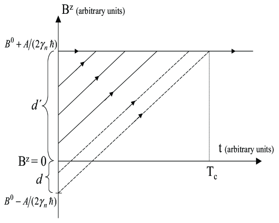
Figure 3: A schematic illustration of the magnetic field acting on the nuclear spin for different values of $S^{z}(0)$ [$S^{z}(0)=1/2$ for the lowest curve and $S^{z}(0)=-1/2$ for the top curve]. The nuclear spin flips for the magnetic fields illustrated by the dashed curves and does not flip for the magnetic fields shown by the solid curves.

VI Numerical results

In our four-qubit system, all parameters of the pulses can be calculated numerically using exact eigenvalues of the matrix $\hat{H}^{0}$ and off-diagonal elements of the matrix $\hat{V}$, which are equal to $\Omega_{e}/2$ for electron transitions and $-\Omega_{n}/2$ for the nuclear transitions. In spite of the ability to calculate the parameters numerically, we calculate them analytically using our perturbative approach and simulate the quantum dynamics numerically as described in Sec. IV.1. Our analysis has the following advantages: (i) it can be applied to a system with an arbitrary number of qubits (ii) it allows one to take into consideration only “slow” transitions with small detunings and to neglect fast transitions with relatively large detunings, which have little influence the quantum dynamics. Using our approach it is possible to understand the most important sources of error and to minimize them by the optimal choice of pulse parameters.

We start with the state

$$|\Psi(0)\rangle=C_{6}(0)|6\rangle+C_{7}(0)|7\rangle+C_{14}(0)|14\rangle+C_{15}(0)|15\rangle$$ (86)

with arbitrarily chosen complex coefficients $C_{6}(0)$, $C_{7}(0)$, $C_{14}(0)$, and $C_{15}(0)$ at time $t=0$. Then we make the transformation to the representation of the Hamiltonian $\hat{H}^{0}$ [see Eq. (40)]

$$D_{n}(0)=\sum_{i=0}^{15}a_{n,i}C_{i}(0).$$ (87)

After initialization of the system and creation of entanglement, we make the back transformation

$$C_{i}(T)=\sum_{n=0}^{15}a_{i,n}D_{n}(T)e^{-iE_{n}T},$$ (88)

where $T$ is the total time of implementation of the protocol. The error is calculated as

$$P=\left|{1\over 2}-|C_{0}(T)|^{2}\right|+\left|{1\over 2}-|C_{15}(T)|^{2}\right|.$$ (89)

Figure 4: The probability error $P$ as a function of $J/(2\pi)$; $\delta B=0.5$ mT.

In Fig. 4 we plot the error after implementation of initialization and entanglement. Each point on the plot is the average over 100 realizations with randomly chosen complex coefficients $C_{6}(0)$, $C_{7}(0)$, $C_{14}(0)$, and $C_{15}(0)$. One can see that the error increases with $J$ increasing. When $J$ is large enough, $J\sim 4\gamma_{e}\delta B$, the basis states $|n\rangle$ differ considerably from the eigenstates $|\psi_{n}\rangle$ of the Hamiltonian $\hat{H}^{0}$, so that the error is generated as a result of free evolution of the basis states. The error bars are the consequence of the fact that the protocol processes some initial states of the superposition better than other states.

Figure 5: The probability error $P$ as a function of magnetic field difference 2$\delta B$ for $J/(2\pi)=2$ MHz. The data are averaged over 100 realizations with randomly chosen normalized complex coefficients $C_{6}(0)$, $C_{7}(0)$, $C_{14}(0)$, and $C_{15}(0)$.

In Fig. 5 we plot the probability error $P$ as a function of the magnetic field difference $2\delta B=B_{2}^{z}-B_{1}^{z}$ for the interval $0.1~{}{\rm mT}\leq 2\delta B\leq 5~{}{\rm mT}$. For a qubit spacing of 10 nm, this interval corresponds to magnetic field gradients from $10^{-4}$ to $5\times 10^{-5}$ T/m. As follows from the figure, the error is large when $2\delta B$ is small, i.e. when $J/(4\gamma_{e}\delta B)\sim 1$.

The maximum in $P$ near $2\delta B\approx 4.2$ mT is defined by the condition $\gamma_{e}\delta B=A/2$. When this condition is satisfied the 10th and 12th eigenvectors defined in Eq. (28) and (30) become symmetric and antisymmetric superpositions

$$|\downarrow_{2}\,\rangle\otimes\left[{1\over\sqrt{2}}\left(|\Downarrow_{2}\,\Uparrow_{1}\,\rangle\pm|\Uparrow_{2}\,\Downarrow_{1}\,\rangle\right)\right]\otimes|\uparrow_{1}\,\rangle.$$

These states are formed because the electron frequency difference caused by the magnetic field gradient is compensated by the hyperfine interactions between the electrons and nuclei.

The numerical results indicate that it is worthwhile to place neighboring qubits at larger distance $d$ from each other. This gives one the following advantages. (i) At a given gradient, the value of $\delta B=(B^{2}_{z}-B^{1}_{z})/2$ increases with increasing $d$, which provides better selectivity of the pulses and increases the clock speed of the quantum computer [see the second equation (72) and Eq. (76)]. (ii) The value of $J$ decreases with increasing $d$  sarma . This does not affect the clock speed of the quantum computer because the clock speed is defined by $\delta B$. (iii) Decreasing $J$ decreases the influence of the off-diagonal components of the exchange interaction and the eigenstates $|\psi_{n}\rangle$ of the Hamiltonian $\hat{H}^{0}$ are better approximated by the basis states $|n\rangle$. Since $|\psi_{n}\rangle\neq|n\rangle$, the error in the probability amplitude [proportional to $J/(4\gamma_{e}\delta B$)] is generated even in the stationary system when no electromagnetic pulses are applied. (iv) In a system with more than two qubits increasing $d$ decreases unwanted effect of long-range interaction between distant (not neighboring) qubits. (v) When the distance between the qubits is large, the error is less sensitive to the random qubit displacements caused by imperfect qubit positioning using a scanning tunneling microscope to_be_published .

VII Summary

We described how to implement quantum logic operations in a silicon-based quantum computer with phosphorus atoms serving as qubits. The logic operations can be implemented in our computer if the following conditions are satisfied.

1. The selective excitations of nuclear spins can be implemented if their Rabi frequencies are small [see the second equation (72)],

   $$\Omega_{n}\ll 2\gamma_{n}(B_{2}^{z}-B_{1}^{z}),$$ (90)

   i.e., when $B^{1}\ll B_{2}^{z}-B_{1}^{z}$, where $B^{1}$ is the amplitude of the radio-frequency field and $B_{2}^{z}-B_{1}^{z}$ is the magnetic field difference equal to the product of the magnetic field gradient and the distance between the qubits. Condition (90) defines the clock speed of our computer. The Control Not gate between the nuclear spins is implemented during the time-interval approximately equal to $\tau_{CN}\approx\pi/\Omega_{n}$. The time-interval required to flip the electron spins is at least two orders of magnitude smaller than $\tau_{CN}$. As follows from Eq. (90), the clock speed is practically defined by the magnetic field gradient: the larger is the gradient, the faster is the computer.

2. The time-interval $\tau_{CN}$ must be much smaller than the electron relaxation time $T_{2}$ because the electron spins should stay coherent during implementation of the Control Not gate.

3. In order to make the electron spins polarized, the magnetic field $B^{z}$ must be large and the temperature $\Theta$ must be small, i.e., the condition $\gamma_{e}B^{z}\gg k_{\rm B}\Theta$ ($k_{\rm B}$ is the Boltzmann constant) must be satisfied.

4. The electron-electron exchange interaction must be small in comparison with the frequency difference $\gamma_{e}(B_{2}^{z}-B_{1}^{z})$ between the electrons, i.e. the condition $\gamma_{e}(B_{2}^{z}-B_{1}^{z})\gg J$ must be satisfied, otherwise, the off-diagonal components of the exchange interaction would modify considerably the basis states and generate error.

5. The modified inequality $|\gamma_{e}(B_{2}^{z}-B_{1}^{z})-A|\gg J$, which includes the hyperfine interaction constant $A$, must hold also.

6. In order to suppress the flip of the nuclear spins during the relaxation of the electron spins, the computer must be shielded from external stray transverse magnetic fields, $B^{x}$, so that $B^{x}\leq 5$ gauss or the external permanent magnetic field $B^{0}$ must be close to or larger than $B^{0}_{\rm min}=3.36$ T.

Appendix A

Here we calculate the corrections $E^{(2)}_{i}$ to the eigenvalues $E^{(0)}_{i}$ for some states using perturbation theory PRA01 ; JAM ; book1 . The corrections to the other eigenvalues are calculated in a similar fashion. The second order correction $E^{(2)}_{7}$ to the eigenvalue $E^{(0)}_{7}$ is

$$E^{(2)}_{7}=\sum_{n}{|\langle\psi_{7}|\hat{H}^{(2)}|\psi_{n}\rangle|^{2}\over E^{(0)}_{7}-E^{(0)}_{n}}.$$ (91)

The matrix elements of the operator $\hat{H}^{(2)}$ are [see Eq. (5)]

$$\langle i|\hat{H}^{(2)}|j\rangle=\left(\begin{array}[]{cccc}0&0&{A\over 2}&0\\ 0&0&0&{A\over 2}\\ {A\over 2}&0&0&0\\ 0&{A\over 2}&0&0\end{array}\right).$$ (92)

The basis vectors $|j\rangle$ are defined in Eq. (4).

The transformation from the eigenfunctions $|\psi_{n}\rangle$ to the basis vectors $|i\rangle$ is described by the matrix $a_{n,i}$ in Eq. (40). We have

$$\langle\psi_{7}|\hat{H}^{(2)}|\psi_{n}\rangle=\sum_{i,j}a_{i,7}a_{n,j}\langle i|\hat{H}^{(2)}|j\rangle.$$ (93)

From equation (7) we have $a_{i,7}=\delta_{i,7}$ where $\delta_{i,j}$ is the Kronecker delta-function, and Eq. (93) becomes

$$\langle\psi_{7}|\hat{H}^{(2)}|\psi_{n}\rangle=\sum_{j}a_{n,j}\langle 7|\hat{H}^{(2)}|j\rangle.$$ (94)

From Eqs. (4) and (92), the only nonzero matrix element is

$$\langle 7|H^{(2)}|11\rangle={A\over 2}.$$ (95)

From Eqs. (91), (94), and (95), we obtain

$$E^{(2)}_{7}={A^{2}\over 4}{|a_{11,11}|^{2}\over E^{(0)}_{7}-E^{(0)}_{11}}.$$ (96)

For our range of parameters, $|a_{11,11}|^{2}\approx 1$. Using Eqs. (7), (10), and (96), we obtain Eq. (98).

Next we will calculate the correction $E^{(2)}_{13}$.

$$E^{(2)}_{13}=\sum_{n}{|\langle\psi_{13}|\hat{H}^{(2)}|\psi_{n}\rangle|^{2}\over E^{(0)}_{13}-E^{(0)}_{n}}.$$

The matrix elements are

$$\langle\psi_{13}|\hat{H}^{(2)}|\psi_{n}\rangle=\sum_{i,j}a_{i,13}a_{n,j}\langle i|\hat{H}^{(2)}|j\rangle=$$

$${A\over 2}(a_{11,13}a_{n,7}+a_{13,13}a_{n,14})={A\over 2}(a_{11,13}\delta_{n,7}+a_{13,13}\delta_{n,14}).$$

The second-order correction is

$$E^{(2)}_{13}={A^{2}\over 4}\left[{|a_{11,13}|^{2}\over E^{(0)}_{13}-E^{(0)}_{7}}+{|a_{13,13}|^{2}\over E^{(0)}_{13}-E^{(0)}_{14}}\right]\approx{A^{2}\over 4}{1\over E^{(0)}_{13}-E^{(0)}_{14}}.$$

In order to calculate the correction to the eigenvalue $E^{(0)}_{6}$, we note that the state $|6\rangle$ is related by the matrix elements $A/2$ to the states $|5\rangle$ and $|10\rangle$ [which can be obtained from the state $|6\rangle$ by swapping the states of $i$th nuclear and electron spins, $i=1,2$]. After a brief calculation, one can obtain Eq. (97).

Appendix B

The corrections of the second order $E^{(2)}_{i}$, $i=1,14$, to the energy levels $E^{(0)}_{i}$ are

$$E_{1}^{(2)}\approx{A^{2}\over 4}{1\over(\gamma_{e}+\gamma_{n})b-\gamma_{n}\delta B-\sqrt{(\gamma_{e}\delta B)^{2}+J^{2}/4}+J/2},$$

$$E_{2}^{(2)}\approx{A^{2}\over 4}{1\over-(\gamma_{e}+\gamma_{n})b+\gamma_{n}\delta B+\sqrt{(\gamma_{e}\delta B)^{2}+J^{2}/4}-J/2}$$

$$E_{3}^{(2)}\approx 0,$$

$$E_{4}^{(2)}\approx{A^{2}\over 4}{1\over-(\gamma_{e}+\gamma_{n})b-\gamma_{n}\delta B-\sqrt{(\gamma_{e}\delta B)^{2}-J^{2}/4}+J/2},$$

$$E_{5}^{(2)}\approx{A^{2}\over 4}\left[{1\over E_{5}^{(0)}-E_{6}^{(0)}}+{1\over E_{5}^{(0)}-E_{9}^{(0)}}\right],$$

[the values $E_{i}^{(0)}$, $i=1,\dots,14$ are defined in Section II],

$$E_{6}^{(2)}\approx{A^{2}\over 4}\left[{1\over E_{6}^{(0)}-E_{5}^{(0)}}+{1\over E_{6}^{(0)}-E_{10}^{(0)}}\right],$$ (97)

$$E_{7}^{(2)}\approx{A^{2}\over 4}{1\over-(\gamma_{e}+\gamma_{n})b-\gamma_{n}\delta B-\sqrt{(\gamma_{e}\delta B)^{2}+J^{2}/4}+J/2},$$ (98)

$$E_{8}^{(2)}\approx{A^{2}\over 4}{1\over(\gamma_{e}+\gamma_{n})b+\gamma_{n}\delta B+\sqrt{(\gamma_{e}\delta B)^{2}+J^{2}/4}+J/2},$$

$$E_{9}^{(2)}\approx{A^{2}\over 4}\left[{1\over E_{9}^{(0)}-E_{5}^{(0)}}+{1\over E_{9}^{(0)}-E_{10}^{(0)}}\right],$$

$$E_{10}^{(2)}\approx{A^{2}\over 4}\left[{1\over E_{10}^{(0)}-E_{6}^{(0)}}+{1\over E_{10}^{(0)}-E_{9}^{(0)}}\right],$$

$$E_{11}^{(2)}\approx{A^{2}\over 4}{1\over(\gamma_{e}+\gamma_{n})b+\gamma_{n}\delta B+\sqrt{(\gamma_{e}\delta B)^{2}+J^{2}/4}-J/2},$$

$$E_{12}^{(2)}\approx 0,$$

$$E_{13}^{(2)}\approx{A^{2}\over 4}{1\over(\gamma_{e}+\gamma_{n})b-\gamma_{n}\delta B-\sqrt{(\gamma_{e}\delta B)^{2}+J^{2}/4}-J/2},$$

$$E_{14}^{(2)}\approx{A^{2}\over 4}{1\over-(\gamma_{e}+\gamma_{n})b+\gamma_{n}\delta B+\sqrt{(\gamma_{e}\delta B)^{2}+J^{2}/4}+J/2},$$

In the text we assume $E_{i}=E^{(0)}_{i}+E^{(2)}_{i}$.

References

- (1) J. W. Lyding, G. C. Abeln, T.-C.Shen, C. Wang, and J. R. Tucker, J. Vac. Sci. Technol. B 12, 3735 (1994).
- (2) D. P. Adams, T. M. Mayer, and B. S. Swartzentruber, J. Vac. Sci. Technol. B 14, 1642 (1996).
- (3) C. Thirstrup, M Sakurai, T. Nakayama, M. Aono, Surf. Sci. 411, 203 (1998).
- (4) J. R. Tucker, and T.-C. Shen, Solid-State Electronics 42, 1061 (1998).
- (5) J. L. O’Brien, S. R. Schofield, M. Y. Simmons, R. G. Clark, A. S. Dzurak, N. J. Curson, B. E. Kane, N. S. McAlpine, M. E. Hawley, and G. W. Brown, Phys. Rev. B 64, 161401(R) (2001).
- (6) B. E. Kane, Nature (London) 393, 133 (1998)
- (7) J. Kohler, Phys. Rep. 310, 261 (1999).
- (8) S. Ya. Kilin, A. P. Nizovtsev, T. M. Maevskaya, A. Drabenstedt, and J. Wrachtrup, J. Luminescence 86, 1 (2000).
- (9) F. T. Charnock and T. A. Kennedy, Phys. Rev. B 64, 041201(R) (2001).
- (10) A. M. Tyryshkin, S. A. Lyon, A. V. Astashkin, and A. M. Raitsimring, Phys. Rev. B 68, 193207 (2003).
- (11) G. P. Berman, D. K. Campbell, G. D. Doolen, and K. E. Nagaev, J. Phys.: Condens. Matter 12, 2945 (2000).
- (12) G. P. Berman, G. D. Doolen, D. I. Kamenev, and V. I. Tsifrinovich, Phys. Rev. A 65, 012321 (2001).
- (13) G. P. Berman, D. I. Kamenev, and V. I. Tsifrinovich, J. Appl. Math. 2003, 35 (2003); quant-ph/0110069.
- (14) G. P. Berman, G. D. Doolen, R. Mainieri, and V. I. Tsifrinovich, Introduction to Quantum Computers (World Scientific, Singapore, 1998).
- (15) G. P. Berman, D. I. Kamenev, and V. I. Tsifrinovich, Perturbation Theory for Solid-State Quantum Computation with Many Quantum Bits (Rinton Press, Princeton, 2005).
- (16) Y. Manassen, I. Mukhopadhyay, and N. R. Rao, Phys. Rev. B 61, 16223 (2000).
- (17) G. P. Berman, G. W. Brown, M. E. Hawley, and V. I. Tsifrinovich, Phys. Rev. Lett. 87, 097902 (2001).
- (18) C. Wellard, L. C. L. Hollenberg, and H. C. Pauli, Phys. Rev A 65, 032303 (2002).
- (19) G. P. Berman, D. I. Kamenev, and V. I. Tsifrinovich, Int. J. Quant. Inf. 2, 379 (2004).
- (20) M. Drndić, K. S. Johnson, J. H. Thywissen, M. Prentiss, and R. M. Westervelt, Appl. Phys. Lett. 72, 2906 (1998).
- (21) D. Suter and K. Lim, Phys. Rev A 65, 052309 (2002).
- (22) J. R. Goldman, T. D. Ladd, F. Yamaguchi, and Y. Yamamoto, Appl. Phys. A 71, 11 (2000).
- (23) G. Feher and E. A. Gere Phys. Rev. 114, 1245 (1958).
- (24) A. Abragam, The Principles of Nuclear Magnetism (Oxford University Press, London, 1961), p. 35.
- (25) G. P. Berman, B. M. Chernobrod, V. N. Gorshkov, V. I. Tsifrinovich, Phys. Rev. B 71, 184409 (2005).
- (26) B. Koiller, X. Hu, S. Das Sarma, Phys. Rev. Lett. 88, 027903 (2002).
- (27) G. P. Berman, D. I. Kamenev, and V. I. Tsifrinovich, to be published.