Pairwise entanglement and readout of atomic-ensemble and optical wave-packet modes in traveling-wave Raman interactions

Abstract

We analyze quantum entanglement of Stokes light and atomic electronic polarization excited during single-pass, linear-regime, stimulated Raman scattering in terms of optical wave-packet modes and atomic-ensemble spatial modes. The output of this process is confirmed to be decomposable into multiple discrete, bosonic mode pairs, each pair undergoing independent evolution into a two-mode squeezed state. For this we extend the Bloch-Messiah reduction theorem, previously known for discrete linear systems (S. L. Braunstein, Phys. Rev. A, vol. 71, p. 055801, 2005). We present typical mode functions in the case of one-dimensional scattering in an atomic vapor. We find that in the absence of dispersion, one mode pair dominates the process, leading to a simple interpretation of entanglement in this continuous-variable system. However, many mode pairs are excited in the presence of dispersion-induced temporal walkoff of the Stokes, as witnessed by the photon-count statistics. We also consider the readout of the stored atomic polarization using the anti-Stokes scattering process. We prove that the readout process can also be decomposed into multiple mode pairs, each pair undergoing independent evolution analogous to a beam-splitter transformation. We show that this process can have unit efficiency under realistic experimental conditions. The shape of the output light wave packet can be predicted. In case of unit readout efficiency it contains only excitations originating from a specified atomic excitation mode.

I Introduction

Efficient entanglement generation, distribution and storage are the basic requirements for development of successful quantum information technologies, including proposals for realizing quantum information networks Lukin (2003); Duan et al. (2001). They comprise entanglement generation by Raman scattering, storage in collective polarization of atomic ensembles and release by anti-Stokes Raman scattering. Such a network can be used, among other things, for a quantum cryptography Ekert (1991) and quantum teleportation Bennett et al. (1993). Those protocols deal with spin or polarization entanglement. Another important possibility is the entanglement of continuous variables, such as light quadrature amplitudes or molecular vibrational coordinates. Stokes Raman scattering Raymer and Mostowski (1981); Raymer et al. (1985) generates entanglement between light and atoms, and this in turn can be used for entangling distant atomic ensembles Duan et al. (2000); Julsgaard et al. (2001); Raymer (2004). Such an entanglement can be exploited for continuous-variable quantum cryptography Ralph (2000) or teleportation Braunstein and Kimble (1998). In the Stokes or anti-Stokes configuration, Raman scattering can be used for transferring a quantum state of light to atoms or vice versa Kozhekin et al. (2000); Chou et al. (2004); Eisaman et al. (2004); Felinto et al. (2005). Already early works demonstrated phase memory of atomic polarization induced by Raman scattering and its robustness against decoherence Belsley et al. (1993), thus a Raman medium offers the possibility to realize long-lived continuous-variable quantum memory.

Parallel to Raman scattering techniques, the phenomenon of Electromagnetically Induced Transparency (EIT) is being extensively studied. In this completely resonant situation, weak probe light can be slowed down and stopped in a form of localized atomic polarization by controlling a strong pump Fleischhauer and Lukin (2000); Phillips et al. (2001); Dantan and Pinard (2004). In this form of a quantum memory Fleischhauer and Lukin (2002), the light bandwidth is narrower, compared to the off-resonant Raman interaction, due to the resonant character of this phenomenon Lukin (2003).

In this paper we focus on the precise quantum description of the generation of entanglement between light and an atomic ensemble by spontaneous and stimulated Stokes Raman scattering, followed by the readout of the atomic polarization state onto an anti-Stokes field, as depicted in Fig 1 and 2. Following Raymer Raymer (2004), we will use an input-output formalism to describe these interactions. As was already conjectured there and proved approximately by numerical means, the Raman scattering process can be decomposed into a discrete set of two-mode entanglement processes. Each process is described by a Bogoliubov two-mode squeezing transformation, which linearly mixes photon annihilation and creation operators. Each elementary process squeezes the phase sum of excitation amplitudes of optical and atomic-ensemble collective bosonic modes. Below we shall present a proof of this decomposition, an extension of the Bloch-Messiah reduction Braunstein (2005), and demonstrate that it is applicable as long as the input-output relations are linear relations, involving mixing creation and annihilation operators.

We also consider the readout of the stored atomic polarization using the anti-Stokes scattering process. We prove that the readout process can also be decomposed into multiple mode pairs, each pair undergoing independent evolution analogous to a beam-splitter transformation. For this, we derive a canonical form of an all-linear unitary transforation acting on a bipartite system.

Throughout this paper we keep in mind the idea of an experiment with Raman scattering in a thermal vapor of ⁸⁷Rb, pumped by highly detuned, sub-nanosecond laser pulses. Our idealization comprises neglecting the influence of sidewards spontaneous emission, as well as atomic polarization damping, atom loss and density fluctuations. We will also restrict ourselves to a one-dimensional model, which is justified approximately in the case when the Fresnel number of the pump beam equals unity or less Raymer et al. (1985). However, we will include the effects of dispersion in the vapor, which introduces appreciable group-velocity difference between the pump and scattered wave under realistic experimental conditions. We find that dispersion significantly increases the number of independent modes excited in the Raman scattering process, since the Stokes photons born in different parts of the medium become distinguishable by their delay respective to the pump pulse. Dispersion also can reduce the efficiency of the readout process.

Our work stems from early studies of stimulated Raman scattering Raymer and Mostowski (1981); Raymer et al. (1985); Raymer and Walmsley (1990), and we adopt the formalism of these works. We will also draw from early results on quantum energy Walmsley and Raymer (1983); Raymer et al. (1982) and phase Kuo et al. (1991) statistics of Stokes pulses.

In Sec. II we give theoretical foundations of the decomposition used to analyze the structure of squeezing generated in the Stokes scattering process. The specific case of pulsed pump fields and nonzero dispersion, which needs to be solved numerically, is addressed in Sec. III. The consequences of the multimode character of the output field for photon-count statistics are studied in Sec. IV. The problem of reading out of the atomic polarization by anti-Stokes scattering is discussed in Sec. V.

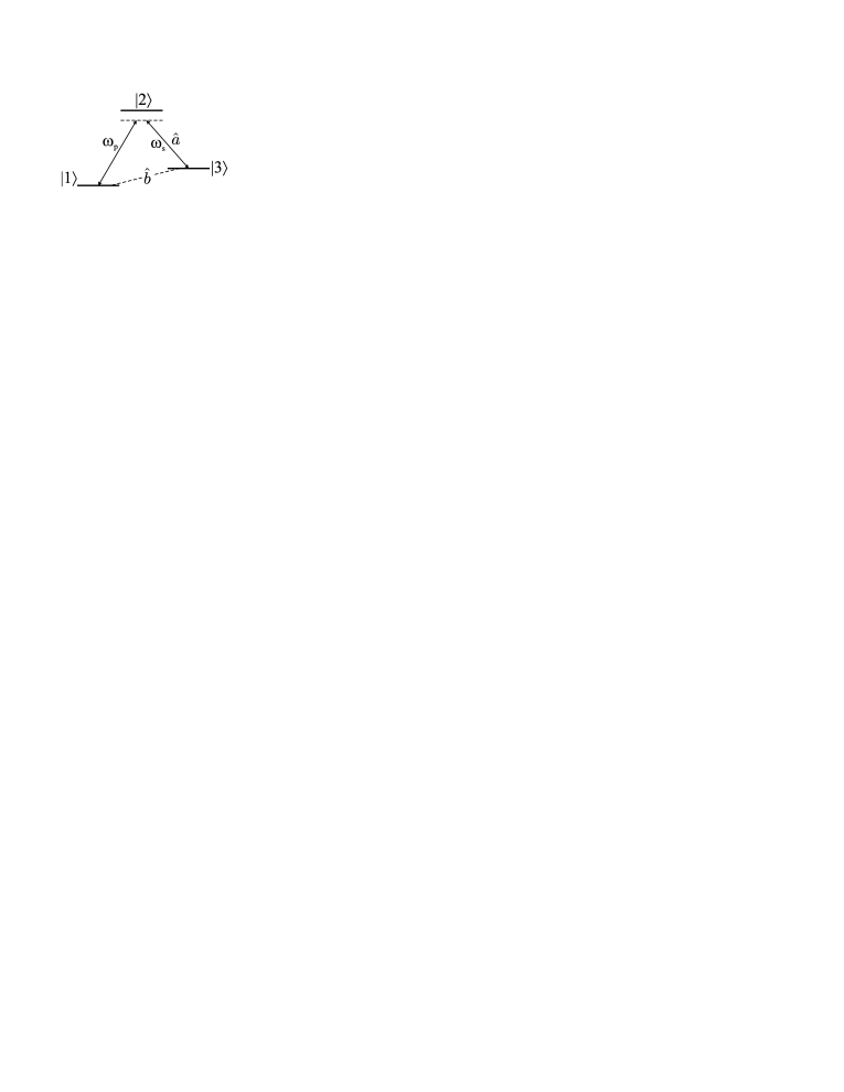
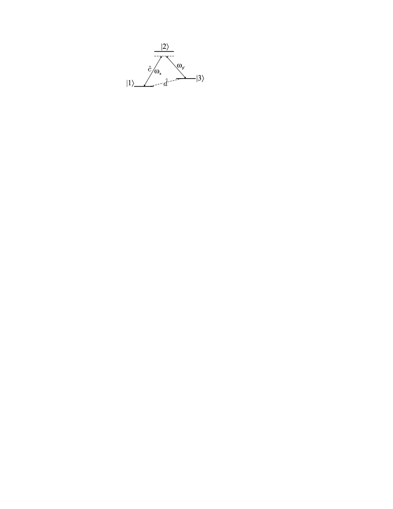
Figure 1: Relevant atomic levels in the Stokes and anti-Stokes (right panel) Raman scattering. Initially atoms reside in state $|1\rangle$. During the first scattering process (left panel) they are driven by strong pump field at a frequency $\omega_{p}$, which creates Stokes optical field $\hat{a}$ at a frequency $\omega_{s}$ and atomic polarization $\hat{b}$. Subsequently, the atoms are subjected to a strong field at a frequency $\omega_{p^{\prime}}$ which erases atomic polarization we will denote by $\hat{d}$ shifting the excitation into anti-Stokes optical field $\hat{c}$ at a frequency $\omega_{a}$ (right panel).

Figure 2: Pictorial representation of the Stokes and subsequent anti-Stokes scattering processes (see Sec. V) in the laboratory reference frame. The vertical stripe represents the cell in which the nonlinear medium is contained, the shaded parallelograms are the spatio-temporal interaction boundaries, the grey (green in color) stripe represents Stokes pump field envelope $A_{p}(z,t)$, while the dark grey (red) stripe represents anti-Stokes pump field envelope $A^{\prime}_{p}(z,t)$. Letters with hats are the annihilation operators of the input and output quantum fields, defined at the respective boundaries of the interaction regions.

II Pair-wise Entanglement Operation

We begin developing our model by idealizing the process of stimulated Raman scattering as a three-wave mixing and restricting ourselves to one dimension Raymer and Mostowski (1981). This is justified provided that atomic saturation and pump field depletion can be neglected while the pump Rayleigh range is comparable to or shorter than the medium length Raymer et al. (1985).

We formulate the equations in the moving reference frame of the Stokes wave

$$t=t_{\text{LAB}}-\frac{z-L/2}{v_{\text{gr,s}}}$$ (1)

where $t_{\text{LAB}}$ is the time in the laboratory frame, $v_{\text{gr,s}}$ is the Stokes group velocity, while $L$ is the medium length. According to the above expression, the laboratory and Stokes reference frames meet in the middle of the medium. Atomic polarization (or spin Lukin (2003)) is described by an operator $\hat{b}(z,t)$ which removes one atom’s worth of internal excitation from the atomic ensemble localized in a thin-slice volume around a point in space-time in the medium Raymer (2004):

$$\hat{b}(z,t)=i\frac{\rho^{1/2}}{n}\sum_{\{\alpha\}_{z}}|1_{\alpha}\rangle\langle 3_{\alpha}|\,e^{i(\omega_{p}-\omega_{s})t_{\text{LAB}}-i(k_{p}-k_{s})z}$$ (2)

where $\rho$ is linear atom density (atoms per mm), $n$ is the number of atoms in a slice, indexed by $\alpha$, $|1\rangle$ and $|3\rangle$ denote the Raman-coupled atomic levels, $\omega_{p}$ and $\omega_{s}$ are the pump and Stokes angular frequencies, while $k_{p}$ and $k_{s}$ are their wavevectors (see Fig. 1). As long as the fraction of excited atoms is small, $\hat{b}(z,t)$ is approximately a bosonic operator, $[\hat{b}(z,t),\hat{b}(z^{\prime},t)^{\dagger}]\approx\delta(z-z^{\prime})$. The Stokes field is described by an envelope annihilation operator at each point in space along the pump beam $\hat{a}(z,t)$:

$$\hat{a}(z,t)=\int d\omega\,e^{-i(\omega-\omega_{s})t_{\text{LAB}}+ik_{s}z}\hat{a}(z,\omega).$$ (3)

It is a bosonic operator, $[\hat{a}(z,t),\hat{a}(z,t^{\prime})^{\dagger}]=\delta(t-t^{\prime})$. Finally, the pump field is given by its envelope $A_{p}(z,t)$ in the reference frame of the Stokes pulse, scaled to unity, defined by

$$\frac{E_{p}(t-(z-L/2)\Delta\beta)}{E_{p,\text{max}}}=A_{p}(z,t)e^{-i\omega_{p}t+ik_{p}z}+\text{c.c.}$$ (4)

where $E_{p}(t)$ is the pump electric field while $\Delta\beta$ is the difference of the inverse group velocities of the pump and Stokes pulses (measured in picoseconds per milimeter)

$$\Delta\beta=\frac{1}{v_{\text{gr,s}}}-\frac{1}{v_{\text{gr,p}}}$$ (5)

where $v_{\text{gr,p}}$ is the pump group velocity. If the Stokes field is faster than the pump, then $\Delta\beta$ is negative.

Using these definitions, the Raman scattering process is cast into the following pair of coupled equations Raymer and Mostowski (1981); Raymer (2004):

$$\frac{\partial\hat{a}(z,t)}{\partial z} = g_{0}A_{p}(z,t)\,\hat{b}^{\dagger}(z,t)$$ (6a)

$$\frac{\partial\hat{b}(z,t)}{\partial t} = g_{0}A_{p}(z,t)\,\hat{a}^{\dagger}(z,t)$$ (6b)

where $g_{0}$ is the coupling constant (measured in $(\text{mm}\text{ps})^{-1/2}$) defined as:

$$g_{0}=\rho^{1/2}\sqrt{\frac{\hbar\omega_{s}}{2\varepsilon_{0}c}}\,E_{p,\text{max}}\kappa_{1}$$ (7)

where $S$ is the pump beam cross-section while $\kappa_{1}$ is a coupling constant defined in Raymer and Mostowski (1981). Since the pump and Stokes pulses are narrowband, higher order dispersion effects, possibly distorting the pulses, can be neglected. On the other hand, in the atomic vapor one finds that the frequency difference between the interacting waves is large enough for significant group velocity differences to be observed. A typical subnanosecond pump pulse can be delayed by several times its duration with respect to the Stokes pulse, thus the presence of nonzero $\Delta\beta$ cannot be neglected Ji et al. .

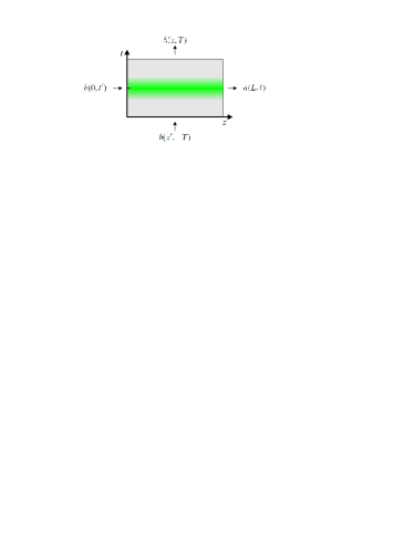
Figure 3: Pictorial representation of the Stokes scattering process in the Stokes reference frame, defined in Eq. (1). The medium entangles light field $\hat{a}$ with atoms $\hat{b}$. The local entanglement amplitude increases with a (fixed) local pump field strength $A_{p}(z,t)$, represented in the picture by a grey (green in color) stripe. Horizontal stripe corresponds to equal group velocities of pump and Stokes, $\Delta\beta=0$.

We proceed with solving Eq. (6) by integrating over a finite spatial-temporal region in which the interaction takes place, thus formulating the problem as a quantum scattering problem. This approach, pictorially represented in Fig. 3 requires introduction of a suitable scattering matrix, which in the case of Stokes scattering is composed of the Green functions of Eq. (6). We choose to introduce them over a space-time region $0<z<L$ and $-T<t<T$, in the following way:

$$\hat{a}(L,t)= \int_{-T}^{T}dt^{\prime}C_{a}(t,t^{\prime})\hat{a}(0,t^{\prime})$$

$$+\int_{0}^{L}dz^{\prime}S_{a}(t,z^{\prime})\hat{b}^{\dagger}(z^{\prime},-T)$$ (8a)

$$\hat{b}(z,T)= \int_{0}^{L}dz^{\prime}C_{b}(z,z^{\prime})\hat{b}(z^{\prime},-T)$$

$$+\int_{-T}^{T}dt^{\prime}S_{b}(z,t^{\prime})\hat{a}^{\dagger}(0,t^{\prime})$$ (8b)

We can simplify the above input-output relations using an extended Bloch-Messiah reduction theorem Braunstein (2005), which we derive in the Appendix A. This theorem states that since the Green functions for this problem must describe a unitary operator transformation, they possess common singular vectors and related singular values $\cosh\zeta_{n}$ and $\sinh\zeta_{n}$:

$$C_{a}(t,t^{\prime})= \sum_{n}\cosh\zeta_{n}\cdot\psi^{(out)*}_{n}(t)\,\psi^{(in)}_{n}(t^{\prime})$$ (9a)

$$C_{b}(z,z^{\prime})= \sum_{n}\cosh\zeta_{n}\cdot\phi^{(out)*}_{n}(z)\,\phi^{(in)}_{n}(z^{\prime})$$ (9b)

$$S_{a}(t,z^{\prime})= \sum_{n}\sinh\zeta_{n}\cdot\psi^{(out)*}_{n}(t)\,\phi^{(in)*}_{n}(z^{\prime})$$ (9c)

$$S_{b}(z,t^{\prime})= \sum_{n}\sinh\zeta_{n}\cdot\phi^{(out)*}_{n}(z)\,\psi^{(in)*}_{n}(t^{\prime}),$$ (9d)

where $\zeta_{n}$ are real numbers while $\psi^{(out)}_{n}(t)$, $\phi^{(out)}_{n}(z)$, $\psi^{(in)}_{n}(t)$ and $\phi^{(in)}_{n}(z)$ are complex-valued functions which form separate orthonormal bases for the output and input, light and atomic mode-function spaces respectively :

$$\int_{-T}^{T}dt\,\psi^{(in)*}_{n}(t)\cdot\psi^{(in)}_{m}(t) =\delta_{n,m}$$ (10)

$$\int_{0}^{L}dz\,\phi^{(in)*}_{n}(z)\cdot\phi^{(in)}_{m}(z) =\delta_{n,m}$$

$$\int_{-T}^{T}dt\,\psi^{(out)*}_{n}(t)\cdot\psi^{(out)}_{m}(t) =\delta_{n,m}$$

$$\int_{0}^{L}dz\,\phi^{(out)*}_{n}(z)\cdot\phi^{(out)}_{m}(z) =\delta_{n,m}.$$

We insert the Green functions in the form given in Eq. (9) into Eq. (8). Then we express input and output field annihilation operators $\hat{a}(0,t)$, $\hat{b}(z,-T)$ by mode expansions and define output operators $\hat{a}(L,t)$ and $\hat{b}(z,T)$ analogously

$$\hat{a}(0,t) =\sum_{n}\hat{a}^{(in)}_{n}\,\psi^{(in)*}_{n}(t)$$ (11)

$$\hat{a}(L,t) =\sum_{n}\hat{a}^{(out)}_{n}\,\psi^{(out)*}_{n}(t)$$

$$\hat{b}(z,-T) =\sum_{n}\hat{b}^{(in)}_{n}\,\phi^{(in)*}_{n}(z)$$

$$\hat{b}(z,T) =\sum_{n}\hat{b}^{(out)}_{n}\,\phi^{(out)*}_{n}(z),$$

where we have introduced operators $\hat{a}^{(in)}_{n}$, $\hat{a}^{(out)}_{n}$, $\hat{b}^{(in)}_{n}$ and $\hat{b}^{(out)}_{n}$. Thanks to orthonormality of the respective mode functions expressed in Eq. (10), these operators obey canonical commutational relations:

$$[\hat{a}^{(out)}_{n},\hat{a}^{(out)\dagger}_{m}] =\delta_{nm} [\hat{b}^{(out)}_{n},\hat{b}^{(out)\dagger}_{m}] =\delta_{nm}$$ (12)

and the operators with superscript $(in)$ obey analogous commutational relations. Therefore $\hat{a}^{(in)}_{n}$, $\hat{a}^{(out)}_{n}$, $\hat{b}^{(in)}_{n}$ and $\hat{b}^{(out)}_{n}$ are bosonic operators, which annihilate excitations in respective light and atomic modes. Using Eq. (9), (10) and (11), Eq. (8) can be cast into the following form:

$$\hat{a}^{(out)}_{n} = \hat{a}^{(in)}_{n}\cosh\zeta_{n}+\hat{b}^{(in)\dagger}_{n}\sinh\zeta_{n}$$ (13a)

$$\hat{b}^{(out)}_{n} = \hat{b}^{(in)}_{n}\cosh\zeta_{n}+\hat{a}^{(in)\dagger}_{n}\sinh\zeta_{n}.$$ (13b)

This expresses independent two-mode squeezing processes, and is the main result of this part of our study. Each of these elementary processes squeezes the optical field in a particular temporal mode $\psi^{(in)}_{n}(t)$ with the atomic polarization in a particular longitudinal spatial mode $\phi^{(in)}_{n}(z)$, producing fields in optical temporal modes $\psi^{(out)}_{n}(t)$ that are pair-wise entangled with the internal states of atoms described by collective spatial modes $\phi^{(out)}_{n}(z)$. The squeezing parameter equals $\zeta_{n}$. The noise in the sum and difference of quadratures scales by a factor of $\exp(\zeta_{n})$, corresponding to the mean number of excitations $\langle\hat{n}_{n}\rangle=\langle\hat{a}^{(out)\dagger}_{n}\hat{a}^{(out)}_{n}\rangle=\langle\hat{b}^{(out)\dagger}_{n}\hat{b}^{(out)}_{n}\rangle=\sinh^{2}\zeta_{n}$.

Note that for a pump pulse of a given shape, characterized by duration $\tau_{p}$, for instance Gaussian:

$$A_{p}(z,t)=\exp\left[-2\ln 2\,\left(\frac{t-(z-L/2)\Delta\beta}{\tau_{p}}\right)^{2}\right],$$ (14)

the time and space in equations (6) can be reduced to a dimensionless coordinates by measuring time in units of pump pulse duration $\tau_{p}$ and space in units of distance over which temporal Stokes walk-off equals pump duration $\tau_{p}/\Delta\beta$. This way the pump envelope $A_{p}(\Delta\beta z/\tau_{p},t/\tau_{p})$ becomes a fixed function. Note that for $T\gg\tau_{p}$ the Green functions do not depend on $T$ since there is no longer any interaction taking place for large $t$. Thus the Green functions defined in Eq. (8) can depend only on medium length, coupling strength, and pulse shape. Both can be brought into a form of two dimensionless parameters:

$$\Delta =\frac{L\Delta\beta}{\tau_{p}}$$ (15a)

$$\Gamma =g_{0}\sqrt{L\tau_{p}}\,.$$ (15b)

The first is the temporal walkoff between pump and Stokes field, measured in pump pulse durations, while the second measures the squeezing strength and is proportional to the squeezing parameter in the case of zero dispersion Raymer and Mostowski (1981); Raymer (2004). Therefore there is a congruence between the solutions and mode functions for the Stokes scattering problem, as long as the pump pulse shapes are congruent and the values of the parameters $\Gamma$ and $\Delta$ are the same.

Finally, let us note that the characteristic output modes $\psi^{(out)}_{n}(t)$ and $\phi^{(out)}_{n}(t)$ we obtained with the help of the Bloch-Messiah reduction are identical to previously obtained atomic and field coherence modes Raymer et al. (1985); Raymer (2004); Raymer et al. (1989). The latter were introduced as the eigenmodes of the first-order coherence functions for atoms $\langle\hat{b}(z,T)\hat{b}^{\dagger}(z^{\prime},T)\rangle$ and field $\langle\hat{a}(L,t)\hat{a}^{\dagger}(L,t^{\prime})\rangle$. Calculating these functions explicitly using equations (9) we obtain:

$$\langle\hat{a}(L,t)\hat{a}^{\dagger}(L,t^{\prime})\rangle= \int_{0}^{L}dz^{\prime}S_{a}(t,z^{\prime})S^{*}_{a}(t^{\prime},z^{\prime})$$

$$= \sum_{n}\langle\hat{n}_{n}\rangle\,\psi^{(out)*}_{n}(t)\,\psi^{(out)}_{n}(t^{\prime})$$ (16)

$$\langle\hat{b}(z,T)\hat{b}^{\dagger}(z^{\prime},T)\rangle= \int_{-T}^{T}dt^{\prime}S_{b}(z,t^{\prime})S^{*}_{b}(z^{\prime},t^{\prime})$$

$$= \sum_{n}\langle\hat{n}_{n}\rangle\,\phi^{(out)*}_{n}(t)\,\phi^{(out)}_{n}(t^{\prime})$$ (17)

as in Raymer et al. (1985); Raymer (2004). In Raymer (2004) also the characteristic input modes were introduced as those evolving into a particular pair of output modes, which is another way of obtaining the decomposition given in Eq. (9).

III Numerical Results

To illustrate the meaning of the above results and provide the decomposition into independent entanglement processes in some specific and realistic cases, we have numerically found Green functions defined in Eq. (8). Calculations were carried out for a medium of length $L=75\,$mm for various values of group velocity difference $\Delta\beta$, coupling strength $g_{0}$ and Gaussian pump pulse of FWHM duration $\tau_{p}=200\,$ps as defined in Eq. (14).

As the equations of motion (6) are linear, they are identical to the classical equations for evolution of the Stokes field and the atomic polarization in the case of stimulated Raman scattering, in which annihilation operators $\hat{a}(z,t)$ and $\hat{b}(z,t)$ are replaced by classical field $\alpha(z,t)$ and polarization amplitudes $\beta(z,t)$. Therefore we can compute matrix approximations to the Green functions $C_{a}(t,t^{\prime})$, $C_{b}(z,z^{\prime})$, $S_{a}(t,z^{\prime})$ and $S_{b}(z,t^{\prime})$ using standard methods developed in nonlinear optics. To accomplish this, equations (6) were solved numerically for a complete orthonormal set of initial conditions. First we put $\alpha(0,t)=0$ for every $t$ except for a single point on a computational grid $t=t^{\prime}$ where $\alpha(0,t^{\prime})=1$, and $\beta(z,-T)=0$ for every $z$. Performing finite integration steps over the space-time grid of 200$\times$200 points where the interaction occurs, we computed $\alpha(L,t)$ and $\beta(z,T)$. For the initial conditions chosen, they are equal to $C_{a}(t,t^{\prime})$ and $S_{b}(z,t^{\prime})$, respectively. Repeating this calculation for each $t^{\prime}$, we constructed a matrix approximation of these Green functions. Then analogously starting from $\alpha(0,t)=0$, and $\beta(z,-T)=0$ except for a single point on a computational grid where $\beta(z^{\prime},-T)=1$, we have constructed $C_{b}(z,z^{\prime})$, $S_{a}(t,z^{\prime})$. Next we numerically performed the singular value decomposition Golub and Loan (1996) of these matrices to obtain the singular values $\sinh\zeta_{n}$ and $\cosh\zeta_{n}$ as well as associated vectors $\psi^{(in)}_{n}(t)$, $\phi^{(in)}_{n}(t)$, $\psi^{(out)}_{n}(t)$ and $\phi^{(out)}_{n}(t)$ as defined in Eq. (9). We have verified that our simulation is accurate by repeating it on a grid two times finer in each dimension. The differences between the results were of the order of precision with which singular value decomposition can be computed. We have also verified that our numerical calculation reconstructs the analytical results for square pump pulse without dispersion Raymer (2004).

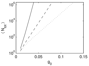
Figure 4: Mean number of Stokes photons as a function of coupling strength $g_{0}$ [(mm ps)^-1/2]. Three lines are the results of computations for different $\Delta\beta$ equal $0$ (solid line), $-10\,$ps/mm (dashed line) and $-30\,$ps/mm (dotted line).

Numerical calculations confirm that the total number of photons

$$\langle N_{\text{tot}}\rangle=\sum_{n}\langle\hat{n}_{n}\rangle=\sum_{n}\sinh^{2}\zeta_{n}.$$ (18)

is, to a good approximation, an exponential function of coupling $g_{0}$, within the range plotted in Fig. 4. However, we find a strong dependence of $\langle N_{\text{tot}}\rangle$ on the group velocity difference between pump and Stokes pulses $\Delta\beta$. With increasing $\Delta\beta$ the total photon number $\langle N_{\text{tot}}\rangle$ quickly decreases. Using results displayed in Fig. 4 we have found, for each $\Delta\beta$, the value of coupling $g_{0}$ for which the total number of photons equals $\langle N_{\text{tot}}\rangle=10^{6}$. These values of coupling $g_{0}$ will be used in the following examples.

$\langle\hat{n}_{n}\rangle$

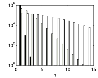
Figure 5: Mean number of photons in each of characteristic output modes $\langle\hat{n}_{n}\rangle$ for 15 most-occupied modes. The histograms has been made for coupling yielding average total number of Stokes photons $\langle N_{\text{tot}}\rangle=10^{6}$ for different $\Delta\beta$ equal $0$ (black bar), $-10\,$ps/mm (grey bars) and $-30\,$ps/mm (empty bars).

In Fig. 5 we plot the mean number of photons in each mode $\langle\hat{n}_{n}\rangle=\sinh^{2}\zeta_{n}$. In the case of no dispersion $\Delta\beta=0$, the occupation of the first mode dominates by a factor of $10^{3}$ over the next, as known previously Raymer et al. (1982); Walmsley and Raymer (1983). Strong domination, however, quickly comes to an end with increasing dispersion. For $\Delta\beta=-30\,$ps/mm more than a dozen modes have occupancy equal within an order of magnitude.

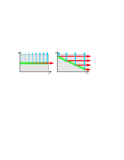
Figure 6: Pictorial representation of the Stokes scattering for zero group velocity difference $\Delta\beta$ (left) and large negative $\Delta\beta\ll-\tau_{p}/L$ (right). The grey box represents the spatio-temporal region of interaction, the dark grey (green in color) stripe is the pumped region, the horizontal (red) arrows are the Stokes emission, while the vertical (blue) arrows represent atomic polarization. The picture has been drawn in the Stokes reference frame.

$\Delta\beta=0$	$\Delta\beta=-10\,$ps/mm	$\Delta\beta=-30\,$ps/mm

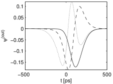
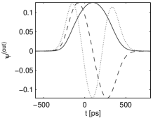
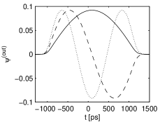
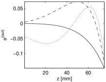
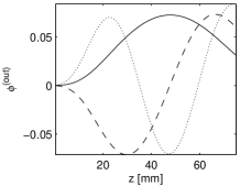
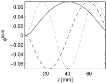
Figure 7: Optical $\psi^{(out)}_{n}(t)$ and atomic $\phi^{(out)}_{n}(t)$ output mode functions for three most excited modes, $n=1$ (solid line), $n=2$ (dashed line) and $n=3$ (dotted line) for various group velocity differences $\Delta\beta$.

The physical reason behind this result can be traced in Fig. 6, where we depict a space-time region where the interaction occurs. We mark the pumped area as the dark grey (green) region. In the case of zero group velocity difference, $\Delta\beta=0$, the first few Stokes photons propagate through the pumped region, stimulating subsequent scattering acts and inducing coherence between atomic polarization in various regions along the cell. The process is almost single mode Raymer et al. (1982); Raymer (2004). On the other hand, in the case of high group velocity difference, the spatial-temporal interaction region can be divided into several regions, the number of such regions being roughly the ratio of the total temporal walkoff to the pump duration $\Delta=L\Delta\beta/\tau_{p}$. These regions are weakly coupled, since the photons scattered in the distinct parts of the cell do not have a chance to meet each other. Thus several uncorrelated temporal modes take part in the process and become significantly occupied.

This latter phenomenon complicates the possible applications. For nonzero dispersion one must afford means, such as for example balanced homodyne detection, for separating distinct output modes in order to extract a pure squeezed state of light and matter. Whether in the single or multimode squeezing regime, an efficient detection of Stokes light is necessary for quantum communication and computation. This is possible by means of balanced homodyne detection using a local oscillator in the shape of the characteristic Stokes mode. In Fig. 7 we plot the temporal shape of the most occupied output field modes for the Gaussian pump centered at $t=0$ defined in (14). The dominant mode has a single peak, which is time delayed relative to pump peak Raymer et al. (1989). The modes resemble in shape the eigenmodes of a harmonic oscillator. They are also strongly affected by the group velocity difference. With increasing $\Delta\beta$, the duration of the fundamental mode increases while the time delay relative to the pump pulse in the middle of the medium decreases. Also for large $\Delta\beta$ all the characteristic modes have significant intensity over the same period of time, spanning approximately one pump duration plus temporal walkoff between pump and the Stokes $\tau_{p}+L\Delta\beta=\tau_{p}(1+\Delta)$.

Note that in the limit of zero dispersion, $\Delta\beta=0$, the Green functions calculated numerically can be found in a closed form using Laplace-transform techniques Raymer and Mostowski (1981), even for the full three-dimensional case Raymer et al. (1985). The results presented here for zero dispersion are recovered by applying numerical diagonalization directly to those functions Raymer (2004). Finally let us note that the output characteristic modes can be used to reconstruct the statistics of fluctuating Stokes pulse shapes Raymer et al. (1989).

IV Photon count statistics

Using the results of numerical calculations, we were able to compute the photon-count statistics for the Stokes pulse. Let us recall that one mode of the pair comprising a two-mode squeezed state exhibits thermal statistics. This is the case of any particular output field mode $\psi^{(out)}_{n}(t)$ by itself. Also, each of the output field modes is independent, since they evolve separately from vacuum. Thus the Stokes pulse has multimode thermal statistics Raymer et al. (1982):

$$p(n)=\frac{1}{2\pi}\int dk\frac{e^{-ikn}}{\prod_{n}(1-ik\langle\hat{n}_{n}\rangle)}$$ (19)

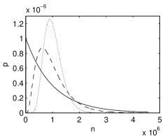
Figure 8: Photon count probability distribution $p(n)$ of Stokes light pulses. Three lines are the results of computations for different $\Delta\beta$ equal $0$ (solid line), $-10\,$ps/mm (dashed line) and $-30\,$ps/mm (dotted line).

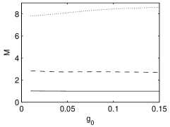
Figure 9: Equivalent number of independent thermal modes $\mathcal{M}$ as a function of coupling strength $g_{0}$ [(mm ps)^-1/2]. Three lines are the results of computations for different $\Delta\beta$ equal $0$ (solid line), $-10\,$ps/mm (dashed line) and $-30\,$ps/mm (dotted line).

We plot $p(n)$ in Fig. 8 for total photon number $\langle N_{\text{tot}}\rangle=10^{6}$ and various values of group velocity difference $\Delta\beta$.

Following the analogy with thermal light, we have also computed and plot in Fig. 9 the equivalent number of modes $\mathcal{M}$. It is defined as a number of independent thermal modes of equal intensity that measured together reproduce the Stokes fluctuation-to-mean ratio:

$$\mathcal{M}=\frac{\langle N_{tot}\rangle^{2}}{\sum_{n}\langle\hat{n}_{n}\rangle^{2}.}$$ (20)

As can be seen in Fig. 9, the equivalent mode number $\mathcal{M}$ depends mostly on $\Delta\beta$, which is almost independent of coupling strength $g_{0}$. This is consistent with the intuitive way of understanding Stokes scattering we propose in Fig. 6.

V Atomic polarization readout

As shown in Section II, the optical Stokes pulse contains only one part of the squeezed state. Alone it has thermal statistics and possesses no distinct quantum features. Entanglement can be observed only if the field counterpart — the atomic polarization — is acted upon. A convenient to way process the atomic $\hat{b}(z)$ field is to translate its statistics into the optical field. This is done in the anti-Stokes scattering process, during which a portion of atomic polarization gives rise to an anti-Stokes pulse. The equations governing this process are similar to Eqs. (6) in the anti-Stokes reference frame Raymer (2004):

$$\frac{\partial\hat{c}(z,t)}{\partial z} = g^{\prime}_{0}A^{\prime}_{p}(z,t)\hat{d}(z,t)$$ (21a)

$$\frac{\partial\hat{d}(z,t)}{\partial t} = -g^{\prime*}_{0}A^{\prime*}_{p}(z,t)\hat{c}(z,t)$$ (21b)

where $\hat{c}(z,t)$ is the anti-Stokes field annihilation operator, defined by an equation analogous to (3), $\hat{d}(z,t)$ is the atomic polarization operator, defined by an equation analogous to (2), $g^{\prime}_{0}$ is the readout coupling defined analogously to (7), while $A^{\prime}_{p}(z,t)$ is the readout pump field envelope. The definition of the $A^{\prime}_{p}(z,t)$ is analogous to that of the Stokes pump field envelope $A_{p}(z,t)$ given in Eq. (4), but with a different peak amplitude and a different group velocity difference, which we will designate by $\Delta\beta^{\prime}$:

$$\Delta\beta^{\prime}=\frac{1}{v_{\text{gr,a}}}-\frac{1}{v_{\text{gr,p}}}$$ (22)

where $v_{\text{gr,a}}$ is the group velocity of the anti-Stokes wave, while $v_{\text{gr,p}}$ is the group velocity of the readout pump.

Again, we formulate the readout problem as a quantum scattering problem, analogously to the situation illustrated in Fig. 3. This time the scattering matrix is composed of four Green functions for the anti-Stokes scattering equations (21). We define them analogously to those defined in Eq. (8) for the Stokes scattering:

$$\hat{c}(L,t) = \int_{-T}^{T}dt^{\prime}C_{c}(t,t^{\prime})\hat{c}(0,t^{\prime})$$ (23a)

$$+\int_{0}^{L}dz^{\prime}S_{c}(t,z^{\prime})\hat{d}(z^{\prime},-T)$$

$$\hat{d}(z,T) = \int_{0}^{L}dz^{\prime}C_{d}(z,z^{\prime})\hat{d}(z^{\prime},-T)$$ (23b)

$$-\int_{-T}^{T}dt^{\prime}S_{d}(z,t^{\prime})\hat{c}(0,t^{\prime})$$

Here $\hat{c}(0,t)$ is the optical field operator (usually representing the vacuum) entering the vapor during readout, and $\hat{d}(z,-T)$ is the atomic ensemble operator just prior to the readout.

We can cast these relations into multiple, independent beamsplitter transformations (see Appendix B). Since the Green functions for this problem must describe a unitary transformation, they possess common singular vectors and related singular values, which we parameterize by $\eta_{n}$:

$$C_{c}(t,t^{\prime})= \sum_{n}\sqrt{1-\eta_{n}}\cdot\Psi^{(out)*}_{n}(t)\,\Psi^{(in)}_{n}(t^{\prime})$$ (24a)

$$C_{d}(z,z^{\prime})= \sum_{n}\sqrt{1-\eta_{n}}\cdot\Phi^{(out)*}_{n}(z)\,\Phi^{(in)}_{n}(z^{\prime})$$ (24b)

$$S_{c}(t,z^{\prime})= \sum_{n}\sqrt{\eta_{n}}\cdot\Psi^{(out)*}_{n}(t)\,\Phi^{(in)}_{n}(z^{\prime})$$ (24c)

$$S_{d}(z,t^{\prime})= \sum_{n}\sqrt{\eta_{n}}\cdot\Phi^{(out)*}_{n}(z)\,\Psi^{(in)}_{n}(t^{\prime}).$$ (24d)

The readout modes $\Psi^{(out)}_{n}(t)$, $\Phi^{(out)}_{n}(z)$, $\Psi^{(in)}_{n}(t)$ and $\Phi^{(in)}_{n}(z)$ form orthonormal bases in the intput/output, light and atomic modefunction spaces:

$$\int_{-T}^{T}dt\,\Psi^{(in)*}_{n}(t)\cdot\Psi^{(in)}_{m}(t) =\delta_{n,m}$$ (25)

$$\int_{0}^{L}dz\,\Phi^{(in)*}_{n}(z)\cdot\Phi^{(in)}_{m}(z) =\delta_{n,m}$$

$$\int_{-T}^{T}dt\,\Psi^{(out)*}_{n}(t)\cdot\Psi^{(out)}_{m}(t) =\delta_{n,m}$$

$$\int_{0}^{L}dz\,\Phi^{(out)*}_{n}(z)\cdot\Phi^{(out)}_{m}(z) =\delta_{n,m}.$$

We use these functions as mode bases in respective spaces and decompose the annihilation operators $\hat{c}(0,t)$, $\hat{c}(L,t)$, $\hat{d}(z,-T)$ and $\hat{d}(z,T)$:

$$\hat{c}(0,t) =\sum_{n}\hat{c}^{(in)}_{n}\,\Psi^{(in)*}_{n}(t)$$ (26a)

$$\hat{c}(L,t) =\sum_{n}\hat{c}^{(out)}_{n}\,\Psi^{(out)*}_{n}(t)$$ (26b)

$$\hat{d}(z,-T) =\sum_{n}\hat{d}^{(in)}_{n}\,\Phi^{(in)*}_{n}(z)$$ (26c)

$$\hat{d}(z,T) =\sum_{n}\hat{d}^{(out)}_{n}\,\Phi^{(out)*}_{n}(z).$$ (26d)

Where we have introduced annihilation operators of the input and output characteristic modes $\hat{c}^{(in)}_{n}$, $\hat{d}^{(in)}_{n}$, $\hat{c}^{(out)}_{n}$ and $\hat{d}^{(out)}_{n}$. Again, it turns out that the output operators $\hat{c}^{(out)}_{n}$ and $\hat{d}^{(out)}_{n}$ are independent bosonic operators. Same is true for input operators $\hat{c}^{(in)}_{n}$ and $\hat{d}^{(in)}_{n}$.

These operators annihilate excitations of modes that undergo transformations analogous to a beamsplitter transformation:

$$\hat{c}^{(out)}_{n} = \sqrt{1-\eta_{n}}\,\hat{c}^{(in)}_{n}+\sqrt{\eta_{n}}\,\hat{d}^{(in)}_{n}$$ (27a)

$$\hat{d}^{(out)}_{n} = \sqrt{1-\eta_{n}}\,\hat{d}^{(in)}_{n}-\sqrt{\eta_{n}}\,\hat{c}^{(in)}_{n}.$$ (27b)

The real parameters $\eta_{n}$ have the meaning of the readout efficiency. Modes with $\eta_{n}=1$ are completely translated from the atomic field into the optical field while spatial modes with $\eta_{n}=0$ remain unaffected by the anti-Stokes scattering process.

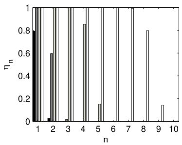
Figure 10: Readout efficiency $\eta_{n}$ for the most efficiently read modes in anti-Stokes scattering process for $\Delta\beta^{\prime}=0$ and coupling $g^{\prime}_{0}$ equal $0.01,\,0.02,\,0.05,\,0.1\,(\text{ps}\,\text{mm})^{-1/2}$, for black, grey and empty bars respectively.

We have numerically found forms for the Green functions defined in Eq. (23) for similar conditions used to calculate the Raman process in earlier sections. Results are first presented for the case of a medium of length $L=75\,$mm with zero group velocity difference $\Delta\beta^{\prime}$, various coupling strengths $g^{\prime}_{0}$ and Gaussian pump pulse $A^{\prime}_{p}(z,t)$ of FWHM duration $\tau^{\prime}_{p}=200\,$ps given in Eq. (14). In Fig. 10 we plot the calculated $\eta_{n}$. It can be seen that above a certain value of coupling $g^{\prime}_{0}$, many modes have unit readout efficiency $\eta_{n}=1$, i.e. are completely translated into the optical field. Those modes are degenerate, thus within a subspace spanned by their mode functions we can change the basis, i.e. the modal functions, without affecting relations (27).

Let us focus on the case that the readout takes place just following the Raman scattering process described in earlier sections; in this case $\hat{d}(z,-T)$ is given by the output operator $\hat{b}(z,T)$ in Eq. (8):

$$\hat{d}(z,-T)=e^{i\Delta k\,z}\,\hat{b}(z,T)$$ (28)

where $\Delta k$ is the wavevector mismatch in the time-delayed four-wave mixing process:

$$\Delta k=k_{p}-k_{s}+k_{a}-k_{p^{\prime}}\,,$$ (29)

where subscript $p$, $p^{\prime}$, $s$, $a$ denote Stokes pump and anti-Stokes pump, Stokes and anti-Stokes signal waves respectively. For efficient readout the phase-matching condition $\Delta k=0$ must be satisfied. Below we will assume perfect phasematching. It is possible to satisfy this by proper choice of pump frequencies.

Using the expansions (11) and (26) we find that the characteristic anti-Stokes input operators $\hat{d}^{(in)}_{n}$ are related to the characteristic Stokes output operators $\hat{b}^{(out)}_{n}$ by an unitary transformation expressing the change of basis from $\phi^{(out)}_{n}(z)$ to $\Phi^{(in)}_{n}(z)$:

$$\hat{d}^{(in)}_{m}=\sum_{n}\mathbf{U}_{mn}\hat{b}^{(out)}_{n}$$ (30)

where the transformation coefficients are:

$$\mathbf{U}_{mn}=\int_{0}^{L}dz\,\phi^{(out)*}_{n}(z)e^{-i\Delta kz}\cdot\Phi^{(in)}_{m}(z).$$ (31)

Let us consider the readout of the first characteristic atomic mode of the Stokes scattering $\phi^{(out)}_{1}(z)$ whose quantum statistics, before the readout, is contained in the operator $\hat{b}^{(out)}_{1}$. It can be decomposed in the characteristic anti-Stokes input mode base $\Phi^{(in)}_{n}(z)$, according to the above formulas. The readout has unit efficiency if the atomic mode $\phi^{(out)}_{1}(z)$ decomposes only into readout characteristic input modes $\Phi^{(in)}_{n}(z)$ for which $\eta_{m}=1$. In other words, if for all $m$ for which $\mathbf{U}_{m1}\neq 0$ the readout efficiencies $\eta_{m}$ equal one, then the readout has unit efficiency.

There is however a more straightforward way to analyze a readout of an excitation in a particular mode. Assuming perfect phase matching, $\Delta k=0$, so $\hat{d}(z,-T)=\hat{b}(z,T)$ we substitute input atomic operator $\hat{d}(z,-T)$ in Eq. (23) by $\hat{b}(z,T)$ in an expanded form given by Eq. (11):

$$\hat{c}(L,t) =\sum_{n}\sigma^{*}_{n}(t)\hat{b}^{(out)}_{n}+\int_{-T}^{T}dt^{\prime}C_{c}(t,t^{\prime})\hat{c}(0,t^{\prime})$$ (32a)

$$\hat{d}(z,T) =\sum_{n}\varepsilon^{*}_{n}(z)\hat{b}^{(out)}_{n}-\int_{-T}^{T}dt^{\prime}S_{d}(z,t^{\prime})\hat{c}(0,t^{\prime})$$ (32b)

where we have introduced mode functions

$$\sigma^{*}_{n}(t)= \int_{0}^{L}dz^{\prime}\,S_{c}(t,z^{\prime})\,\phi^{(out)*}_{n}(z^{\prime})$$ (33a)

$$\varepsilon^{*}_{n}(z)= \int_{0}^{L}dz^{\prime}\,C_{d}(z,z^{\prime})\,\phi^{(out)*}_{n}(z^{\prime}).$$ (33b)

The equations (32) give yet another modal decomposition of the output atomic and light fields. However this time the modal functions: $\sigma^{*}_{n}(t)$, $C_{c}(t,t^{\prime})$, $\varepsilon^{*}_{n}(z)$ and $S_{d}(z,t^{\prime})$ form othonormal bases in the joint atom-light space:

$$\int_{-T}^{T}dt\,\sigma^{*}_{n}(t)\sigma_{m}(t)+\int_{0}^{L}dz\,\varepsilon^{*}_{n}(z)\varepsilon_{m}(z)=\delta_{mn}$$ (34a)

$$\int_{-T}^{T}dt\,\sigma^{*}_{n}(t)C_{c}(t,t^{\prime})-\int_{0}^{L}dz\,\varepsilon^{*}_{n}(z)S_{d}(z,t^{\prime})=0.$$ (34b)

This is a consequence of unitarity of the relations (23) (see also Appendix B).

Usually we want statistics of some particular atomic mode, say $\phi^{(out)}_{1}(z)$, to be completely transferred into an optical field mode. This requirement is equivalent to requesting $\varepsilon_{1}(z)=0$ for every $z$, so that $\hat{d}(z,T)$ in Eq. (32b) contains only zero-point, vaccum noise represented by $\hat{c}(0,t^{\prime})$. The output light mode $\sigma_{1}(t)$ can be computed in advance and detection apparatus tuned to it. Note, that if the transfer is complete the $z$ integrals containing $\varepsilon_{1}(z)$ vanish in Eq. (34). It follows that all other output field modes must be orthogonal to $\sigma_{1}(t)$. In other words no crosstalk occurs, i.e. the polarization in any other atomic mode does not give rise to any photons in the optical field mode $\sigma_{1}(t)$ we are presumably tuned to. This does not prevent emission into other optical modes, however.

Therefore the readout problem can be reduced to a question of how to prepare the readout pump pulse in such a way that the atomic polarization of interest, say in mode $\phi^{(out)}_{1}(z)$, is completely transferred into the optical field.

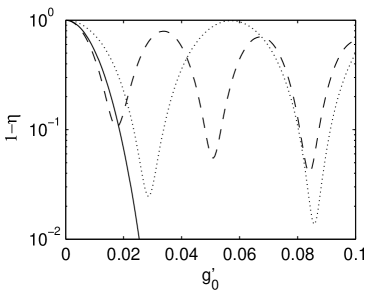
Figure 11: Fraction of residual atomic polarization $1-\eta$ not transferred to an optical field after the anti-Stokes scattering process as a function of the readout coupling $g_{0}\,[(\text{ps}\,\text{mm})^{-1/2}]$. Results for three group velocity differences $\Delta\beta^{\prime}$ equal $0$ (solid line), $-10\,$ps/mm (dashed line) and $-30\,$ps/mm (dotted line) are displayed.

	$\Delta\beta^{\prime}=0$	$\Delta\beta^{\prime}=-10\,$ps/mm	$\Delta\beta^{\prime}=-30\,$ps/mm
$\sigma_{1}(t)$
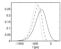
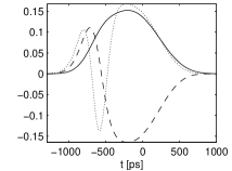
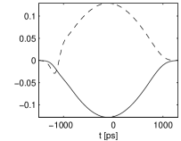
	$g^{\prime}_{0}=0.04,0.07,0.1$	$g^{\prime}_{0}=0.018,0.05,0.084$	$g^{\prime}_{0}=0.028,0.086$ (mm ps)-1/2

Figure 12: Readout anti-Stokes light modes $\sigma_{1}(t)$ for fundamental atomic Stokes modes $\phi^{(out)}_{1}(z)$ for various group velocity difference $\Delta\beta=\Delta\beta^{\prime}$ and coupling strengths corresponding to readout efficiency peaks for nonzero $\Delta\beta^{\prime}$ (compare Fig. 11). Solid, dashed and dotted lines correspond respectively to subsequent values of $g^{\prime}_{0}$, listed below each panel.

We investigated this by simulating readout of an atomic mode $\phi^{(out)}_{1}(z)$ in an anti-Stokes interaction. Calculations were carried out for a medium of length $L=75\,$mm for various values of group velocity differences, assuming $\Delta\beta=\Delta\beta^{\prime}$. For each particular value of this parameter, we have first computed the mode function of the fundamental atomic output mode $\phi^{(out)}_{1}(z)$ in a way described in Sec. III, with the Stokes coupling such that the total mean number of excitations $\langle N_{\text{tot}}\rangle=10^{6}$. Next we have simulated the anti-Stokes scattering of this particular atomic mode for various anti-Stokes coupling strengths $g^{\prime}_{0}$ and Gaussian pump $A^{\prime}_{p}(z,t)$ of FWHM duration $\tau^{\prime}_{p}=200\,$ps given in Eq. (14). We have quantified the quality of the readout by computing the residual fraction of atomic polarization after the readout

$$1-\eta=\int_{0}^{L}dz|\varepsilon_{1}(z)|^{2}$$ (35)

The results are shown in Fig. 11. One can see that for zero group velocity difference $1-\eta$ rapidly falls with increasing coupling $g^{\prime}_{0}$ as predicted in Raymer (2004). The readout is virtually perfect for $g^{\prime}_{0}>0.04\,(\text{ps}\,\text{mm})^{-(1/2)}$. However for nonzero $\Delta\beta^{\prime}$ the residual atomic polarization is of the order of at least a percent. The readout inefficiency $1-\eta$ becomes a periodic function of coupling $g^{\prime}_{0}$. The period increases with increasing $\Delta\beta^{\prime}$, and the particular optimal values of $g^{\prime}_{0}$ depend on the parameters of the readout process as well as the initial atomic excitation mode function $\phi^{(out)}_{1}(z)$.

In Fig. 12 we plot the output field modes $\sigma_{1}(t)$ obtained in the readout simulations. In case of homodyne detection of the output of the anti-Stokes readout process, those would be the optimal local oscillator shapes. For zero group velocity difference $\Delta\beta^{\prime}=0$ we observe that the output field mode becomes shorter with increasing $g^{\prime}_{0}$. For nonzero $\Delta\beta^{\prime}$ the mode shapes $\sigma_{1}(t)$ corresponding to the subsequent minima of the function $1-\eta(g^{\prime}_{0})$ depicted in the Fig. 11 show increasing number of nodes.

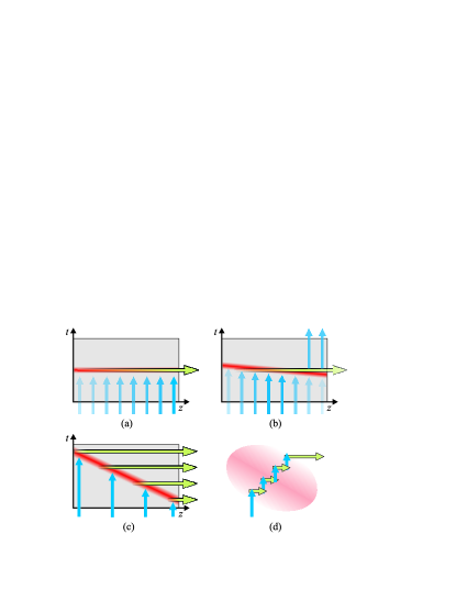
Figure 13: Pictorial representation of the anti-Stokes scattering for zero group velocity difference $\Delta\beta^{\prime}$ (a), medium value of $\Delta\beta^{\prime}$ (b) and high negative $\Delta\beta^{\prime}\ll-\tau_{p}/L$ (c). The grey box represents the spatio-temporal region of interaction, the dark grey (red in color) stripe is the pumped region, the horizontal (green) arrows are the anti-Stokes emission, while the vertical (blue) arrows represent atomic polarization. The picture is drawn in the anti-Stokes reference frame. Panel (d) gives insight into oscillatory exchange of excitation between light and atoms.

The physics behind the readout process can be intuitively understood if one notes that integrating the propagation equations (21) over a spatiotemporal region $2\Delta z\times 2\Delta t$ where the fields are almost constant gives a simple beamsplitter-like relation between input and output fields:

$$\hat{c}(z+\Delta z,t)= \hat{c}(z-\Delta z,t)\sqrt{1-|\gamma|^{2}}+\gamma\hat{d}(z,t-\Delta t)\frac{\sqrt{\Delta z}}{\sqrt{\Delta t}}$$

$$\hat{d}(z,t+\Delta t)= \hat{d}(z,t-\Delta t)\sqrt{1-|\gamma|^{2}}-\gamma^{*}\hat{c}(z-\Delta z,t)\frac{\sqrt{\Delta t}}{\sqrt{\Delta z}}$$ (36)

where $\gamma=2g^{\prime}_{0}A^{\prime}_{p}(z,t)\sqrt{\Delta z\Delta t}$. Therefore we can visualize the scattering process as a square network of virtual beamsplitters, each having different reflectivity $\sqrt{\gamma}$. In Fig. 13 we represent the pumping intensity $A^{\prime}_{p}(z,t)$ and the beams representing atomic polarization and optical field, which propagate in above mentioned network.

For zero group velocity difference and a nearly exponential input atomic mode $\phi^{(out)}_{1}(z)$ (see Fig. 7a) the anti-Stokes field grows with $z$ sweeping the major part of the atomic polarization out of the cell. At each $z$ along the pump beam, where the virtual beamsplitters mix atomic polarization and anti-Stokes light the condition of suppressing the atomic output $\hat{d}(z,t)\sqrt{1-|\gamma|^{2}}=\gamma^{*}\hat{c}(z,t)$ is met, since the anti-Stokes and atomic polarization both grow exponentially with $z$. For small group velocity difference $\Delta\beta^{\prime}=-10\,$ps/mm, the input atomic polarization has a maximum inside the cell and the anti-Stokes scattering process first shifts the atomic excitation into the field, but at some point the process is partially reversed and the atomic polarization, albeit shifted towards the end of the cell, partially remains within it. The atomic input mode shape is not proper to achieve suppression of the atomic output polarization which occurred in the case of the of vanishing dispersion. Finally, for the largest group velocity difference $\Delta\beta^{\prime}=-30\,$ps/mm, the initial atomic mode shape plays a minor role, since the scattering processes in various parts of the cell are nearly independent from each other, because there is no light connecting them. This is why the residual fraction of the atomic polarization can be smaller for larger $\Delta\beta^{\prime}$ as found in the numerical calculations and depicted in Fig. 11.

We explain the oscillations of readout efficiency $1-\eta$ as a function of coupling $g^{\prime}_{0}$ found in numerical calculations and plotted in Fig. 11 in the following way. We investigate in detail the scattering in a small part of the pumped region, shown in Fig. 13d. As soon as the atomic polarization reaches the pumped region, it is converted into an anti-Stokes wave within a small period of time. Released light propagates along the horizontal arrow, however soon it is converted back into atomic polarization. The excitation exchange continues until the atomic polarization or light leaves the pumped region. Since the period of oscillations changes with the pumping intensity, we observe in the end either excitation form alternately. In particular for some pumping intensities the oscillations stop just when the excitations are stored in light, which corresponds to the maximum readout efficiency $\eta$. This scenario is confirmed by the numerical simulations for high pumping intensity. It can be also obtained from an analytical solution of Eq. (21) rewritten in the pump reference frame under assumption that the quantum fields do not depend on $z$ in this reference frame.

VI Conclusion

In summary, we have analyzed the Stokes and anti-Stokes scattering processes under transient pumping conditions and in presence of group velocity difference between the interacting waves in the non-saturated regime. Using Bloch-Messiah reduction Braunstein (2005) we confirm previous conjecture Raymer (2004) that the Stokes scattering process can be decomposed into multiple independent squeezers. Each of them entangles atoms and field, both in characteristic input modes $\psi^{(in)}_{n}(t)$ and $\phi^{(in)}_{n}(z)$, into a pair of quantum-correlated states occupying characteristic output modes $\psi^{(out)}_{n}(t)$ and $\phi^{(out)}_{n}(z)$. We compute those modes and their occupancies $\langle\hat{n}_{n}\rangle$ for a few realistic cases. We find that with increasing group velocity difference between the pump and Stokes waves, the scattering process involves an increasing number of modes which become comparably squeezed and occupied. This is also reflected in the photon-count statistics we compute, which changes from single-mode thermal statistics in the case of no group velocity difference, into multimode thermal statistics.

Next, we consider reading out the atomic polarization in the anti-Stokes scattering process. We show that in general the readout can be decomposed into multiple independent beam-splitter like transformations. Each of them mixes the statistics contained in a pair of characteristic input field $\Psi^{(in)}_{n}(t)$ and atomic $\Phi^{(in)}_{n}(z)$ modes, producing two characteristic output modes field $\Psi^{(out)}_{n}(t)$ and atomic $\Phi^{(out)}_{n}(z)$. This fact stems from the preservation of the total number of excitations during the anti-Stokes scattering.

However, when the anti-Stokes scattering is applied to reading out an atomic polarization in a particular mode, this consideration can be much simplified. We show under what conditions the readout process is successful in translating the atomic statistics into the field. It turns out that efficient readout is possible for wide range of group-velocity differences, however usually the pumping intensity must be precisely controlled. Also it turns out that once the readout is successful, it translates a given atomic mode into a predetermined field mode, and the latter is unsullied by statistics of any other atomic modes.

Let us note that the equations governing Stokes and anti-Stokes scattering have closed-form anlytical solutions Raymer and Mostowski (1981) in the limit of vanishing dispersion. In this limit modal decomposition can be obtained by a single-step numerical diagonalization of the analytical field and atomic correlation functions Raymer (2004).

Finally let us remark, that our treatment applies to the case of writing a weak quantum signal into an atomic medium Kozhekin et al. (2000); Duan et al. (2002); Nunn et al. ; Eisaman et al. (2004); Schori et al. (2002).

Appendix A Derivation of the nondegenerate reduction theorem

The Bloch-Messiah reduction has been derived for a general case of a monolithic quantum system Braunstein (2005). The original theorem comprises derivation of a modal expansion of the system quantum field operator, whose application reduces given output-input relations into a set of parallel single-mode squeezing transformations.

However, in the particular case of Raman scattering process two distinct types of operators exist — those labelled by space and those labelled by time. In this case, a fruitful extension of this theorem can be made. A natural division into atomic and light subsystems which are separated before and after interaction is utilized for this. These subsystems play symmetric roles in the process. This is a crucial fact we will employ to specify a particular form of Bloch-Messiah reduction in the nondegenerate case. Below we will show how to introduce separate modal expansions for the atomic and light subsystems and cast the input-output relations into parallel two-mode squeezing transformations.

We start our generalization of the Bloch-Messiah reduction theorem by first reducing the number of atomic and light modes involved in the interaction to a finite number, so that we can use the original form of the theorem Braunstein (2005). This is easily done when one notes that the functions appearing in our considerations can be approximated with any chosen accuracy on a discrete grid. Therefore we discretize the spatial-temporal region in which the interaction occurs by introducing sets of points in time $\{t_{n}\}$ and space $\{z_{n}\}$ and restricting ourselves to the rectangular grid spanned by this set. Then we can introduce the input and output vectors:

$$\vec{\hat{a}}_{\text{in},n} =\hat{a}(0,t_{n}) \vec{\hat{a}}_{\text{out},n} =\hat{a}(L,t_{n})$$

$$\vec{\hat{b}}_{\text{in},n} =\hat{b}(z_{n},-T) \vec{\hat{b}}_{\text{out},n} =\hat{b}(z_{n},T)$$ (37)

the Green matrices:

$$C_{a_{n,m}} =C_{a}(t_{n},t_{m}) C_{b_{n,m}} =C_{b}(z_{n},z_{m})$$

$$S_{a_{n,m}} =S_{a}(t_{n},z_{m}) S_{b_{n,m}} =S_{b}(z_{n},t_{m})$$ (38)

and the characteristic mode vectors:

$$\vec{\psi}^{(in)}_{k,n} =\psi^{(in)}_{k}(t_{n}) \vec{\psi}^{(out)}_{k,n} =\psi^{(out)}_{k}(t_{n})$$

$$\vec{\phi}^{(in)}_{k,n} =\phi^{(in)}_{k}(z_{n}) \vec{\phi}^{(out)}_{k,n} =\phi^{(out)}_{k}(z_{n})$$ (39)

which allow for casting the equation (8) into a matrix form:

$$\begin{bmatrix}\vec{\hat{a}}_{\text{out}}\\ \vec{\hat{b}}_{\text{out}}\end{bmatrix} = \underbrace{\begin{bmatrix}C_{a}&0\\ 0&C_{b}\end{bmatrix}}_{\mathbf{C}}\begin{bmatrix}\vec{\hat{a}}_{\text{in}}\\ \vec{\hat{b}}_{\text{in}}\end{bmatrix}+\underbrace{\begin{bmatrix}0&S_{a}\\ S_{b}&0\end{bmatrix}}_{\mathbf{S}}\begin{bmatrix}\vec{\hat{a}}^{\dagger}_{\text{in}}\\ \vec{\hat{b}}^{\dagger}_{\text{in}}\end{bmatrix}.$$ (40)

where the column vectors are concatenations of their components, and we defined block-matrices $\mathbf{C}$ and $\mathbf{S}$. Since the atomic and light subsystems play a symmetric role in the process, the $\mathbf{C}$ commutes with matrix $\mathbf{O}$ defined in the following way

$$\mathbf{O}=\begin{bmatrix}i&0\\ 0&-i\end{bmatrix}$$ (41)

while for $\mathbf{S}$ the following holds: $\mathbf{OS}=\mathbf{SO}^{\dagger}$.

The equation (40) is a Bogoliubov transformation, thus the Bloch-Messiah reduction can be applied Braunstein (2005) to $\mathbf{C}$ and $\mathbf{S}$ and we can express them in decomposed form:

$$\mathbf{C} = \sum_{k}\cosh\zeta_{k}\,\begin{bmatrix}\vec{\psi}^{(out)}_{k},&\vec{\phi}^{(out)}_{k}\end{bmatrix}^{\dagger}\begin{bmatrix}\vec{\psi}^{(in)}_{k},&\vec{\phi}^{(in)}_{k}\end{bmatrix}$$ (42)

$$\mathbf{S} = \sum_{k}\sinh\zeta_{k}\,\begin{bmatrix}\vec{\psi}^{(out)}_{k},&\vec{\phi}^{(out)}_{k}\end{bmatrix}^{\dagger}\begin{bmatrix}\vec{\psi}^{(in)}_{k},&\vec{\phi}^{(in)}_{k}\end{bmatrix}^{*}$$ (43)

where $[\vec{\psi}^{(out)}_{k},\vec{\phi}^{(out)}_{k}]$ and $[\vec{\psi}^{(in)}_{k},\vec{\phi}^{(in)}_{k}]$ are left and right eigenvectors (output and input eigenmodes), defined as concatenation of respective component vectors, $\zeta_{n}$ are real numbers. Here $\dagger$ denotes transposition and complex conjugation. By definition of singular value decomposition Golub and Loan (1996) the singular vectors obey the following relations:

$$\mathbf{C}\begin{bmatrix}\vec{\psi}^{(in)}_{k},&\vec{\phi}^{(in)}_{k}\end{bmatrix}^{\dagger} = \cosh\zeta_{k}\begin{bmatrix}\vec{\psi}^{(out)}_{k},&\vec{\phi}^{(out)}_{k}\end{bmatrix}^{\dagger}$$ (44)

$$\mathbf{C}^{\dagger}\begin{bmatrix}\vec{\psi}^{(out)}_{k},&\vec{\phi}^{(out)}_{k}\end{bmatrix}^{\dagger} = \cosh\zeta_{k}\begin{bmatrix}\vec{\psi}^{(in)}_{k},&\vec{\phi}^{(in)}_{k}\end{bmatrix}^{\dagger}$$ (45)

multiplying both equations by $\mathbf{O}$ from the left and using $\mathbf{CO}=\mathbf{OC}$ shows, that if $[\vec{\psi}^{(out)}_{k},\vec{\phi}^{(out)}_{k}]$ and $[\vec{\psi}^{(in)}_{k},\vec{\phi}^{(in)}_{k}]$ are left and right eigenvectors, then $[i\vec{\psi}^{(out)}_{k},-i\vec{\phi}^{(out)}_{k}]$ and $[i\vec{\psi}^{(in)}_{k},-i\vec{\phi}^{(in)}_{k}]$ also satisfy the above relations, and thus by definition of SVD are left and right eigenvectors of $\mathbf{C}$. Therefore in the summation (42) we can group those vectors together, obtaining:

$$\mathbf{C}= \sum_{k}\cosh\zeta_{k}\,\Biggl{(}\begin{bmatrix}\vec{\psi}^{(out)}_{k},&\vec{\phi}^{(out)}_{k}\end{bmatrix}^{\dagger}\begin{bmatrix}\vec{\psi}^{(in)}_{k},&\vec{\phi}^{(in)}_{k}\end{bmatrix}$$

$$+\begin{bmatrix}i\vec{\psi}^{(out)}_{k},&-i\vec{\phi}^{(out)}_{k}\end{bmatrix}^{\dagger}\begin{bmatrix}i\vec{\psi}^{(in)}_{k},&-i\vec{\phi}^{(in)}_{k}\end{bmatrix}\Biggr{)}$$

$$= \sum_{k}\cosh\zeta_{k}\begin{bmatrix}\vec{\psi}^{(out)\dagger}_{k}\vec{\psi}^{(in)}_{k}&0\\ 0&\vec{\phi}^{(out)\dagger}_{k}\vec{\phi}^{(in)}_{k}\end{bmatrix}$$ (46)

Which shows that in each term of the singular value decomposition of $\mathbf{C}$ the off-diagonal elements vanish. Applying analogous transformation to the summation (43) it can be confirmed that the same property holds for $\mathbf{S}$. These statements are the content of our extension of Bloch-Messiah reduction. They allow for expressing the blocks of $\mathbf{C}$ as in Eq. (9a) and (9b) in the text, and blocks of $\mathbf{S}$ as in Eq. (9c) and (9d).

Appendix B Proof of decomposition into beamsplitter transformations

Analogously to Appendix A we begin by discretizing the annihilation operators

$$\vec{\hat{c}}_{\text{in},n} =\hat{c}(0,t_{n}) \vec{\hat{c}}_{\text{out},n} =\hat{c}(L,t_{n})$$

$$\vec{\hat{d}}_{\text{in},n} =\hat{d}(z_{n},-T) \vec{\hat{d}}_{\text{out},n} =\hat{d}(z_{n},T)$$ (47)

the Green matrices:

$$C_{c_{n,m}} =C_{c}(t_{n},t_{m}) C_{d_{n,m}} =C_{d}(z_{n},z_{m})$$

$$S_{c_{n,m}} =S_{c}(t_{n},z_{m}) S_{d_{n,m}} =S_{d}(z_{n},t_{m})$$ (48)

and the characteristic mode vectors:

$$\vec{\Psi}^{(in)}_{k,n} =\Psi^{(in)}_{k}(t_{n}) \vec{\Psi}^{(out)}_{k,n} =\Psi^{(out)}_{k}(t_{n})$$

$$\vec{\Phi}^{(in)}_{k,n} =\Phi^{(in)}_{k}(z_{n}) \vec{\Phi}^{(out)}_{k,n} =\Phi^{(out)}_{k}(z_{n})$$ (49)

Next, let us rewrite Eq. (23) in a matrix form:

$$\begin{bmatrix}\vec{\hat{c}}_{\text{out}}\\ \vec{\hat{d}}_{\text{out}}\end{bmatrix} = \underbrace{\begin{bmatrix}C_{c}&S_{c}\\ -S_{d}&C_{d}\end{bmatrix}}_{\mathcal{U}}\begin{bmatrix}\vec{\hat{c}}_{\text{in}}\\ \vec{\hat{d}}_{\text{in}}\end{bmatrix}$$ (50)

For the energy to be conserved in the anti-Stokes scattering process, the underbraced matrix $\mathcal{U}$ must be unitary

$$\begin{bmatrix}C_{c}&S_{c}\\ -S_{d}&C_{d}\end{bmatrix}\begin{bmatrix}C_{c}^{\dagger}&-S_{d}^{\dagger}\\ S_{c}^{\dagger}&C_{d}\dagger\end{bmatrix}=\begin{bmatrix}C_{c}^{\dagger}&-S_{d}^{\dagger}\\ S_{c}^{\dagger}&C_{d}\dagger\end{bmatrix}\begin{bmatrix}C_{c}&S_{c}\\ -S_{d}&C_{d}\end{bmatrix}=\begin{bmatrix}\mathbf{1}&0\\ 0&\mathbf{1}\end{bmatrix}$$ (51)

therefore eight equations constrain the Green matrices. Let us first focus on the diagonal parts of the product. The condition $C_{c}C_{c}^{\dagger}+S_{c}S_{c}^{\dagger}=1$ means that matrices $C_{c}C_{c}^{\dagger}$ and $S_{c}S_{c}^{\dagger}$ commute, therefore $C_{c}C_{c}^{\dagger}$ and $S_{c}S_{c}^{\dagger}$ have the same eigenvectors. This in turn imposes the condition that the left singular vectors of $C_{c}$ and $S_{c}$ are the same. By analyzing the remaining equations contained in the diagonal portion of Eq. (51) we conclude that the singular vectors are shared between Green functions. Thus we can specify their singular value decompositions:

$$C_{c}= \sum_{n}\alpha_{n}\vec{\Psi}^{(out)*}_{n}\,\vec{\Psi}^{(in)T}_{n} C_{d}= \sum_{n}\beta_{n}\vec{\Phi}^{(out)*}_{n}\,\vec{\Phi}^{(in)T}_{n}$$

$$S_{c}= \sum_{n}\gamma_{n}\vec{\Psi}^{(out)*}_{n}\,\vec{\Phi}^{(in)T}_{n} S_{d}= \sum_{n}\delta_{n}\vec{\Phi}^{(out)*}_{n}\,\vec{\Psi}^{(in)T}_{n}.$$ (52)

Let us note that all the singular values can be always made real, by transferring the phase factor into the associated singular vectors. Inserting these Green matrices in the above form into Eq. (51) yields, that for every $n$ the matrix built from the eigenvalues

$$\mathbf{U}_{n}=\begin{bmatrix}\alpha_{n}&\gamma_{n}\\ -\delta_{n}&\beta_{n}\end{bmatrix}$$ (53)

must be unitary. But any real unitary 2x2 matrix has the form

$$\begin{bmatrix}\alpha_{n}&\gamma_{n}\\ -\delta_{n}&\beta_{n}\end{bmatrix}=\begin{bmatrix}\cos\theta_{n}&\sin\theta_{n}\\ -\sin\theta_{n}&\cos\theta_{n}\end{bmatrix}$$ (54)

where $\theta_{n}$ is a real angle. Inserting the singular values in the above form into Eq. (B) and replacing $\sin\theta_{n}=\sqrt{\eta_{n}}$ we get Eq. (24).

References

- Lukin (2003) M. D. Lukin, Rev. Mod. Phys. 75, 000457 (2003).
- Duan et al. (2001) L.-M. Duan, M. D. Lukin, J. I. Cirac, and P. Zoller, Nature 414, 413 (2001).
- Ekert (1991) A. K. Ekert, Phys. Rev. Lett. 67, 661 (1991).
- Bennett et al. (1993) C. H. Bennett, G. Brassard, C. Crépeau, R. Jozsa, A. Peres, and W. K. Wootters, Phys. Rev. Lett. 70, 1895 (1993).
- Raymer and Mostowski (1981) M. G. Raymer and J. Mostowski, Phys. Rev. A 24, 1980 (1981).
- Raymer et al. (1985) M. G. Raymer, I. A. Walmsley, J. Mostowski, and B. Sobolewska, Phys. Rev. A 32, 332 (1985).
- Duan et al. (2000) L.-M. Duan, J. I. Cirac, P. Zoller, and E. S. Polzik, Phys. Rev. Lett. 85, 5643 (2000).
- Julsgaard et al. (2001) B. Julsgaard, A. Kozhekin, and E. S. Polzik, Nature 413, 400 (2001).
- Raymer (2004) M. G. Raymer, J. Mod. Opt. 51, 1739 (2004).
- Ralph (2000) T. C. Ralph, Phys. Rev. A 61, 010303 (2000).
- Braunstein and Kimble (1998) S. L. Braunstein and H. J. Kimble, Phys. Rev. Lett. 80, 869 (1998).
- Kozhekin et al. (2000) A. E. Kozhekin, K. Molmer, and E. Polzik, Phys. Rev. A 62, 033809 (2000).
- Chou et al. (2004) C. Chou, S. Polyakov, A. Kuzmich, and H. J. Kimble, Phys. Rev. Lett. 92, 213601 (2004).
- Eisaman et al. (2004) M. D. Eisaman, L. Childress, A. André, F. Massou, A. S. Zibrov, and M. D. Lukin, Phys. Rev. Lett. 93, 233602 (2004).
- Felinto et al. (2005) D. Felinto, C. W. Chou, H. de Riedmatten, S. V. Polyakov, and H. J. Kimble, Phys. Rev. A 72, 053809 (2005).
- Belsley et al. (1993) M. Belsley, D. T. Smithey, K. Wedding, and M. G. Raymer, Phys. Rev. A 48, 1514 (1993).
- Fleischhauer and Lukin (2000) M. Fleischhauer and M. D. Lukin, Phys. Rev. Lett. 84, 5094 (2000).
- Phillips et al. (2001) D. F. Phillips, A. Fleischhauer, A. Mair, R. L. Walsworth, and M. D. Lukin, Phys. Rev. Lett. 86, 783 (2001).
- Dantan and Pinard (2004) A. Dantan and M. Pinard, Phys. Rev. A 69, 043810 (pages 8) (2004).
- Fleischhauer and Lukin (2002) M. Fleischhauer and M. D. Lukin, Phys. Rev. A 65, 022314 (2002).
- Braunstein (2005) S. L. Braunstein, Phys. Rev. A 71, 055801 (2005).
- Raymer and Walmsley (1990) M. Raymer and I. Walmsley, The Quantum Coherence Properties of Stimulated Raman Scattering (North-Holland, Amsterdam, 1990), vol. 28 of Progress in Optics, pp. 181–270.
- Walmsley and Raymer (1983) I. Walmsley and M. Raymer, Phys. Rev. Lett. 50, 962 (1983).
- Raymer et al. (1982) M. G. Raymer, K. Rzazewski, and J. Mostowski, Opt. Lett. 7, 71 (1982).
- Kuo et al. (1991) S. J. Kuo, D. T. Smithey, and M. G. Raymer, Phys. Rev. A 91, 4083 (1991).
- (26) W. Ji, C. Wu, and M. G. Raymer, (unpublished).
- Raymer et al. (1989) M. G. Raymer, Z. W. Li, and I. A. Walmsley, Phys. Rev. Lett. 63, 1586 (1989).
- Golub and Loan (1996) G. H. Golub and C. F. V. Loan, Matrix Computations (The Johns Hopkins University Press, Baltimore, 1996).
- (29) J. Nunn, I. A. Walmsley, and M. G. Raymer, (unpublished).
- Schori et al. (2002) C. Schori, B. Julsgaard, J. L. Sorensen, and E. S. Polzik, Phys. Rev. Lett. 89, 057903 (pages 4) (2002).
- Duan et al. (2002) L. M. Duan, J. I. Cirac, and P. Zoller, Phys. Rev. A 66, 023818 (2002).