More on the Asymmetric Infinite Square Well:
Energy Eigenstates with Zero Curvature

Abstract

We extend the standard treatment of the asymmetric infinite square well to include solutions that have zero curvature over part of the well. This type of solution, both within the specific context of the asymmetric infinite square well and within the broader context of bound states of arbitrary piecewise-constant potential energy functions, is not often discussed as part of quantum mechanics texts at any level. We begin by outlining the general mathematical condition in one-dimensional time-independent quantum mechanics for a bound-state wave function to have zero curvature over an extended region of space and still be a valid wave function. We then briefly review the standard asymmetric infinite square well solutions, focusing on zero-curvature solutions as represented by energy eigenstates in position and momentum space.

I Introduction

One of the most standard one-dimensional problems in quantum mechanics is that of the infinite square well (ISW) given by the potential energy function:

$$V(x)=\left\{\begin{array}[]{ll}0&\mbox{for $0<x<L$}\\ \infty&\mbox{otherwise}\;.\end{array}\right.$$ (1)

The position-space wave functions of this system can be easily shown to be: $\psi_{n}(x)=\sqrt{2/L}\sin(n\pi x/L)$, where $n=1,2,\ldots$ for $0<x<L$ and $\psi_{n}(x)=0$ otherwise. Despite this model’s ease of solvability, the ISW lacks some of the salient features necessary to promote a general understanding of more complicated systems in quantum mechanics. Since $V=0$ over the entire width of the well, the classical value of the kinetic energy, and hence the magnitude of the local value of the classical momentum, does not vary with position. As a consequence, the ‘wiggliness’ (local value of the wave number) and amplitude of the corresponding quantum-mechanical wave function must remain constant over the entire width of the well. This model therefore does not display the more general relationship between the kinetic and potential energies as a system with a spatially-varying potential energy.

The relatively simple extension to an asymmetric infinite square well (AISW) augments the standard ISW model and begins to address this issue by adding a constant potential energy ‘hump’ over part of the well:

$$V(x)=\left\{\begin{array}[]{ll}+\infty&\mbox{for $x<-a$}\\ 0&\mbox{for $-a<x<0$}\;\;\;\;\;\;\textrm{Region\;I}\\ +V_{0}&\mbox{for $0<x<+b$}\;\;\;\;\;\;\textrm{Region\;II}\\ +\infty&\mbox{for $+b<x$}\end{array}\right.\,.$$ (2)

The AISW, therefore, has an obvious spatial variation of the potential energy, which accounts for change in the ‘wiggliness’ and amplitude of the wave function in the two regions. This extension has obvious pedagogical benefits, and has been exploited on a variety of levels krane ; morrison ; robinett_book ; harrison_book . Besides being of pedagogical interest, experiments exciting coherent charge oscillations from just such asymmetric quantum well structures have been reported coherent_charge , which make use of both standard types of solutions (both the $E>V_{0}$ and $E<V_{0}$ solutions) in the produced wave packet.

In a previous paper in this Journal robinett_asymmetric , two of us considered the AISW by focusing on the comparison of the classical and quantum-mechanical probability densities (both in position and momentum space). Simple time-spent arguments for $E>>V_{0}$ led to a geometrical probability of $a/(a+b)$ and $b/(a+b)$ for Region I and Region II, respectively. In addition, momentum-space results were discussed that yielded peaks that qualitatively matched the classically-expected results.

In this paper, we describe an extension to the standard treatment of the asymmetric infinite square well by considering wells in which zero-curvature ($E-V_{0}=0$) wave functions naturally occur for suitable choices of $a$, $b$, and $V_{0}$, and the quantum number, $n$. While previous authors have used the zero-curvature case to show that the unperturbed infinite square well cannot have a zero-energy solution bowen ; yinji , cases in which zero-curvature solutions are valid bound-state solutions have seldom been considered zc_paper , even though a linear radial wave function, $u(r)$, naturally occurs in low-energy S-wave scattering from finite potentials sakurai used to model low-energy nuclear scattering blatt_weisskopf . In Section 2 we briefly review solutions of the Schrödinger equation for regions of constant potential energy, including the zero-curvature solution. We then describe in Sections 3 and 4 the results for the asymmetric infinite square well, considering separately the solutions for energies less than, greater than, and equal to the potential energy step. We determine the probability densities for the zero-curvature solutions in Section 5, and in Section 6 we calculate and analyze the zero-curvature wave functions in momentum space.

II Solutions to the Time-independent Schrödinger Equation

To begin the discussion of allowable solutions to the time-independent Schrödinger equation in one dimension, consider a potential energy function that does not change with position. When this is the case, the potential energy function is a constant in that region and the Schrödinger equation becomes:

$$\left[\,-\frac{\hbar^{2}}{2m}\frac{d^{2}}{dx^{2}}+V_{0}\,\right]\,\psi(x)=E\,\psi(x)\;,$$ (3)

which can be written as

$$\left[\,\frac{d^{2}}{dx^{2}}+\frac{2m(E-V_{0})}{\hbar^{2}}\,\right]\,\psi(x)=0\;.$$ (4)

For our analysis, it is convenient to define

$$k\equiv\sqrt{2mE/\hbar^{2}}\;,$$ (5)

$$\chi\equiv\sqrt{2m|V_{0}|/\hbar^{2}}\;,$$ (6)

$$q\equiv\sqrt{2m(E-V_{0})/\hbar^{2}}\;,$$ (7)

and

$$\kappa\equiv\sqrt{2m(V_{0}-E)/\hbar^{2}}\;.$$ (8)

In Eq. (4) there are three cases to be considered: $E<V_{0}$, $E>V_{0}$, and $E=V_{0}$ (the zero-curvature solution). In these three cases, the Schrödinger equation and its solution reduce to:

$$\left[\,\frac{d^{2}}{dx^{2}}-\kappa^{2}\,\right]\,\psi(x)=0\;\;\;\;\;\;\;\rightarrow\;\;\;\;\;\;\psi(x)=Ae^{\kappa x}+Be^{-\kappa x}\;,$$ (9)

$$\left[\,\frac{d^{2}}{dx^{2}}+q^{2}\,\right]\,\psi(x)=0\;\;\;\;\;\;\rightarrow\;\;\;\;\;\; \psi(x)=A\cos(qx)+B\sin(qx)$$ (10)

or

$$\psi(x)=Ae^{iqx}+Be^{-iqx}\;,$$

and

$$\frac{d^{2}}{dx^{2}}\,\psi(x)=0\;\;\;\;\;\rightarrow\;\;\;\;\psi(x)=Ax+B\;,$$ (11)

for $E<V_{0}$, $E>V_{0}$, and $E=V_{0}$, respectively. When $E<V_{0}$, the curvature of the wave function is such that $\frac{1}{\psi(x)}\frac{d^{2}\psi(x)}{dx^{2}}>0$ and hence the wave function curves away from the axis (positive curvature for $\psi(x)>0$ and negative curvature for $\psi(x)<0$), and exponentially decays, grows, or does both, depending on boundary conditions. For $E>V_{0}$ the curvature of the wave function is such that $\frac{1}{\psi(x)}\frac{d^{2}\psi(x)}{dx^{2}}<0$ and the wave function is oscillatory (negative curvature for $\psi(x)>0$ and positive curvature for $\psi(x)<0$). For $E=V_{0}$, which in general is not considered except as an inflection point between regions of positive and negative curvature, the curvature of the wave function is zero, and the wave function is a constant or is linear.

III The Asymmetric Infinite Square Well

To illustrate the results of Section II, we focus on the asymmetric infinite square well (AISW) as defined by the potential energy function defined in Eq. (2). Beginning with the $E<V_{0}$ case, when we apply the boundary conditions at $-a$ and $b$, we have the wave function in each region:

$$\psi_{\textrm{\tiny{I}}}(x)=A\sin(k[x+a])\;,$$ (12)

and

$$\psi_{\textrm{\tiny{II}}}(x)=\frac{C}{2}\left[\,e^{\kappa[x-b]}-e^{-\kappa[x-b]}\,\right]=C\sinh(\kappa[x-b])\;.$$ (13)

Matching these two pieces of the wave function at $x=0$, $\psi_{\textrm{\tiny{I}}}(0)=\psi_{\textrm{\tiny{II}}}(0)$ and $\psi^{\prime}_{\textrm{\tiny{I}}}(0)=\psi^{\prime}_{\textrm{\tiny{II}}}(0)$, we find:

$$\kappa\tan(ka)=-k\tanh(\kappa b)\;.$$ (14)

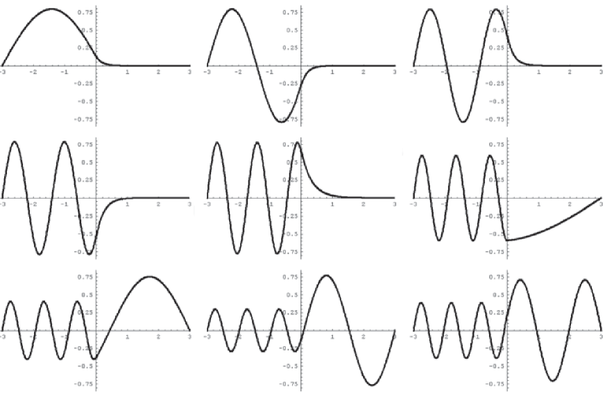
Figure 1: The first nine wave functions for the asymmetric infinite square well. In all of the images $\hbar=2m=1$, $V_{0}=33$, and $a=b=3$.

Eq. (14) can then be used to determine the allowed energy eigenstates since $k$ and $\kappa$ are both related to the energy via Eqs. (5) and (8). As an example of a typical set of position-space wave functions, in Figure 1 we have chosen $V_{0}=33$ and $\hbar=2m=1$ to visualize these states (properly normalized).

For the $E>V_{0}$ case, we find that the wave function in each region is

$$\psi_{\textrm{\tiny{I}}}(x)=A\sin(k[x+a])\;,$$ (15)

and

$$\psi_{\textrm{\tiny{II}}}(x)=C\sin(q[x-b])\;,$$ (16)

and again by matching these two pieces of the wave function at $x=0$, we find the energy-eigenvalue condition:

$$q\tan(ka)=-k\tan(qb)\;.$$ (17)

For $E>V_{0}$, the wave functions of the AISW have some interesting features as shown in Figure 1. For the first five states, corresponding to $E<V_{0}$, the wave function is mostly confined to the left half of the well. As the energy increases above the step height, as shown by the remaining states in Figure 1, the wave function now extends over the entire well with a noticeable change in ‘wiggliness’ and amplitude across the middle of the well. As was pointed out in robinett_asymmetric , there are also special cases (that occur for much higher energy states with these parameters, and are not shown) in which there is an antinode at $x=0$ which yields the same amplitude for the wave function across the well.

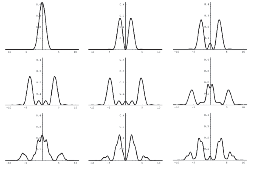
Figure 2: The first nine probability densities in momentum space for the asymmetric infinite square well corresponding to the same parameters as in Figure 1.

The same states shown in Figure 1 in position space are shown in Figure 2 in momentum space visualized using the momentum-space probability density. For the states with $E<V_{0}$, we note two peaks ($p=\pm\hbar k$ where $k$ is defined by Eq. (5)) in the probability density that get farther apart as the energy, and hence the momentum, increases. For the states with $E>V_{0}$, four peaks ($p=\pm\hbar q$ and $p=\pm\hbar k$ where $q$ and $k$ are defined by Eqs. (7) and (5), respectively) arise with the two peaks associated with the smaller momentum values ($p=\pm\hbar q$) having a noticeably larger probability than the two peaks associated with the larger momentum values ($p=\pm\hbar k$), as expected from classical time-spent arguments.

IV The Zero-curvature Solution

For $E=V_{0}$, the wave function in each region is

$$\psi_{\textrm{\tiny{I}}}(x)=A\sin(k[x+a])\;,$$ (18)

and

$$\psi_{\textrm{\tiny{II}}}(x)=C[x-b]\;,$$ (19)

and by matching these two pieces of the wave function at $x=0$, we find:

$$A\sin(ka)=-Cb\;,$$ (20)

and

$$kA\cos(ka)=C\;.$$ (21)

By dividing Eq. (20) by Eq. (21) and simplifying, we have the energy-eigenvalue condition:

$$\tan(ka)=-kb\;,$$ (22)

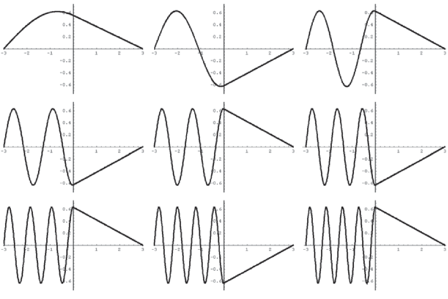
Figure 3: Nine zero-curvature wave functions with quantum numbers $n=1$ through $n=9$ for asymmetric infinite square wells with $a=b=3$ and different values of $V_{0}$ that satisfy Eq. (22). In all of the images $\hbar=2m=1$.

and since $E=V_{0}$, Eq. (22) is also a condition on $V_{0}$: $\tan(\sqrt{{\scriptstyle{2mV_{0}/\hbar^{2}}}}\,a)=-\sqrt{{\scriptstyle{2mV_{0}/\hbar^{2}}}}\,b$ . Zero-curvature solutions are, therefore, only possible for special AISWs with suitable values of $V_{0}$, $a$, and $b$, and the quantum number, $n$. It is easy to conclude that for an AISW, there exists either one or (more likely) no zero-curvature states in the energy spectrum. For example, in an AISW with $a=b=3$ and $\hbar=2m=1$, we find that zero-curvature states occur with: $V_{0}=0.457318\;(n=1),\;2.682149\;(n=2),\;7.073234\;(n=3),13.654351\;(n=4),\;22.427917\;(n=5),\;33.394444\;(n=6),\;46.55409\;(n=7),\;61.906917\;(n=8)$,  79.452954 (n = 9). The allowed zero-curvature wave functions for $n=1$ through $n=9$ with $a=b=3$ and the special $V_{0}$ values given above are shown in Figure 3.

If we consider the wave functions in Region II with the limiting cases in which $\kappa\rightarrow 0$ and $q\rightarrow 0$, we find that, $\psi_{{\textrm{\tiny{II}}}\,{\scriptscriptstyle{(E<V_{0})}}}(x)=\psi_{{\textrm{\tiny{II}}}\,{\scriptscriptstyle{(E>V_{0})}}}(x)\approx\psi_{{\textrm{\tiny{II}}}\,{\scriptscriptstyle{(E=V_{0})}}}(x)$. However, we must be careful not to assume this means that $\lim_{\kappa\rightarrow 0}\,\psi_{{\textrm{\tiny{II}}}\,{\scriptscriptstyle{(E<V_{0})}}}(x)$ and $\lim_{q\rightarrow 0}\,\psi_{{\textrm{\tiny{II}}}\,{\scriptscriptstyle{(E>V_{0})}}}(x)$ always give valid solutions to the $E=V_{0}$ case. They do not. Only in the cases where we have already tuned the potential energy well to yield a wave function energy of $E=V_{0}$ does taking the limit of the $E>V_{0}$ and $E<V_{0}$ wave functions yield the exact zero-curvature solution.

V Position-space Probability Distributions

While Eq. (18) and Eq. (19) give the wave function in each region, they must still match at $x=0$ and therefore we use Eq. (20) to yield

$$\psi(x)=\left\{\begin{array}[]{ll}A\sin[(k(x+a)]&\mbox{for $-a\leq x\leq 0$}\\ -A\frac{\sin(ka)}{b}(x-b)&\mbox{for $0\leq x\leq+b$}\end{array}\right.$$ (23)

for $\psi_{\textrm{\tiny{I}}}(x)$ and $\psi_{\textrm{\tiny{II}}}(x)$, apart from normalization. To normalize we require that

$$\!\!\!\!\!\!\!\!\!\!\!\!\!\!\!\!\!\!\!\!\!\!\!\!|\psi(x)|^{2}\,dx=A^{2}\int_{-a}^{0}\sin^{2}[(k(x+a)]\,dx+\left(\frac{A\sin(ka)}{b}\right)^{2}\int_{0}^{+b}(x-b)^{2}\,dx=1\;,$$ (24)

and we therefore find that

$$A=\left[\,\frac{a}{2}\left(1-\frac{\sin(2ka)}{2ka}\right)+\frac{b\sin^{2}(ka)}{3}\,\right]^{-1/2}\;.$$ (25)

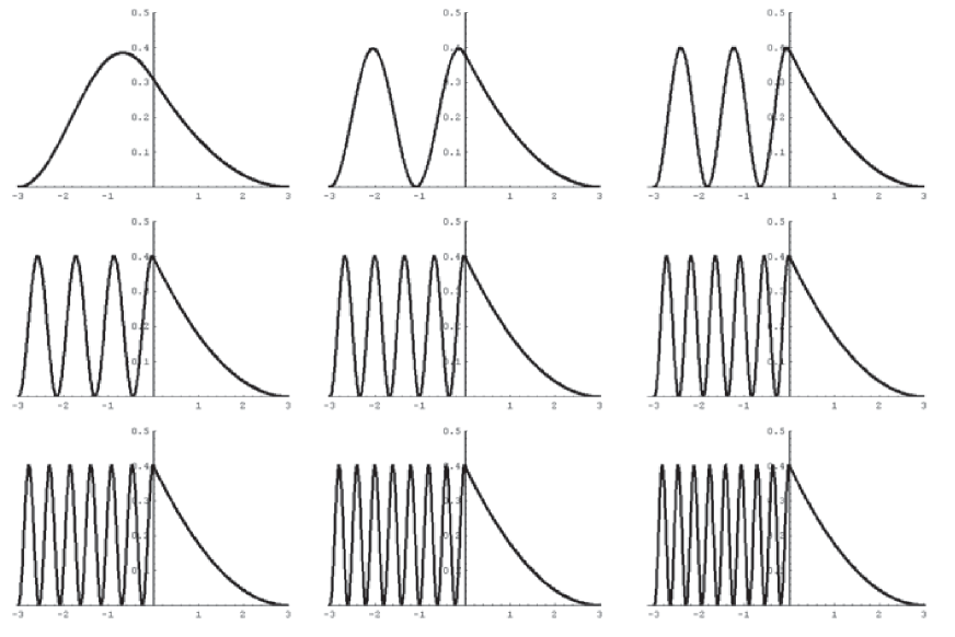
Figure 4: The probability densities for zero-curvature wave functions ($n=1$ through $n=9$) for the same nine wells used in Figure 3.

Shown in Figure 4 are the normalized probability densities for the zero-curvature states ($n=1$ through $n=9$) for the same nine wells used in Figure 3.

We also find by direct integration that the distribution of probability in the two regions is

$$\!\!\!\!\!\!\!\!\!\!\!\!\!\!\!\!\!\!\!\!\!\!\!P_{{\textrm{\tiny{I}}}}=\frac{a\left(1-\sin(2ka)/2ka\right)}{2[\,\frac{a}{2}(1-\sin(2ka)/2ka)+b\sin^{2}(ka)/3\,]}=A^{2}\left[\frac{a}{2}\left(1-\frac{\sin(2ka)}{2ka}\right)\right]\;,$$ (26)

and

$$\!\!\!\!\!P_{\textrm{\tiny{II}}}=\frac{b\,\sin^{2}(ka)}{3[\,\frac{a}{2}(1-\sin(2ka)/2ka)+b\sin^{2}(ka)/3\,]}=A^{2}\left[\frac{b\,\sin^{2}(ka)}{3}\right]\;.$$ (27)

We can analyze these results by noticing that as $n$ increases for the zero-curvature solution, Eq. (22) implies that $k\rightarrow\frac{(2n-1)\pi}{2a}$; this in turn yields $\sin(ka)\approx\pm 1$ (and therefore $\sin^{2}(ka)\approx 1$) and $\sin(2ka)\approx 0$. Eq. (26) and Eq. (27) reduce to $P_{\textrm{\tiny{II}}}\approx\frac{3a}{(3a+2b)}$ and $P_{\textrm{\tiny{II}}}\approx\frac{3b}{(3a+2b)}$, respectively, for large $n$. In the case where $a=b$, such as in all of the Figures, these equations yield $P_{{\textrm{\tiny{I}}}}\approx 0.6$ and $P_{\textrm{\tiny{II}}}\approx 0.4$. This approximation is already accurate to within 0.5% for the $n=6$ zero-curvature state and is borne out by Figure 4.

VI Momentum-space Probability Distributions

The zero-curvature wave functions in momentum space are straightforward to calculate from the position-space wave functions via the Fourier transformation:

$$\phi(p)=\frac{1}{\sqrt{2\pi\hbar}}\int_{-a}^{+b}\psi(x)\,e^{-ipx/\hbar}\,dx\;,$$ (28)

and by using the wave function in Eq. (23), we have

$$\phi(p)= \frac{A}{2i\sqrt{2\pi\hbar}}\,\int_{-a}^{0}\,\left(\,e^{ik(x+a)}-e^{-ik(x+a)}\,\right)\,e^{-ipx/\hbar}\;dx$$ (29)

$$-\frac{A\sin(ka)}{b\sqrt{2\pi\hbar}}\,\int_{0}^{+b}\,(x-b)\,e^{-ipx/\hbar}\,dx\;.$$

We can define these terms such that $\phi(p)\equiv\phi_{(+)}(p)+\phi_{(-)}(p)+\phi_{(0)}(p)$ where the $\phi_{(\pm)}(p)$ wave functions come from the $\exp[i(\mp k-p/\hbar)x]$ terms integrated over the left side of the well, and the $\phi_{(0)}(p)$ wave function comes from the linear term integrated over the right side of the well. The explicit expressions are given by

$$\!\!\!\!\!\phi_{(\pm)}(p)=\pm\frac{A}{\sqrt{2\pi\hbar}}\left(\frac{ai}{2}\right)e^{\mp ika}e^{+i(p\pm\hbar k)a/2\hbar}\left[\frac{\sin[(p\pm\hbar k)a/2\hbar]}{(p\pm\hbar k)a/2\hbar}\right]\;,$$ (30)

and

$$\phi_{(0)}(p)=\frac{A}{\sqrt{2\pi\hbar}}\left(\frac{\hbar^{2}\sin(ka)}{bp^{2}}\right)\left[1-ipb/\hbar-e^{-ipb/\hbar}\right]\;.$$ (31)

From these forms, it is clear that as the quantity $ka$ increases, the momentum-space wave functions become more noticeably peaked at $p=\pm\hbar k$ and $p=0$.

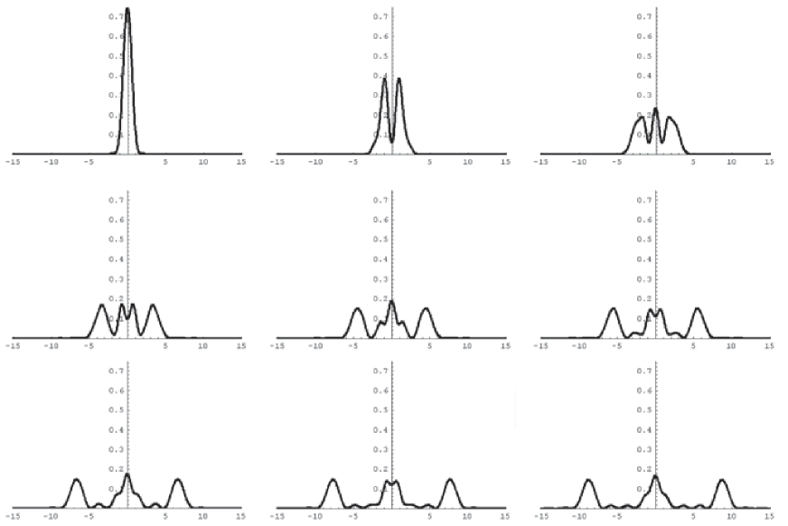
Figure 5: The zero-curvature probability densities in momentum space ($n=1$ through $n=9$) for the same nine wells used in Figure 3.

In Figure 5, we visualize the probability density in momentum space for the zero-curvature states ($n=1$ through $n=9$) for the same nine wells used in Figure 3.

Using these results, it is also easy to show that

$$\int_{-\infty}^{+\infty}|\phi_{(+)}(p)|^{2}\,dp=\int_{-\infty}^{+\infty}|\phi_{(-)}(p)|^{2}\,dp=A^{2}\left(\frac{a}{4}\right)\;,$$ (32)

$$\int_{-\infty}^{+\infty}|\phi_{(0)}(p)|^{2}\,dp=A^{2}\left(\frac{b\sin^{2}(ka)}{3}\right)\;,$$ (33)

$$\!\!\!\!\!\!\!\!\!\!\!\int_{-\infty}^{+\infty}\left[\phi_{(-)}^{*}(p)\,\phi_{(+)}(p)+\phi_{(-)}(p)\,\phi_{(+)}^{*}(p)\right]\,dp=-A^{2}\left(\frac{a\sin(2ka)}{4ka}\right)\;,$$ (34)

and

$$\!\!\!\!\!\!\!\!\!\!\!\!\!\!\!\!\int_{-\infty}^{+\infty}\left[\phi_{(0)}^{*}(p)\,\phi_{(+)}(p)+\phi_{(+)}^{*}(p)\,\phi_{(0)}(p)+\phi_{(0)}^{*}(p)\,\phi_{(-)}(p)+\phi_{(-)}^{*}(p)\,\phi_{(0)}(p)\right]\,dp=0\;,$$ (35)

where $A$ was previously defined in Eq. (25).

We first note that the position of the maxima of the central ‘peak’ alternates between a single peak at $p=0$ and two peaks at $p=\pm\alpha$ for odd and even values of $n$, respectively. For $p\approx 0$, the numerical value of the cross terms in the momentum-space probability density, the integrand in Eq. (35), alternates in sign as a function of $n$, thereby alternating constructive and destructive interference with the direct term, $|\phi_{(0)}(p)|^{2}$, as a function of $n$. The effect of these cross terms in the momentum-space probability density is therefore evident in the alternating position of the maximum of the central ‘peak,’ despite the fact that these terms do not yield any overall contribution to the probability as shown by Eq. (35).

Also note that the amount of probability in the various ‘peaks’ is directly comparable to the probabilities of being in the left or right regions of the well. We can easily make these assignments by noticing that the momentum-space probability of measuring the particle with $p\approx 0$ is $A^{2}b\sin^{2}(ka)/3$, which corresponds to the probability of being localized in the right side of the well since the probabilities calculated in Eq. (27) and Eq. (33) are identical. We can similarly compare the momentum-space probability for the $p\approx\pm\hbar k$ peaks to the probability of the particle being localized in the left side of the well, again finding that these are identical.

Given our well parameters, for large $n$ we find a momentum distribution that approaches 30% for the left peak (corresponding to a negative momentum in the left side of well), 40% for the central peak (corresponding to zero momentum in right side of well), and 30% for the right peak (corresponding to a positive momentum in the left side of well), again agreeing with the 60%-40% split in the position-space probability for the left and right regions of the well.

VII Conclusion

We have outlined the conditions in which an asymmetric infinite square well, and other piecewise-constant potential wells, can have a valid zero-curvature bound-state wave function. These position-space wave functions, and their momentum-space counterparts, are easily determined and visualized. They have readily calculable probability relationships which allow a direct comparison between the position- and momentum-space probabilities for each region of the well. Other infinite square well extensions, such as infinite well plus Dirac delta function cases zc_paper , can also exhibit zero-curvature solutions for the right well parameters. A more general analysis of these cases is straightforward, and will be addressed elsewhere other_paper .

Zero-curvature states can also serve an important pedagogical purpose as a way to easily extend the standard treatment of the AISW and other piecewise-constant potential wells. These special cases help further elucidate the connection between the potential energy function, the quantized energy eigenvalue, and the resulting form of the wave function in one-dimensional quantum-mechanical systems. While zero-curvature solutions are an intuitively natural interpolation between the much more frequently discussed oscillatory and tunneling solutions, the unfamiliar mathematical form of the one-dimensional Schrödinger equation in Eq. (11) for these parameters does catch many students by surprise.

A recent (unintentional) educational experiment, where first-year graduate students in physics were asked to consider just such a problem, showed that less than 20% could successfully find the linear solution in Eq. (11) and the resulting energy-eigenvalue condition in Eq. (22) on an exam. The most common mistake among these students, as is often seen in such physics education trials, was an attempt to fit ‘standard’ solutions (in this case those in Eq. (9) and Eq. (10)) to this slightly different situation. Having as wide an array of example problems allows instructors to better probe and shape student understanding of quantum-mechanical bound-state problems rick_qmvi .

In addition, the procedures we have outlined can be used to determine specifications for quantum wells, like those used in Ref. coherent_charge , so zero-curvature wave functions can be experimentally observed and their unique properties exploited. Such zero-curvature states are of interest because they may enhance scattering of wave packets in these special asymmetric infinite square wells sprung . This is yet another example of the experimental realization of ‘designer’ quantum wave functions meekhof .

- (1) Krane K S 1997 Modern Physics, 2nd edn (New York; John Wiley and Sons) 172
- (2) Morrison M A 1990 Understanding Quantum Physics: A User’s Manual (Upper Saddle River, New Jersey: Prentice Hall) 364-371, 377-379, 402-403
- (3) Robinett R W 1997 Quantum Mechanics: Classical Results, Modern Systems, and Visualized Examples (New York: Oxford) 120-122
- (4) Harrison P 2000 Quantum Wells, Wires, and Dots: Theoretical and Computational Physics (Chichester: Wiley and Sons) 47-49
- (5) Bonvalet A, Nagle J, Berger V, Migus A, Martin J-L, and M. Joffre M 1996 Femtosecond infrared emission resulting from coherent charge oscillations in quantum wells Phys. Rev. Lett. 76 4392-4395
- (6) Doncheski M A and Robinett R W 2000 Comparing classical and quantum probability distributions for an asymmetric well Eur. J. Phys. 21 217-228
- (7) Bowen M and Coster J 1980 Infinite square well: A common mistake Am. J. Phys. 49 80-81
- (8) Yinji L and Zianhuai H 1986 A particle ground state in the infinite square well Am. J. Phys. 54 738
- (9) Belloni M, Doncheski M A, and Robinett R W 2005 Zero-curvature solutions of the one-dimensional Schrödinger equation; Accepted for publication to Physica Scripta
- (10) Sakurai J J 1994 Modern quantum mechanics, Revised Edition (New York: Addison-Wesley) Section 7.7
- (11) Blatt J M and Weisskopf V F 1952 Theoretical Nuclear Physics (New York: John Wiley and Sons) Sections 2.2-2.3
- (12) Gilbert L P, Belloni M, Doncheski M A, and Robinett R W 2005 Piecewise zero-curvature solutions of the one-dimensional Schrödinger equation; To be submitted for publication
- (13) Cataloglu E and Robinett R 2002 Testing the development of student conceptual and visualization uderstanding in quantum mechanics through the undergraduate career Am. J. Phys. 70 238-251
- (14) Sprung D W L, Wu H, and Martorell J 1996 Poles, bound states, and resonances illustrated by the square well potential Am. J. Phys. 64 136-144
- (15) Meekhof D M, Monroe C, King B E, Itano W M, and Wineland D J 1996 Generation of nonclassical motional states of a trapped atom Phys. Rev. Lett. 76 1796