The limits of the rotating wave approximation in the electromagnetic field propagation in a cavity

Abstract

We consider three two-level atoms inside a one-dimensional cavity, interacting with the electromagnetic field in the rotating wave approximation (RWA), commonly used in the atom-radiation interaction. One of the three atoms is initially excited, and the other two are in their ground state. We numerically calculate the propagation of the field spontaneously emitted by the excited atom and scattered by the second atom, as well as the excitation probability of the second and third atom. The results obtained are analyzed from the point of view of relativistic causality in the atom-field interaction. We show that, when the RWA is used, relativistic causality is obtained only if the integrations over the field frequencies are extended to $-\infty$; on the contrary, noncausal tails remain even if the number of field modes is increased. This clearly shows the limit of the RWA in dealing with subtle problems such as relativistic causality in the atom-field interaction.

1 Introduction

The propagation of electromagnetic signals has been a subject of investigation since the beginning of the quantum theory of the electromagnetic field. In the last years this subject has received much attention in the framework of rigorous proofs of relativistic causality in the atom-field interaction [1, 2, 3, 4], of the recently observed slow light propagation [5] and of the possibility of superluminal propagation of light [6].

Recently, the propagation and the scattering of a photon spontaneously emitted by an atom in a one-dimensional cavity has been investigated using the rotating wave approximation (RWA) [7]. This approximation consists in neglecting non-energy conserving terms in the Hamiltoniam, and the potential dangers of this approximation in terms of the causal behaviour of the physical system considered are well known [8, 3]. Quite frequently, the effect of the RWA seems to be compensated by the extension to $-\infty$ of the integrations in the frequency of the field modes, as in the original Fermi model description of causality in the excitation transfer between two atoms, one of which initially excited [9, 10, 11]. Yet, this is in any case conceptually unsatisfactory for a subtle problem such as relativistic causality, and much effort has been dedicated to the inclusion of the counterrotating terms in order to have a rigorous proof of relativistic causality in quantum electrodynamics [4, 12].

In this letter we consider the same system considered by Purdy et al. in [7]. This system consists of three two-level atoms inside a one-dimensional cavity, interacting with the electromagnetic field in the RWA. We show numerically that the causal behaviour obtained in [7] (using the RWA) indeed derives from an extension to $-\infty$ of the frequency integrations; this extension, however, has no physical justification since it makes the Hamiltonian unbounded from below, and this is in general a fundamental point for the causality problem, as pointed out by Hegerfeldt [13]. We show that even if the Hamiltonian is bounded from below, noncausal terms in the field propagation are present when the rotating wave approximation is used; these terms do not vanish when the number of field modes is increased. This explicitly shows that the RWA is not an appropriate approximation for dealing with problems of relativistic causality in matter-radiation systems, and that the counterrotating terms should be included.

Our system is the same as in [7]: it consists of three two-level atoms, named 1, 2, 3, in a one-dimensional cavity. The cavity has length $L$, with two parallel plates at $x=0$ and $x=L$, and the positions of the atoms 1, 2, 3 are $L/4$, $L/2$ and $3L/4$, respectively. In the Coulomb gauge and multipolar coupling scheme, within dipole approximation and using the rotating wave approximation, the interaction of the three atoms with the radiation field is described by the following Hamiltonian (with units such that $\hbar=1$)

$$H=\sum_{j=1}^{3}\omega_{j}S_{j}^{z}+\sum_{n}\omega_{n}a_{n}^{\dagger}a_{n}+\sum_{n}\sum_{j=1}^{3}\left(g_{jn}a_{n}S_{j}^{+}+g_{jn}^{\star}a_{n}^{\dagger}S_{j}^{-}\right)$$ (1)

where index $n=1,2,3,\ldots$ denotes the field modes of the cavity and $j=1,2,3$ denotes the atoms. $a_{n},a_{n}^{\dagger}$ are the annihilation and creation operators of the n-th mode, $S_{j}^{\pm},S_{j}^{z}$ are the pseudospin operators of the atom $j$, and

$$g_{jn}=\Omega_{j}\sin\frac{n\pi x_{h}}{L}\hskip 5.0pt;\hskip 15.0pt\Omega_{j}=\mu_{j}\sqrt{\frac{\omega_{j}}{2\epsilon_{0}L}}$$ (2)

where $\omega_{j}$ is the transition frequency of atom $j$ and $\mu_{j}$ is its electric dipole moment. In the expression of the coupling constant the near-resonance approximation $\omega_{n}\simeq\omega_{j}$ has been used.

We wish to stress that, because we are describing our system in the multipolar coupling scheme, the field operator that we calculate, the momentum conjugate to the vector potential, is the transverse displacement field ${\bf D}_{\perp}({\bf r})$. This operator, outside the sources, coincides with the total electric field ${\bf E}({\bf r})$. This is an essential point, because ${\bf E}({\bf r})$ satisfies a retarded wave equation, and thus it is expected to manifest causal propagation in space. On the contrary, when the minimal coupling scheme is used, the field operator conjugate to the vector potential is the transverse electric field ${\bf E}_{\perp}({\bf r})$, which is not a retarded operator; in fact, the source term in the corresponding Maxwell equation is the transverse current density, which is not localized in space for atomic systems [14].

Our initial state is the state with atom 1 excited, atoms 2 and 3 in their ground states and the field in the vacuum state, that is $\mid e,g,g,0_{k}\rangle$. In the RWA the only states participating to the evolution of the initial state are, with an obvious meaning of the symbols, $\mid g,e,g,0_{n}\rangle$, $\mid g,g,e,0_{n}\rangle$, $\mid g,g,g,1_{n}\rangle$. Thus we can write the general state at time $t$ as the following superposition

$$\mid\psi(t)\rangle = c_{1}(t)\mid e,g,g,0_{n}\rangle+c_{2}(t)\mid g,e,g,0_{n}\rangle$$ (3)

$$+ c_{3}(t)\mid g,g,e,0_{n}\rangle+\sum_{n}b_{n}(t)\mid g,g,g,1_{n}\rangle$$

The Schrödinger equation gives the following set of coupled differential equations for the coefficients

$$\dot{c}_{j}(t) = -i\left(\omega_{j}c_{j}(t)+\sum_{n}g_{jn}b_{n}(t)\right)$$ (4)

$$\dot{b}_{n}(t) = -i\left(\omega_{n}b_{n}(t)+\sum_{j}^{3}g_{jn}^{\star}c_{j}(t)\right)$$ (5)

We assume that the atoms 1 and 3 have the same transition frequency, $\omega_{1}=\omega_{3}$, and we indicate with $\delta=\omega_{1}-\omega_{2}$ the detuning of atom 2 compared with atoms 1 and 3. We also put $L/c=1$, which means using as the unit time the time taken by the light to cross the cavity.

Approximate analytical solutions of these equations have been obtained [15], using a method based on Laplace transforms [16]. We have obtained numerical solutions of these equations. We integrate numerically the set of differentially equations (4,5) with the Adams-Moulton-Bashfort method [17, 18]. This multistep method is an algorithm more sophisticated than the Runge-Kutta method, typically used for this kind of problems, allowing to obtain more accurate results and to use a much larger number of cavity modes. In order to facilitate comparison of our numerical results with the analytical results obtained in [15], we shall adopt the same numerical values of the detuning $\delta$ and of the atomic decay rates $\gamma_{j}=\mid\Omega_{j}\mid^{2}$. Therefore, we use $\gamma_{1}=1$, $\gamma_{2}=16$, $\gamma_{3}=256$ and $\delta=4$ (in our units).

We calculate the expectation value of the square of the electric field, which is proportional to the electric part of the field energy density, given by (zero-point terms have been neglected)

$$\langle E^{2}(x,t)\rangle=2\frac{\omega_{1}}{L}\left|\sum_{n}b_{n}(t)\sin\left(\frac{\omega_{n}x}{c}\right)\right|^{2}$$ (6)

Our first numerical calculation involves a set of equally spaced field modes, symmetric with respect to the resonance frequency of the first atom. This simulates an integration extended from $-\infty$ to $+\infty$, therefore a field Hamiltonian not bounded from below (as that used in [7]). In this paper we report the results of two numerical calculations: the first uses $10^{4}$ modes, 5000 above and 5000 below the atomic frequency; the second uses $2\cdot 10^{4}$ modes, $10^{4}$ above the atomic frequency and $10^{4}$ below. We then compare the results obtained with those of an analogous numerical calculation in which the field modes are not symmetric with respect to the atomic frequency, and only the upper cut-off is increased with increasing the number of the field modes; this second case simulates a field Hamiltonian bounded from below. This comparison allows us to understand the role of the RWA in the behaviour of our system, in particular from the point of view of relativistic causality.

Fig. 1 shows $\langle E^{2}(x,t)\rangle$ at $t=0.25$ when $10^{4}$ modes are used with a symmetric distribution around the transition frequency. A front in the propagation of the energy density is evident at $x=0.5$, as expected (the atom that emits the radiation is located at $x=0.25$); however, a zoom of Fig. 1 in the neighbourhood of $x=0.5$, given in Fig. 2, shows the presence of tails for $x>0.5$, blurring the front. Fig. 2 also shows the same expansion around $x=0.5$ when a larger number of modes is used ($2\cdot 10^{4}$), again with a symmetric configuration around the atomic frequency. An improvement of the behaviour from the point of view of causality is evident, with a manifest decrease of the tails for $x>0.5$. We have also obtained similar results for different times, showing that the front gets sharper when the number of field modes is increased, if the frequencies of the field modes are symmetric around the transition frequency of the atom. This suggests that the expected causal behaviour is indeed approached in the limit of an infinite number of field modes symmetrically distributed around $\omega_{1}$.

The behaviour is quite different when the number of field modes is increased in such a way that only the upper cut-off frequency increases but the lower cut-off frequency remains fixed (in this case the frequencies of the field modes are not symmetric with respect to the atomic transition frequency); this situation is intended to mimic the case in which the field modes extend from $0$ to $\infty$, and no extension to $-\infty$ is performed. Fig. 3 shows a zoom around $x=0.5$ of the square of the electric field at time $t=0.25$ for $10^{4}$, $2\cdot 10^{4}$ and $3\cdot 10^{4}$ modes. The figures indicate that, as the number of modes is increased, the envelop of the oscillations does not approximate a sharp front. The remaining tail gives a noncausal behaviour. This makes quite evident that the use of the rotating wave approximation with an Hamiltonian bounded from below does not give causality in the propagation of the electromagnetic fields, because noncausal tails persist, consistently with Hegerfeldt’s theorem.

Similar conclusions are reached by calculating $\mid c_{3}(t)\mid^{2}$, that is the excitation probability of atom 3. Causality requires that this probability should vanish for $t<0.5$. Fig. 4 shows our numerical results, and Fig. 5 a zoom around the causality time $t=0.5$ (with $10^{4}$ and $2\cdot 10^{4}$ modes), both with a symmetric configuration of the mode frequencies. We note that a sharper front is obtained when the number of the modes is increased. However, Fig. 6 shows the result for the non-symmetric configuration, in which only the upper cut-off frequency is increased with the field modes. It is evident from Fig. 6 that in this case the noncausal tails for $t<0.5$ do not decrease on the average as the number of the modes is increased.

We wish to conclude by stressing that our results clearly show the reason why recent results in the literature have obtained a causal behaviour of the atom-field interaction in a cavity within the rotating wave approximation. The point is that at the same time the frequency integration over the field modes was extended to $-\infty$ which permits to escape the conditions set by Hegerfeldt’s theorem by making the Hamiltonian unbounded from below, but which is physically unacceptable. In this paper, we have considered three two-level atoms, one excited and two in the ground state, inside a one-dimensional cavity, interacting with the electromagnetic radiation field in the RWA. We have calculated numerically the energy density of the electric field spontaneously emitted by the excited atom and scattered by the second atom, as well as the probability of excitation of the second and third atom. We have shown that, without the (arbitrary) extension of the field frequencies to $-\infty$ (frequently used in the literature), and which has no physical basis, noncausal tails are present both in the field propagation inside the cavity and in the atomic excitation probabilities, even when the number of the modes is increased. This underlines the potential dangers of the rotating wave approximation. In a forthcoming paper, we will explicitly show that the correct inclusion of the counter-rotating terms of the Hamiltonian, allows to obtain a better causal behaviour without any need of extending the frequency of the modes to $-\infty$.

The authors wish to thank P.P. Corso for helpful comments and suggestions on the numerical calculations. This work was in part supported by the bilateral Italian-Belgian project on “Casimir-Polder forces, Casimir effect and their fluctuations” and the bilateral Italian-Japanese project 15C1 on “Quantum Information and Computation” of the Italian Ministry for Foreign Affairs. Partial support by Ministero dell’Università e della Ricerca Scientifica e Tecnologica and by Comitato Regionale di Ricerche Nucleari e di Struttura della Materia is also acknowledged.

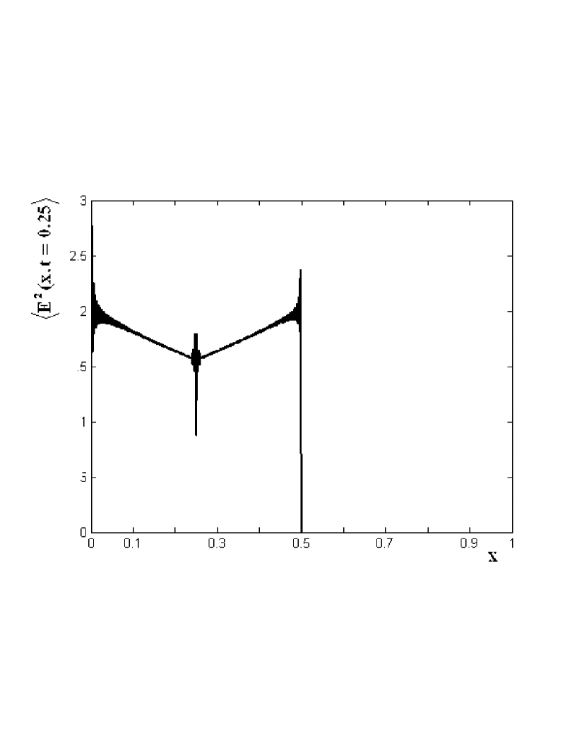
Figure 1: Average value of the square of the electric field $E^{2}(x,t)$ in arbitrary units at $t=0.25$, with $10^{4}$ field modes symmetrically distributed around the atomic transition frequency.

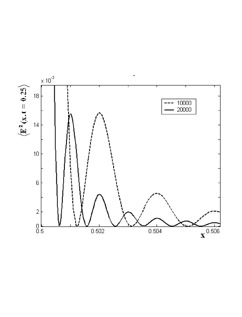
Figure 2: Average value of $E^{2}(x,t)$ in arbitrary units at $t=0.25$ in the neighbourhood of $x=0.5$. The dashed line is with $10^{4}$ modes of the field and the continuous line with $2\cdot 10^{4}$ modes (both with a symmetric mode distribution around the atomic transition frequency).

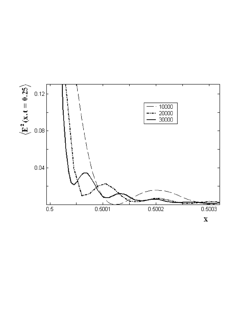
Figure 3: Average value of $E^{2}(x,t)$ in arbitrary units in the neighbourhood of $x=0.5$ at time $t=0.25$, with $10^{4}$ modes (dashed line), $2\cdot 10^{4}$ (dotted line) and $3\cdot 10^{4}$ (continuous line). The distribution of the field modes used here is not symmetric respect to the atomic transition frequency.

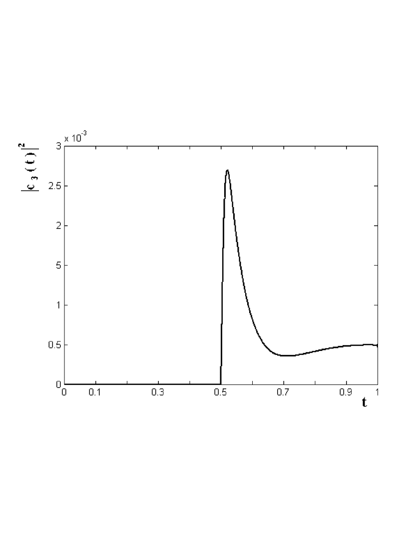
Figure 4: Excitation probability of atom 3, with a configuration of the field modes symmetric around $\omega_{1}$.

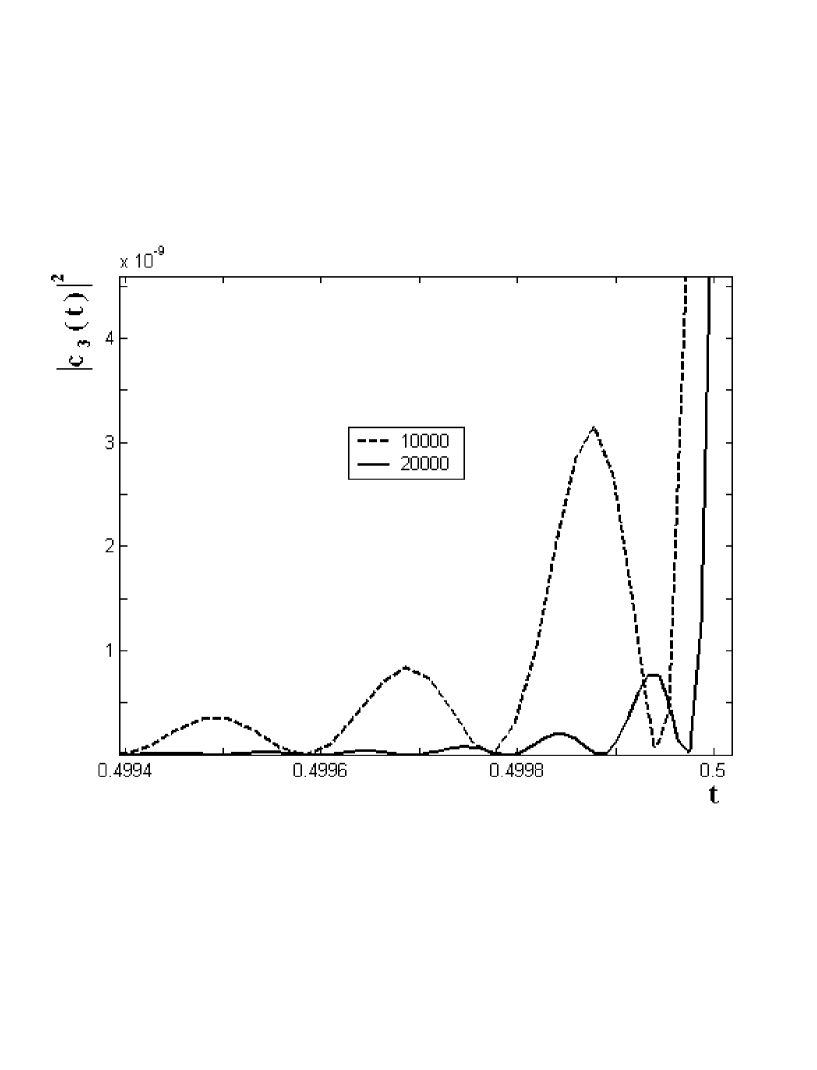
Figure 5: Zoom of Fig. 4: excitation probability of atom 3 with a symmetric configuration of the field modes, around the causality time $t=0.5$.

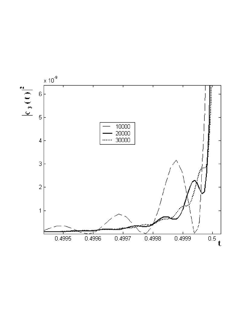
Figure 6: Zoom of the excitation probability of atom 3 around the causality time $t=0.5$, using a non-symmetric distribution of the field modes.

References

- [1] E.A. Power, T. Thirunamachandran, Phys. Rev. A 28, 2663 (1983)
- [2] P.R. Berman, Phys. Rev. A 69, 022101 (2004)
- [3] P.W. Milonni, D.F.V. James, H. Fearn, Phys. Rev. A 52, 1525 (1995)
- [4] G. Compagno, G.M. Palma, R. Passante, F. Persico, Chem. Phys. 198, 19 (1995)
- [5] L.V. Hau, S.E. Harris, Z. Dutton, C.H. Behroozi, Nature 397, 594 (1999)
- [6] R.Y. Chiao, Phys. Rev. A 48 R34 (1993)
- [7] T. Purdy, D.R. Taylor, M. Ligare, J. Opt. B: Quantum Semiclass. Opt. 5, 85 (2003)
- [8] A.K. Biswas, G. Compagno, G.M. Palma, R. Passante, F. Persico, Phys. Rev. A 42, 4291 (1990)
- [9] E. Fermi, Rev. Mod. Phys. 4, 87 (1932)
- [10] K. Ujihara, H.T. Dung, Phys. Rev. A 66, 053807 (2002)
- [11] Z. Haizhen, K. Ujihara, Opt. Comm. 240, 153 (2004)
- [12] E.A. Power, T. Thirunamachandran, Phys. Rev. A 56, 3395 (1995)
- [13] G.C. Hegerfeldt, Phys. Rev. Lett. 72, 596 (1994)
- [14] G. Compagno, R. Passante, F. Persico, Atom-Field Interactions and Dressed Atoms, Cambridge University Press, Cambridge 1995
- [15] T. Purdy, M. Ligare, J. Opt. B: Quantum Semiclass. Opt. 5, 289 (2003)
- [16] G.C. Stey, R.W. Gibberd, Physica 60, 1 (1972)
- [17] W.H. Press, S.A. Teukolsky, W.T. Vetterling, B.P. Flannery, Numerical Recipes in C: The Art of Scientific Computingm Cambridge University Press, Cambridge 1995
- [18] G. Wheatley, Applied Numerical Analysis, Addison-Wesley Publishing, Reading, Ma 1995