Persistent single-photon production by tunable on-chip micromaser with a superconducting quantum circuit

Abstract

We propose a tunable on-chip micromaser using a superconducting quantum circuit (SQC). By taking advantage of externally controllable state transitions, a state population inversion can be achieved and preserved for the two working levels of the SQC and, when needed, the SQC can generate a single photon. We can regularly repeat these processes in each cycle when the previously generated photon in the cavity is decaying, so that a periodic sequence of single photons can be produced persistently. This provides a controllable way for implementing a persistent single-photon source on a microelectronic chip.

I Introduction

Superconducting quantum circuits can behave like natural atoms and are also promising candidates of qubits for scalable quantum computing.YN05 Moreover, these circuits also show quantum optical effects and provide exciting opportunities for demonstrating quantum effects at macroscopic scales and for conducting atomic-physics experiments on a microelectronic chip (see, e.g., Refs. YN05, ; CHIO, ; YN03, ; YANG, ; YALE04, ; LIU04, ; ZAGO, ; LIU05, ; NANO, ).

Because of its fundamental importance in quantum communications, single-photon sources are crucial in both quantum optics and quantum electronics.REVIEW Single-photon sources can be achieved using quantum-dot-based devices (see, e.g., Ref. SPS, ), but their frequencies are not in the microwave regime required for superconducting qubits. Recently, there have been efforts to generate single photons by coupling a superconducting qubit to a superconducting resonator.YALE04 ; LIU04 ; MARI However, because of damping inside the resonator, the generated single photon can only persist for a very short time.

Here we show how to persistently produce steady microwave single photons by a tunable micromaser using a superconducting quantum circuit (SQC). The physical mechanism is as follows: The SQC acts like a controllable artificial atom (AA) and is placed in a quantum electrodynamic cavity. By taking advantage of the externally controllable state transitions, one can pump the AA to produce state population inversion for the two working levels. This population inversion is preserved by turning off the transition to the ground state, but when needed this transition can be switched on to generate a photon. Within the photon lifetime of the cavity, one can pump the superconducting AA to produce the state population inversion again for the next cycle of operations and then switch on the state transition when the photon generated in the previous cycle is decaying. By periodically repeating this cycle, one can generate single photons in a persistent way.

Steady-state photons can also be generated by a micromaser with natural atoms (see, e.g., Refs. MASER, and ORZ, ). However, in such a micromaser, there is a very small number of excited atoms among all atoms passing through the cavity and these excited atoms enter the cavity at random times. This will produce large fluctuations for the photon field of the cavity. For instance, an excited atom can enter the cavity long before or after the previously generated single photon decays. To overcome this problem, a state population inversion is prepared for the superconducting AA in each cycle and all the cycles are repeated periodically. Also, the cavity can be realized using an on-chip superconducting resonator so that both the SQC and the resonator can be fabricated on a chip. This might be helpful for transferring quantum information between superconducting qubits in future applications. Moreover, in contrast to the fixed difference between the two working energy levels in a natural atom, the level difference for the superconducting AA is tunable, providing flexibility for producing a single-photon source over a wider frequency region.

In Ref. BAR, , spontaneous and stimulated emission characteristics was investigated for a Josephson-junction-cavity system, but here we focus on the quantum electrodynamic effects in the strong-coupling regime for a superconducting AA in the on-chip cavity. Moreover, the circuit design in this approach provides an enhanced level of control that is desirable for producing a single-photon source.

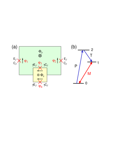
Figure 1: (Color online) (a) Schematic diagram of the superconducting artificial atom. A symmetric SQUID and two identical Josephson junctions with coupling energy $E_{J}$ and capacitance $C_{J}$ are placed in a superconducting loop pierced by an externally applied magnetic flux (green) $\Phi_{e}$. The two Josephson junctions in the symmetric SQUID have coupling energy $\gamma E_{J}$ and capacitance $\gamma C_{J}$, and the applied flux (yellow) threading through the SQUID loop is $\Phi_{s}$. Here we choose $\gamma=0.5$ and $E_{J}/E_{c}=100$, with $E_{c}=e^{2}/2C_{J}$ being the single-particle charging energy of the junction. (b) Transition diagram of a tunable artificial atom (i.e., a qutrit) used for the micromaser. A microwave field pumps the qutrit to make the transition $|0\rangle\longrightarrow|2\rangle$ (denoted as P) and another microwave field triggers the transition $|2\rangle\longrightarrow|1\rangle$ (denoted as T). With a state population inversion population inversion established for $|0\rangle$ and $|1\rangle$, the transition between $|0\rangle$ and $|1\rangle$ (denoted as M) is switched off to preserve the population inversion and, when needed, switched on to couple the AA with the cavity mode.

II Superconducting artificial atom

We consider an AA based on the SQC for the flux qubit.FLUX Instead, we use it as a qutrit involving the lowest three energy levels of the device. Also, the fourth and other higher levels are well separated and not populated. As shown in Fig. 1(a), in addition to two identical Josephson junctions, a symmetric SQUID is placed in the loop pierced by an external magnetic flux $\Phi_{e}$. This SQUID increases the external controllability of the quantum circuit by providing a tunable effective coupling energy: $\alpha E_{J}$ with $\alpha=2\gamma\cos(\pi\Phi_{s}/\Phi_{0})$, where $\Phi_{0}$ is the flux quantum.

The Hamiltonian of the system is

$$H=\frac{P_{p}^{2}}{2M_{p}}+\frac{P_{q}^{2}}{2M_{q}}+U(\varphi_{p},\varphi_{q}),$$ (1)

with

$$P_{i} \!=\! -i\hbar\frac{\partial}{\partial\varphi_{i}},\;\;\;\;i=p,q,$$

$$M_{p} \!=\! 2C_{J}(\Phi_{0}/2\pi)^{2},$$ (2)

$$M_{q} \!=\! \frac{1}{4}M_{p}(1+4\gamma).$$

The potential $U(\varphi_{p},\varphi_{q})$ is

$$U(\varphi_{p},\varphi_{q}) \!=\! 2E_{J}[1-\cos\varphi_{p}\cos(\pi f+\frac{1}{2}\varphi_{q})]$$ (3)

$$+2\gamma E_{J}[1-\cos(\pi f_{s})\cos\varphi_{q}],$$

where $\varphi_{p}=(\varphi_{1}+\varphi_{2})/2$ and $\varphi_{q}=(\varphi_{3}+\varphi_{4})/2$. The reduced fluxes $f_{s}$ and $f$ are given by

$$f_{s}=\frac{\Phi_{s}}{\Phi_{0}}\,,\;\;\;f=\frac{\Phi_{e}}{\Phi_{0}}+\frac{f_{s}}{2}\,.$$ (4)

The operator $P_{k}$ and the phase $\varphi_{j}$ obey $[\varphi_{j},P_{k}]=i\hbar\delta_{jk}$, where $j,k=p,q$.

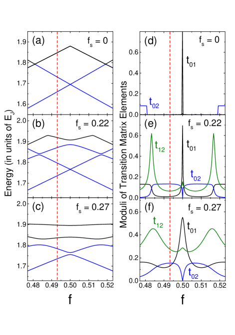
Figure 2: (Color online) (a)-(c) Energy levels of the superconducting artificial atom versus the reduced magnetic flux $f=\Phi_{e}/\Phi_{0}+f_{s}/2$ for $f_{s}(\equiv\Phi_{s}/\Phi_{0})=0$, $0.22$, and $0.27$, where only the lowest four energy levels ($E_{i}$, $i=0$ to 3) are shown. (d)-(f) Moduli of the transition matrix elements $|t_{ij}|$ (in units of $I_{c}\Phi_{w}^{(0)}$) versus the reduced flux $f$ for $f_{s}=0$, $0.22$, and $0.27$. Two vertical (red) dashed lines are plotted at $f=0.493$ as a guide to the eye.

To make a transition between two energy levels $E_{i}$ and $E_{j}$ of the superconducting AA, a microwave field

$$\Phi_{w}(t)=\Phi_{w}^{(0)}\cos(\omega_{ij}t+\theta)$$ (5)

is applied through the larger superconducting loop of the quantum circuit. For a weak microwave field, the time-dependent perturbation Hamiltonian is

$$H^{\prime}(t)=-I\Phi_{w}(t),$$ (6)

and the transition matrix element between states $|E_{i}\rangle$ and $|E_{j}\rangle$ is given by

$$t_{ij}=\langle E_{i}|\,I\,\Phi_{w}^{(0)}|E_{j}\rangle,$$ (7)

where

$$I=-I_{c}\cos\varphi_{p}\sin(\pi f+\frac{1}{2}\varphi_{q})$$ (8)

is the circulating supercurrent in the loop without the applied microwave field, and the critical current of the junction is defined as $I_{c}=2\pi E_{J}/\Phi_{0}$.

Figures 2(a)-2(c) display the dependence of the energy levels on the reduced flux $f$ for three different values of $f_{s}$. For a symmetric SQUID with $\gamma=0.5$, these values of $f_{s}$ give rise to an effective Josephson coupling energy $\alpha E_{J}$ with $\alpha=1$, $0.77$, and $0.66$, respectively. At $f_{s}=0$, the third and fourth energy levels become degenerate and other adjoining levels touch at the crossing points. When $f_{s}$ increases, this state degeneracy is removed and gaps develop at the crossing points, more pronounced for higher levels. In Figs. 2(d)-2(f), we show the moduli of the transition matrix elements $|t_{ij}|$ for the lowest three levels. At $f_{s}=0$, the transition matrix elements $t_{01}$, $t_{02}$ and $t_{12}$ become zero in a wider region around $f=0.5$. This means that the corresponding state transitions are forbidden. With $f_{s}$ increasing, these state transitions become allowed, but the modulus of each transition matrix element increases in a different manner. In contrast, $|t_{01}|$ for the state transition between the two lowest levels $E_{0}$ and $E_{1}$ increases slowly. Below we will explore these novel properties to implement a micromaser using a quantum circuit on a chip. Also, a superconducting ring containing only one Josephson junction can be used to achieve a qutrit (see, e.g., Ref. HANPRL, ), but it requires a relatively large loop inductance, which makes the qutrit more susceptible to the magnetic-field noise.

III Fast adiabatic quantum-state control and state population inversion

The state evolution of the superconducting AA depends on the external parameters. For two given quantum states $|E_{i}\rangle$ and $|E_{j}\rangle$, to have the evolution adiabatic, the nonadiabatic coupling $\langle E_{i}|\frac{d}{dt}|E_{j}\rangle$ and the energy difference $E_{i}-E_{j}$ should satisfy the condition (see, e.g., Ref. LIU05, ):

$$\left|\frac{\hbar\langle E_{i}|(d/dt)|E_{j}\rangle}{E_{i}-E_{j}}\right|\ll 1.$$ (9)

Here we change $f_{s}$ but keep the reduced flux $f$ unchanged. The adiabatic condition can be rewritten as

$$K_{ij}\left|\frac{df_{s}}{dt}\right|\ll 1,$$ (10)

where

$$K_{ij}=\left|\frac{\hbar\langle E_{i}|(\partial H/\partial f_{s})|E_{j}\rangle}{(E_{i}-E_{j})^{2}}\right|.$$ (11)

Figure 3 shows the quantities $K_{01}$ and $K_{12}$ as a function of the reduced flux $f$ for different values of $f_{s}$. For instance, in the vicinity of $f=0.493$ (vertical dashed lines in Fig. 2), $K_{01}\sim 0.2$ for $f_{s}=0.27$ [see Fig. 3(a)]. We can have

$$K_{01}\left(\frac{df_{s}}{dt}\right)\sim 0.02\ll 1$$

with $df_{s}/dt=0.1$ ns^-1, corresponding to a speed of changing $\Phi_{s}$, $d\Phi_{s}/dt\sim 0.1\Phi_{0}$ per ns. When $f_{s}=0.22$,

$$K_{01}\left(\frac{df_{s}}{dt}\right)\sim 0.02$$

for $df_{s}/dt=2$ ns^-1, and $d\Phi_{s}/dt$ can be much faster, to have the adiabatic condition satisfied by decreasing $f_{s}$. Also, around $f=0.493$, $K_{12}\sim 0.4$ for $f_{s}=0.27$ [see Fig. 3(b)]. When $df_{s}/dt=0.1$ ns^-1,

$$K_{12}\left(\frac{df_{s}}{dt}\right)\sim 0.04\ll 1,$$

implying that the adiabatic condition is satisfied. For a smaller $f_{s}$, $K_{12}$ decreases significantly and a much higher $d\Phi_{s}/dt$ can be used. This important property reveals that, at $f\sim 0.493$, one can adiabatically manipulate the quantum states $|0\rangle\equiv|E_{0}\rangle$ and $|1\rangle\equiv|E_{1}\rangle$ of the superconducting AA by quickly changing $f_{s}$ (e.g., $d\Phi_{s}/dt\gtrsim 0.1\Phi_{0}$ ns^-1) in the region of $0\leq f_{s}\lesssim 0.27$.

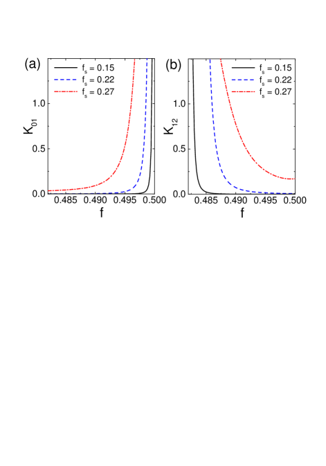
Figure 3: (Color online) The quantities (a) $K_{01}$ and (b) $K_{12}$ for the adiabatic condition versus the reduced flux $f$ for $f_{s}=0.15$, $0.22$, and $0.27$, respectively. Here we use $E_{J}=400$ GHz.

Below we manipulate the superconducting AA around our example case $f=0.493$ (the two vertical dashed lines in Fig. 2) by changing the flux $\Phi_{s}$ threading through the SQUID loop in three successive processes [see Fig. 1(b)]:

(i) Pumping process: First, the quantum circuit works at $f_{s}=0.22$. We constantly pump the superconducting AA with an appropriate microwave field to make the state transition $|0\rangle\longrightarrow|2\rangle\equiv|E_{2}\rangle$ for a period of time. Simultaneously, another microwave field is also used to trigger the transition $|2\rangle\longrightarrow|1\rangle$. For $f_{s}=0.22$, $|t_{01}|\approx 0.01$, $|t_{12}|\approx 0.07$, and $|t_{02}|\approx 0.13$. Because $|t_{01}|$ is about one order of magnitude smaller than $|t_{12}|$ and $|t_{02}|$, a population inversion between the two lowest states $|0\rangle$ and $|1\rangle$ can be readily achieved.

(ii) Preserving the population inversion: We decrease $f_{s}$ to $f_{s}=0$. Because $|t_{01}|$ now tends to zero, the transition $|1\rangle\longrightarrow|0\rangle$ is forbidden. For typical values $E_{J}/h=400$ GHz and $\Phi_{w}^{(0)}/\Phi_{0}\sim 1\times 10^{-4}$ (see Sec. V), the state population inversion can be preserved for a time $\sim 0.02$ s, much longer than the photon lifetime $\tau_{p}\sim 8$ $\mu$s of a cavity with quality factor $Q=10^{6}$.

(iii) Switching-on process: We increase $f_{s}$ to $f_{s}=0.27$ to turn on the transition $|1\rangle\longrightarrow|0\rangle$ with an appreciable probability (i.e., $|t_{01}|\approx 0.13$, which is one order of magnitude larger than $|t_{01}|\approx 0.01$ at $f_{s}=0.22$).

Here we emphasize that the two lowest energy levels are in resonance with the cavity mode when $f_{s}=0.27$. However, during the pumpimg, $f_{s}=0.22$. For this value of the reduced flux through the SQUID, the energy level difference between states $|0\rangle$ and $|1\rangle$ is appreciably different from that at $f_{s}=0.27$, so the two lowest levels at $f_{s}=0.22$ are very off-resonance with the cavity mode. Also, the level difference between $|0\rangle$ and $|2\rangle$ and that between $|1\rangle$ and $|2\rangle$ are very off-resonance with the cavity mode. Therefore, the qubit-cavity coupling is very weak during the pumping process, where we choose $f_{s}=0.22$ (instead of $f_{s}=0.27$, used for achieving strong qubit-cavity coupling).

IV Micromaser and single-photon source

IV.1 Interaction Hamiltonian

Let us place the superconducting AA in a quantum cavity, with the energy difference $E_{1}-E_{0}$ at $f=0.493$ and $f_{s}=0.27$ in resonance with the cavity mode. In the switching-on process, the superconducting AA acts as a two-level system and interacts with a single-mode quantized microwave field via Rabi oscillations, i.e., a coherent exchange of energy between them.

In the subspace with basis states $|1\rangle$ and $|0\rangle$, the circulating current can be written as

$$I=\frac{1}{2}(A-B)\sigma_{z}+(C\sigma_{+}+\rm{H.c.}),$$ (12)

where $A=\langle 1|I|1\rangle$, $B=\langle 0|I|0\rangle$, $C=\langle 1|I|0\rangle$, and $\sigma_{+}=|1\rangle\langle 0|$ is the raising operator for the states of the two-level system. The quantized microwave field in a cavity can be written as

$$\Phi_{w}=\Phi_{w}^{(0)}(a+a^{{\dagger}}),$$ (13)

where $a$ ($a^{{\dagger}}$) is the annihilation (creation) operator of photons of the cavity mode. In the rotating-wave approximation, $(C\sigma_{+}+\rm{H.c.})\Phi_{w}$ becomes $(t_{01}\sigma_{+}a+\rm{H.c.})$. Then, the interaction Hamiltonian (6) can be written as

$$H^{\prime}=-\frac{1}{2}(A-B)\Phi_{w}^{(0)}\sigma_{z}(a+a^{{\dagger}})-(t_{01}\sigma_{+}a+\rm{H.c.}).$$ (14)

The first term on the right-hand side of Eq. (14) only gives an effective contribution to the energy difference $E_{1}-E_{0}$ in the expression for the eigenvalues of the total Hamiltonian and it does not affect the Rabi oscillations. For the single-photon process we study, this contribution is a fixed value added to the energy difference $E_{1}-E_{0}$ and it can be included into the energy difference. Actually, this was explicitly shown for a charge qubit coupled via its SQUID loop to the cavity mode (see Ref. YN03, ). Therefore, one can only consider the Jaynes-Cummimgs term for the interaction Hamiltonian:

$$H^{\prime}=-\hbar g(\sigma_{+}a+{\rm H.c.}),$$ (15)

where

$$g=\frac{1}{\hbar}\,|t_{01}|.$$ (16)

In Eq. (15), we also ignore a phase factor that does not produce effects in our study.

Below we estimate the contribution of the first term on the right-hand side of Eq. (14). Usually, $A\sim-B\sim 0.5I_{c}$; in particular, $A=B=0$ at the degeneracy point $f=0.5$. Thus, we have

$$\frac{1}{2}(A-B)\Phi_{w}^{(0)}\sim 0.5I_{c}\Phi_{w}^{(0)}=\pi E_{J}({\Phi_{w}^{(0)}}/{\Phi_{0}}).$$

For a typical value of $\Phi_{w}^{(0)}/\Phi_{0}\sim 10^{-4}$ in our case (see Sec. V),

$$\frac{1}{2}(A-B)\Phi_{w}^{(0)}\sim 3\times 10^{-4}E_{J},$$

which is much smaller than the energy difference $E_{1}-E_{0}\sim 0.05E_{J}$ for $f=0.493$ and $f_{s}=0.27$. Thus, the first term on the right-hand side of Eq. (14) can also be ignored here, even if its contribution is not included into the energy difference.

IV.2 Photon statistics

We assume that the interaction between the cavity and the AA is in the strong-coupling regime, where the period $1/2g$ of the single-photon Rabi oscillations is much shorter than both the relaxation time of the two-level system and the average lifetime of the photon in the cavity. After an interaction time $\tau$, the quantum circuit turns to the pumping and population-inversion-preserving processes and it becomes ready for the next cycle of the three successive processes described above.

If the superconducting AA is switched on at the times $t_{i}$ to interact with the photons in the cavity, the time evolution of the density matrix $\rho$ of the cavity mode is governed by the map

$$\rho(t_{i}+\tau)=M(\tau)\rho(t_{i}),$$ (17)

where the gain operator $M(\tau)$ is defined as

$$M(\tau)\rho\! \!=\! \!{\rm Tr}_{a}\left[\exp\left(-\frac{i}{\hbar}H^{\prime}\tau\right)\rho\right.$$ (18)

$$\left.\otimes|1\rangle\langle 1|\exp\left(\frac{i}{\hbar}H^{\prime}\tau/\hbar\right)\right],$$

where ${\rm Tr}_{a}$ denotes the trace over the variables of the AA. Here we regularly switch on the superconducting AA by periodically repeating the cycle of the three successive processes described above.

With the cavity losses included, the dynamics of the density matrix $\rho$ is described by ORZ

$$\frac{d\rho}{dt}=r_{a}[M(\tau)-1]\rho-\frac{1}{2}r_{a}(M-1)^{2}\rho+L\rho.$$ (19)

In Eq. (19), $r_{a}$ is the switching-on rate for the superconducting AA. The operator $L$ describes the dissipation of the cavity photon due to a thermal bath:

$$L\rho\! \!=\! \!-\,\frac{1}{2}\kappa(n_{\rm th}+1)(a^{{\dagger}}a\rho+\rho a^{{\dagger}}a-2a\rho a^{{\dagger}})$$ (20)

$$\!-\,\frac{1}{2}\kappa n_{\rm th}(aa^{{\dagger}}\rho+\rho aa^{{\dagger}}-2a^{{\dagger}}\rho a),$$

where $n_{\rm th}$ is the average number of thermal photons in the cavity and $\kappa$ is the photon damping rate.

At steady state, $d\rho/dt=0$, which leads to a recursion relation for the steady photon number distribution $p_{n}=\langle n|\rho|n\rangle$ of the cavity mode:

$$p_{n+1}=\left\{\frac{n_{\rm th}}{n_{\rm th}+1}+\frac{2N_{t}S(n+1)[1+\frac{1}{2}S(n+1)]}{2(n_{\rm th}+1)(n+1)}\right\}p_{n}$$

$$~{}~{}~{}~{}~{}~{}~{}~{}~{}~{}-\frac{N_{t}S(n+1)S(n)}{2(n_{\rm th}+1)(n+1)}p_{n-1}\,,$$ (21)

with initial condition

$$p_{1}=\left\{\frac{n_{\rm th}}{n_{\rm th}+1}+\frac{2N_{t}S(1)[1+\frac{1}{2}S(1)]}{2(n_{\rm th}+1)}\right\}p_{0}\,,$$ (22)

where

$$S(n)=\sin^{2}(g\tau\sqrt{n}),\;\;\;n=0,1,2,\dots.$$ (23)

The quantity

$$N_{t}=\frac{r_{a}}{\kappa}$$ (24)

represents the number of cycles for switching on the superconducting AA during the photon lifetime of the cavity, and $p_{0}$ is determined by

$$\sum_{n=0}^{\infty}p_{n}=1.$$

Equation (21) is very different from the recursion relation for the atomic micromaser (see Ref. MASER, ), where all the excited atoms enter the cavity at random times:

$$(n_{\rm th}+1)np_{n}=[n_{\rm th}n+N_{t}S(n)]p_{n-1},$$ (25)

where

$$N_{t}=\frac{{\overline{r}}_{a}}{\kappa},$$ (26)

with ${\overline{r}}_{a}$ being the average injection rate of the excited atoms.

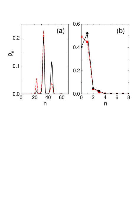
Figure 4: (Color online) Steady-state photon statistics for $n_{\rm th}=0.1$, and (a) $N_{t}=100$, $\tau_{\rm int}(\equiv g\tau\sqrt{N_{t}})=10\pi$; (b) $N_{t}=1$, $\tau_{\rm int}=1.4\pi$. These are results for a micromaser either using our quantum circuit (black solid lines) or using natural atoms, e.g., rubidium (red dashed lines).

In Fig. 4(a), we present the steady-state photon statistics for $N_{t}=100$. This statistics reveals an appreciable difference between the micromaser with natural atoms and that with a superconducting AA. Moreover, we show the steady-state photon statistics for $N_{t}=1$ [see Fig. 4(b)]. It is striking that the single-photon state has a probability at least one order of magnitude larger than multi-photon states. Figure 4(b) shows that the photon statistics of the atomic micromaser looks similar to that of the new proposed micromaser, but the results of the atomic micromaser are derived by approximating the injection rate of the atoms with an average value ${\overline{r}}_{a}$. Indeed, the injection rate of the atoms into the micromaser has a distribution, instead of a fixed value. This is in sharp contrast to an AA micromaser having a fixed rate $r_{a}$ of switching on the AA.

For the atomic micromaser, the excited atoms actually enter the cavity at random times and obey a Poissonian distribution. The number $n_{\rm ex}$ of the excited atoms has a larger variance to the average number $\overline{n}_{\rm ex}$: $\overline{\Delta n_{\rm ex}^{2}}=\overline{n}_{\rm ex}$, so larger fluctuations are expected for the photon field in the cavity. In contrast, in the micromaser using a SQC, the AA can be regularly switched on to interact with the photons in the cavity and the photon-field fluctuations are greatly reduced because $\overline{\Delta n_{\rm ex}^{2}}\sim 0$. Therefore, one can use the SQC micromaser to implement a persistent single-photon source with low-field fluctuations.

V Discussion

V.1 Experimentally accessible quantities

Let us consider a quasi-two-dimensional (2D) cavity, so that both the SQC and the cavity can be fabricated on the same chip. Moreover, the SQC is placed at an antinode of the cavity mode and the magnetic flux threads perpendicularly through the SQC loop. The quantized magnetic flux inside the SQC loop can be written as ORZ

$$\Phi_{w}=\Phi_{w}^{(0)}(a+a^{{\dagger}}),$$ (27)

with

$$\Phi_{w}^{(0)}=\left(\frac{h\nu}{\epsilon_{0}c^{2}Ah}\right)^{1/2}S_{q},$$ (28)

where $\nu$, $A$, $h$, and $S_{q}$ are the cavity frequency, the area of the quasi-2D cavity, the thickness of the cavity, and the area of the SQC loop, respectively. At $f=0.493$ and $f_{s}=0.27$, the numerical results in Fig. 2(c) give that $E_{1}-E_{0}\approx 0.05E_{J}$. When this level difference is in resonance with the cavity mode, the frequency of the cavity mode is $\nu=(E_{1}-E_{0})/h\approx 20$ GHz for a typical value of $E_{J}/h=400$ GHz; the wavelength is $\lambda\approx 1.5$ cm. Here, as an example, we use $A\sim(1.5~{}{\rm cm})^{2}$ and $h\sim 1$ $\mu$m for the quasi-2D cavity. Moreover, as shown in Ref. YNN, , the energy spectrum is nearly unchanged up to $\beta_{L}\equiv L/L_{J}\sim 0.1$, where the Josephson inductance is defined by $L_{J}=\Phi_{0}/2\pi I_{c}$. This gives a loop inductance $L\approx 40$ pH and the diameter of the loop is about $32$ $\mu$m. Then, we have

$$\Phi_{w}^{(0)}/\Phi_{0}\approx 1.1\times 10^{-4}.$$

Also, at $f=0.493$ and $f_{s}=0.27$, the numerical results in Fig. 2(f) give that $|t_{01}|=0.13I_{c}\Phi_{w}^{(0)}$. Using the values given above, we obtain

$$g=\frac{1}{\hbar}|t_{01}|\approx 218~{}{\rm MHz}.$$

For $N_{t}=1$ and $g\tau\sqrt{N_{t}}=1.4\pi$ [cf. Fig.4(b)], the corresponding interaction time $\tau$ for the AA to couple with the cavity mode in each cycle of operations is $\tau\approx 20$ ns. This value of $\tau$ is experimentally feasible because it is usually much shorter than the relaxation time $T_{1}$ of the flux qubit and also can easily be much shorter than the photon lifetime $\tau_{p}$ of an experimentally accessible high-Q superconducting cavity (e.g., $\tau_{p}\sim 8$ $\mu$s for $Q=10^{6}$).

In Ref. CHIO, , a relaxation time of about $1~{}\mu$s was measured for a flux qubit, away from the degeneracy point. For the JJs in that qubit, the ratio of the small to large junction is $\alpha=0.8$, which is close to $\alpha=0.77$ for Figs. 2(b) and 2(e) in this work. The longer relaxation time is due to a smaller transition matrix element $|t_{01}|$. In Fig. 2(e), $|t_{01}|$ is about $0.01$, when operating the flux qubit away from the degeneracy point (e.g., at $f=0.493$); in Ref. CHIO, , $\alpha=0.8$ and $|t_{01}|$ should be even smaller.

In order to achieve a strong-coupling regime, we consider the case in Figs. 2(c) and 2(f), where $\alpha=0.66$ and $|t_{01}|$ becomes larger than $0.1$ at $f=0.493$. Now, $|t_{01}|$ increases by more than one order of magnitude. Thus, because the relaxation time is proportional to $1/|t_{01}|^{2}$, the relaxation time should be shortened by two orders of magnitude, from about $1~{}\mu$s to about $10$ ns. In this case, the strong coupling between the flux qubit and cavity mode can be achieved, but the value of the relaxation time is comparable to the interaction time $20$ ns used for emitting a photon in the cavity.

Therefore, in our approach, we can use a novel way to change the parameter $\alpha$ by replacing the smaller junction with a tunable SQUID. Only when coupling the flux qubit with the cavity mode, we shift $\alpha$ to $\alpha=0.66$. When preparing the states of the flux qubit via realizing and preserving the state population inversion, we shift $\alpha$ to a smaller value, where the relaxation time can be long enough, even (in principle) arbitrarily long (in practice, it will not be infinitely long, but far longer than currently reachable). More importantly, we show that the process of changing $\alpha$ can be simultaneously adiabatic (so the state changes along the eigenstate) and fast enough (compared to the interaction time). This reveals its enhanced level of control and experimental feasibility.

V.2 Comparison with ordinary two-level system

In our proposal, the circuit design not only can either enhance or reduce the relaxation time for the transition from $|1\rangle$ to $|0\rangle$, but can also switch on and off this transition by changing the externally applied magnetic flux inside the SQUID loop. In particular, a state population inversion can be created via the third level and preserved for a long time. Moreover, when needed for generating a single photon, the SQC can be “turned on”, by changing an externally applied magnetic flux, to strongly couple to the cavity mode. These properties show that the circuit design provides an enhanced level of control, as compared with ordinary two-level systems.

If one wants to just observe the fundamental vacuum Rabi oscillations, it is suitable to manipulate only the two lowest levels of the SQC. However, when applied to the micromaser proposed here, it is very disadvantageous to only access the two lowest levels, since it is hard to maintain a state population inversion with only these two levels.

If one uses the two lowest levels of the SQC, in order to strongly couple the SQC to the cavity mode, the resonance point should be near the degeneracy point of the SQC, where the transition between $|1\rangle$ and $|0\rangle$ is the strongest. As shown in Ref. NTT, , one can first operate the SQC far from the resonance point and prepare it in the excited state $|1\rangle$ by employing a $\pi$ pulse. Then, the $\pi$ pulse is followed by a shift pulse, which brings the system into resonance with the cavity mode. It is required that the process for shifting the qubit from the operating point to the resonance point is adiabatic, so as to still keep the qubit at the eigenstate $|1\rangle$ after this shifting process. Therefore, due to the qubit-oscillation coupling, the excitation can be transferred to the cavity, resulting in a single photon. However, this does not occur ideally. As shown in Fig. 3(a), the quantity $K_{01}$ increases drastically when the reduced flux $f$ approaches the degeneracy point $f=0.5$. This means that the process for shiting the qubit from the operating point to the resonance point should be very slow (especially when approaching the resonance point) to keep it adiabatic. If so, a problem arises because of the strong relaxation from $|1\rangle$ to $|0\rangle$ around the resonance point, greatly reducing the probability of the single photon in the cavity.

Alternatively, one might consider using a nonadiabatic process to fast shift the flux qubit from the operating point to the resonance point. However, at the resonance point, the qubit state is not anymore the target eigenstate $|1\rangle$, but instead a superposition state of $|1\rangle$ and $|0\rangle$. This is problematic, also because it reduces the single-photon probability.

However, as we have already shown, no such problems should occur in our proposal using three levels, because of the greatly enhanced level of control available when using three levels and controlling the $|0\rangle\longleftrightarrow|1\rangle$ transition strenght via the magnetic flux inside the SQUID loop.

V.3 Comparison with other theoretical works

A theoretical work in Ref. ZHOU, considered a $\Lambda$-type three-level system, where no transition occurs between the lowest two levels, but transitions are allowed between the other levels. Together with the lowest two levels, the third level is used to indirectly achieve a one-qubit gate for the lowest two levels (i.e., the qubit levels). In that work, the circuit considered is an rf-SQUID consisting of a loop with one Josephson junction. It is known that this can be used as a flux qubit, but it requires a relatively large loop inductance to produce a two-well potential. This makes the rf-SQUID more susceptible to flux noise. Another theoretical work in Ref. AMIN, used the idea in Ref. ZHOU, to further show that a complete set of one-qubit gates could be achieved.

However, in contrast to the $\Lambda$-type three-level system in Ref. ZHOU, , the lowest three levels of the circuit design in our approach can form a $\Delta$-type three-level system, when operating away from the degeneracy point. Most importantly, the transitions, particularly the transition between the lowest two levels can be tuned at will by simply changing the parameter $\alpha$ via the magnetic flux inside the SQUID loop. Therefore, this circuit can prepare and preserve the state population inversion between the lowest two levels, and can also trigger a strong transition between these two levels. Moreover, these processes provide an enhanced level of control and can be manipulated both adiabatically and fast enough. These remarkable properties do not exist in the system considered in Refs. ZHOU, and AMIN, .

VI Conclusion

We have proposed a tunable on-chip micromaser using a SQC. The circuit design provides an enhanced level of control via adjusting the parameter $\alpha$ with the magnetic flux inside the SQUID loop. By taking advantage of the externally controllable transitions between states, we can both produce and preserve a state population inversion for the two working levels of the SQC. When the previously generated photon in the cavity is decaying, the SQC can generate a new single photon. These processes can be regularly repeated to produce single photons in a persistent manner. This approach provides a controllable way for implementing a persistent single-photon source on a microelectronic chip.

- (1) J.Q. You and F. Nori, Phys. Today 58(11), 42 (2005), and references therein.
- (2) I. Chiorescu, Y. Nakamura, C.J.P.M. Harmans, and J.E. Mooij, Science 299, 1869 (2003).
- (3) J.Q. You and F. Nori, Phys. Rev. B 68, 064509 (2003).
- (4) C.P. Yang, S.I. Chu, and S. Han, Phys. Rev. A 67, 042311 (2003); A. Blais, R.S. Huang, A. Wallraff, S.M. Girvin, and R.J. Schoelkopf, Phys. Rev. A 69, 062320 (2004).
- (5) A. Wallraff, D.I. Schuster, A. Blais, L. Frunzio, R.S. Huang, J. Majer, S. Kumar, S.M. Girvin, and R.J. Schoelkopf, Nature (London) 431, 162 (2004).
- (6) Y.X. Liu, L.F. Wei, and F. Nori, Europhys. Lett. 67, 941 (2004); Phys. Rev. A 71, 063820 (2005).
- (7) A.M. Zagoskin, M. Grajcar, and A.N. Omelyanchouk, Phys. Rev. A 70, 060301(R) (2004).
- (8) Y.X. Liu, J.Q. You, L.F. Wei, C.P. Sun, and F. Nori, Phys. Rev. Lett. 95, 087001 (2005).
- (9) A.D. Armour, M.P. Blencowe, and K.C. Schwab, Phys. Rev. Lett. 88, 148301 (2002); P. Zhang, Y.D. Wang, and C.P. Sun, Phys. Rev. Lett. 95, 097204 (2005); E.J. Pritchett and M.R. Geller, Phys. Rev. A 72, 010301(R) (2005).
- (10) M. Oxborrow and A.G. Sinclair, Contemp. Phys. 46, 173 (2005).
- (11) J. Kim, O. Benson, H. Kan, and Y. Yamamoto, Nature (London) 397, 500 (1999); P. Michler, A. Kiraz, C. Becher, W.V. Schoenfeld, P.M. Petroff, L.D. Zhang, E. Hu, and A. Imamoglu, Science 290, 2282 (2000); Z.L. Yuan, B.E. Kardynal, R.M. Stevenson, A.J. Shields, C.J. Lobo, K. Cooper, N.S. Beattie, D.A. Ritchie, and M. Pepper, Science 295, 102 (2002).
- (12) M. Mariantoni, M.J. Storcz, F.K. Wilhelm, W.D. Oliver, A. Emmert, A. Marx, R. Gross, H. Christ, E. Solano, cond-mat/0509737.
- (13) M.O. Scully and M. S. Zubairy, Quantum Optics (Cambridge University Press, Cambridge, 1997), Chapt. 13.
- (14) M. Orszag, Quantum Optics: Including Noise Reduction, Trapped Ions, Quantum Trajectories, and Decoherence (Springer, Berlin, 2000).
- (15) P. Barbara, A.B. Cawthorne, S.V. Shitov, and C.J. Lobb, Phys. Rev. Lett. 82, 1963 (1999); A.T. Joseph, R. Whiting, and R. Andrews, J. Opt. Soc. Am. B 21, 2035 (2004).
- (16) T.P. Orlando, J.E. Mooij, L. Tian, C.H. van der Wal, L.S. Levitov, S. Lloyd, and J.J. Mazo, Phys. Rev. B 60, 15398 (1999).
- (17) S.Y. Han, R. Rouse, and J.E. Lukens, Phys. Rev. Lett. 76, 3404 (1996).
- (18) J.Q. You, Y. Nakamura, and F. Nori, Phys. Rev. B 71, 024532 (2005).
- (19) J. Johansson, S. Saito, T. Meno, H. Nakano, M. Ueda, K. Semba, and H. Takayanagi, Phys. Rev. Lett. 96, 127006 (2006).
- (20) Z.Y. Zhou, S.I. Chu, and S.Y. Han, Phys. Rev. B 66, 054527 (2002).
- (21) M.H.S. Amin, A.Yu. Smirnov, and A. Maassen van den Brink, Phys. Rev. B 67, 100508 (2003).