Multipartite entanglement in three-mode Gaussian states of continuous
variable systems: Quantification, sharing structure, and decoherence

Abstract

We present a complete analysis of multipartite entanglement of three-mode Gaussian states of continuous variable systems. We derive standard forms which characterize the covariance matrix of pure and mixed three-mode Gaussian states up to local unitary operations, showing that the local entropies of pure Gaussian states are bound to fulfill a relationship which is stricter than the general Araki-Lieb inequality. Quantum correlations can be quantified by a proper convex roof extension of the squared logarithmic negativity, the continuous-variable tangle, or contangle. We review and elucidate in detail the proof that in multimode Gaussian states the contangle satisfies a monogamy inequality constraint [G. Adesso and F. Illuminati, New J. Phys. 8, 15 (2006)]. The residual contangle, emerging from the monogamy inequality, is an entanglement monotone under Gaussian local operations and classical communication and defines a measure of genuine tripartite entanglement. We determine the analytical expression of the residual contangle for arbitrary pure three-mode Gaussian states and study in detail the distribution of quantum correlations in such states. This analysis yields that pure, symmetric states allow for a promiscuous entanglement sharing, having both maximum tripartite entanglement and maximum couplewise entanglement between any pair of modes. We thus name these states GHZ/$W$ states of continuous variable systems because they are simultaneous continuous-variable counterparts of both the GHZ and the $W$ states of three qubits. We finally consider the effect of decoherence on three-mode Gaussian states, studying the decay of the residual contangle. The GHZ/$W$ states are shown to be maximally robust against losses and thermal noise.

I Introduction

Multipartite entanglement is one of the most fundamental and puzzling aspects of quantum mechanics and quantum information theory. Although some progress has been recently gained in the understanding of the subject, many basic problems are left to investigate in this fascinating area of research. Multipartite entanglement poses a basic challenge both for the obvious reason that it is ubiquitous to any practical realization of quantum communication protocols and quantum computation algorithms, and because of its inherent, far-reaching fundamental interest chuaniels ; book1 .

The steps undertaken so far in the attempt to reach some understanding of quantum entanglement in multipartite settings can be roughly classified in two categories. On the one hand, the qualitative characterization of multipartite entanglement can be investigated exploring the possibility of transforming a multipartite state into another under different classes of local transformations and introducing distinct equivalence classes of multipartite entangled states book1 . On the other hand, a quantitative characterization of the entanglement of states shared by many parties can be attempted: this approach has lead to the discovery of so-called monogamy inequalities, constraining the maximal entanglement shared by different internal partitions of a multipartite state CKW ; Osborne . Such inequalities are uprising as one of the possible fundamental guidelines on which proper measures of multipartite entanglement should be built.

Recently, much effort has been devoted to the study of entanglement in continuous-variable systems, focusing both on quantum communication protocols and on fundamental theoretical issues CVbook1 ; CVbook2 ; review ; eisplenio . A rich and complex structure has emerged, already in the restricted, but physically relevant, context of Gaussian states. The generic study of Gaussian states presents many interesting and appealing features, because it can be carried out exploiting the powerful formalism based on covariance matrices and symplectic analysis. These properties allow to face and answer questions that are in general much harder to discuss in discrete variable systems, and open up the possibility to shed some light upon general facets of multipartite entanglement, that might carry over to systems of qubits and qudits.

For two-mode Gaussian states, the qualification and quantification of bipartite entanglement have been intensively studied, and a rather complete and coherent understanding begins to emerge prl ; extremal . However, in the case of three-mode Gaussian states, the simplest non-trivial instance of multi-party entangled Gaussian states that can be conceived, the multipartite sharing structure of quantum correlations presents several subtle structural aspects that need to be elucidated. Therefore, three-mode Gaussian states constitute an elementary but very useful theoretical laboratory that is needed toward the understanding of the patterns by which quantum correlations distribute themselves among many parties.

A fairly complete qualitative characterization of entanglement in three-mode Gaussian states has been recently achieved kraus . In the present paper, we study and present a fully quantitative characterization of entanglement in three-mode Gaussian states. We discuss the general properties of bipartite entanglement in pure and mixed states as well as the definition and determination of monogamy inequalities, genuine tripartite entanglement, and the ensuing structure of entanglement sharing. We single out a special class of pure, symmetric, three-mode Gaussian states that are the continuous-variable analogues and possess the same entanglement properties of both the $W$ and the Greenberger-Horne-Zeilinger (GHZ) maximally entangled states of three qubits. Finally, we discuss the decoherence of three-mode Gaussian states and the decay of tripartite entanglement in the presence of noisy environments, and outline different possible generalizations of our results to $n$-mode Gaussian states with arbitrary $n$.

The paper is organized as follows. In Section II we provide a self-contained introduction to the symplectic formalism for covariance matrices, and review the structure of entanglement in two-mode Gaussian states. In Section III we apply the known facts on two-mode states and the symplectic formalism to provide a systematic quantification of bipartite entanglement in three-mode Gaussian states. In Section IV we review the concept of continuous-variable tangle and the continuous-variable monogamy inequalities recently derived contangle ; sharing , and exploit these results to quantify the genuine tripartite entanglement in three-mode Gaussian states. In Section V we analyze the distributed entanglement and the structure of entanglement sharing in three-mode Gaussian states, and identify some classes of symmetric, pure and mixed, three-mode Gaussian states with special entanglement properties, including the so-called “GHZ/$W$” states that maximize simultaneously the genuine tripartite entanglement and the bipartite entanglement of any two-mode reduction. In Section VI we discuss the decoherence of three-mode Gaussian states and the decay of tripartite entanglement due to the coupling with the environment. Finally, in Section VII we give some concluding remarks and sketch an outlook on some future developments and extensions to more general states and instances of continuous-variable systems.

II Preliminary facts and definitions for Gaussian states

In this section, we will introduce basic facts and notation about Gaussian states of bosonic fields, reviewing some of the existing separability criteria for two-mode and multimode states and the computable measures of entanglement available for bipartite systems. Such basic results will be needed in extending the analysis to multipartite quantum correlations in multimode Gaussian states.

II.1 Covariance matrices, symplectic eigenvalues, and inseparability criteria

Let us consider a quantum system described by $n$ pairs of canonically conjugated operators, for instance the quadrature operators of a bosonic field, $\{\hat{x}_{j},\hat{p}_{j}\}$, satisfying the canonical commutation relations $[\hat{x}_{j},\hat{p}_{k}]=\delta_{jk}$. For ease of notation, let us define the vector of field operators $\hat{R}=\{\hat{x}_{1},\hat{p}_{1},\ldots,\hat{x}_{n},\hat{p}_{n}\}$ and note that the commutation relations can be written as $[\hat{R},\hat{R}]=2i\Omega$, where the symplectic form $\Omega$ is defined as

$$\Omega=\bigoplus_{1}^{n}\boldsymbol{\omega}\,,\quad\boldsymbol{\omega}=\left(\begin{array}[]{cc}0&1\\ -1&0\end{array}\right)\;,$$ (1)

where $\bigoplus$ denotes the direct sum. Any state of such a system is represented by a hermitian, positive, trace-class operator $\varrho$, the so-called density matrix. Gaussian states are defined as states with Gaussian characteristic (and quasi-probability) functions: a state $\varrho$ is Gaussian if and only if its characteristic function

$$\chi(\xi)\equiv{\rm Tr}\,[\varrho D_{\xi}]\,,$$ (2)

where $\xi\in{\mathbbm{R}}^{2n}$ is a real vector and $D_{\xi}=\exp{(i\hat{R}^{\sf T}\Omega\xi)}$ is Glauber’s displacement operator, is a multivariate Gaussian in the variable $\xi$. This definition implies that a Gaussian state $\varrho$ is completely determined by the vector $X$ of its first moments of the field operators, whose entries are given by $X_{j}=\,{\rm Tr}[\varrho\hat{R}_{j}]$, and by the covariance matrix (CM) $\boldsymbol{\sigma}$, whose entries $\sigma_{jk}$ are given by

$$\sigma_{jk}=\,{\rm Tr}\,[\varrho(\hat{R}_{j}\hat{R}_{k}+\hat{R}_{k}\hat{R}_{j})]/2-X_{j}X_{k}\;.$$ (3)

Explicitly, the characteristic function $\chi(\xi)$ of a Gaussian state with first moments $X$ and CM $\boldsymbol{\sigma}$ is given by

$$\chi(\xi)=\,{\rm e}^{-\frac{1}{2}\xi^{\sf T}\Omega^{\sf T}\boldsymbol{\sigma}\Omega\xi+iX^{\sf T}\Omega\xi}\,.$$ (4)

Gaussian states play a prominent role in practical realizations of continuous-variable (CV) quantum information protocols. They can be created and manipulated with relative ease with current technology francamentemeneinfischio , and, thanks to their simple description in terms of covariance matrices, provide a powerful and relevant theoretical framework for the investigation of fundamental issues.

All the unitary operations mapping Gaussian states into Gaussian states are generated by polynomials of the first and second order in the quadrature operators. First order operations are just displacement operators $D_{\xi}$, which leave the CM unchanged while shifting the first moments. Such unitary operations, by which first moments can be arbitrarily adjusted, are manifestely local: this entails that first moments can play no role in the entanglement characterization of CV states and will be thus henceforth neglected, reducing the description of the states under exam to the CM $\boldsymbol{\sigma}$. On the other hand, unitary operations of the second order act, in Heisenberg picture, linearly on the vector $\hat{R}$: $\hat{R}\mapsto S\hat{R}$, where the matrix $S$ satisfies $S^{\sf T}\Omega S=\Omega$. The set of such (real) matrices form the real symplectic group $Sp_{2n,\mathbbm{R}}$ folland ; pramana . Therefore, these unitary operations are called symplectic operations. Symplectic operations act on a CM $\boldsymbol{\sigma}$ by congruence: $\boldsymbol{\sigma}\mapsto S^{\sf T}\boldsymbol{\sigma}S$.

Besides describing most unitary Gaussian operations currently feasible in the experimental practice (namely beam-splitters, squeezers, and phase-shifters), the symplectic framework is fundamental in the theoretical analysis of CMs: for any physical CM $\boldsymbol{\sigma}$ there exist a symplectic transformation $S\in Sp_{2n,\mathbbm{R}}$ such that $S^{\sf T}\boldsymbol{\sigma}S=\boldsymbol{\nu}$, where

$$\nu=\oplus_{j=1}^{n}\,{\rm diag}\,(\nu_{j},\nu_{j})\;.$$

The quantities $\{\nu_{j}\}$, uniquely determined for every CM $\boldsymbol{\sigma}$, are referred to as the symplectic eigenvalues of $\boldsymbol{\sigma}$, while $\boldsymbol{\nu}$ is said to be the Williamson normal form associated to $\boldsymbol{\sigma}$ williamson36 ; simon99 . It can be shown that, because of the canonical commutation relations, the positivity of the density matrix $\varrho$ is equivalent to the following uncertainty relation for the symplectic eigenvalues of the CM describing a Gaussian state:

$$\nu_{j}\geq 1\,,\quad{\rm for}\;\;j=1,\ldots,n\,.$$ (5)

The purity ${\rm Tr}\,[\varrho^{2}]$ of a Gaussian state $\varrho$ with CM $\boldsymbol{\sigma}$ and symplectic eigenvalues $\{\nu_{j}\}$ is simply given by

$${\rm Tr}\,[\varrho^{2}]=1/\sqrt{{\rm Det}\,{\boldsymbol{\sigma}}}=\prod_{j=1}^{n}(1/\nu_{j})\,.$$ (6)

The purity quantifies the degree of mixedness of the Gaussian state $\varrho$, ranging from $1$ for pure states to the limiting value $0$ for completely mixed states (due to the infinite dimension of the Hilbert space, no finite lower bound to the $2$-norm of $\varrho$ exist). Its conjugate $S_{L}=1-{\rm Tr}\,[\varrho^{2}]$ is referred to as the linear entropy, ranging from $0$ for pure states to the limiting value $1$ for maximally mixed states. Another proper way of quantifying the mixedness of a state is provided by the von Neumann entropy $S_{V}=-\,{\rm Tr}\,[\varrho\ln\varrho]$. The von Neumann entropy of a Gaussian state with CM $\boldsymbol{\sigma}$ and symplectic eigenvalues $\{\nu_{j}\}$ reads serafozzi

$$S_{V}=\sum_{j=1}^{n}f(\nu_{j})\;,$$ (7)

with

$$f(x)=\frac{x+1}{2}\ln\left(\frac{x+1}{2}\right)-\frac{x-1}{2}\ln\left(\frac{x-1}{2}\right)\,.$$ (8)

Let us now consider a $(m+n)$-mode bipartite Gaussian state i.e. a Gaussian state separated into a subsystem $A$ of $m$ modes, owned by party $A$, and a subsystem $B$ of $n$ modes, owned by party $B$. This state is associated to a $2(m+n)$-dimensional CM $\boldsymbol{\sigma}$. Now, in general, for any bipartite quantum state $\varrho$, the positivity of the partially transposed density matrix $\tilde{\varrho}$, that is, the operator obtained from $\varrho$ by transposing the variables of only one of the two subsystems, is a necessary condition for the separability of the state. This condition thus goes under the name of “Positivity of Partial Transpose (PPT) criterion” peres96 ; horodecki96 . This fact is especially useful when dealing with CV systems, as the action of partial transposition on CMs can be stated mathematically in very simple terms: the CM $\tilde{{\boldsymbol{\sigma}}}$ of the partially transposed state $\tilde{\varrho}$ with respect to, say, subsystem $A$, is simply obtained by switching the signs of the $m$ momenta $\{p_{j}\}$ belonging to subsystem $A$ simon00 :

$$\tilde{{\boldsymbol{\sigma}}}=T{\boldsymbol{\sigma}}T\,,\quad{\rm with}\quad T\equiv\bigoplus_{1}^{m}\left(\begin{array}[]{cc}1&0\\ 0&-1\end{array}\right)\oplus{\mathbbm{1}}_{2n}\;,$$ (9)

where ${\mathbbm{1}}_{2n}$ stands for the $2n$-dimensional identity matrix. Even more remarkably, it has been proven that the PPT condition is not only necessary, but as well sufficient for the separability of $(1+n)$-mode Gaussian states simon00 ; werwolf and of $(m+n)$-mode bisymmetric Gaussian states unitarily , thus providing a powerful theoretical tool to detect quantum entanglement in these relevant classes of states. Let us notice that the $(1+n)$-mode bipartitions encompass all the possible bipartitions occurring in three-mode states. In analogy with Eq. (5), the PPT criterion can be explicitly expressed as a condition on the symplectic eigenvalues $\{\tilde{\nu}_{j}\}$ of the partially transposed CM $\tilde{\boldsymbol{\sigma}}$:

$$\tilde{\nu}_{j}\geq 1\,,\quad\mbox{for all}\;\;j=1,\ldots,n\;.$$ (10)

We finally mention that, in alternative to the PPT criterion, one can introduce an operational criterion based on a nonlinear map, that is independent of, and strictly stronger than the PPT condition giedkemappa . In fact, this criterion is necessary and sufficient for separability of all $(m+n)$-mode Gaussian states of any $m\times n$ bipartions.

For future convenience, let us define and write down the CM $\boldsymbol{\sigma}_{1\ldots n}$ of an $n$-mode Gaussian state in terms of two by two submatrices as

$$\boldsymbol{\sigma}_{1\ldots n}=\left(\begin{array}[]{cccc}\boldsymbol{\sigma}_{1}&\boldsymbol{\varepsilon}_{12}&\cdots&\boldsymbol{\varepsilon}_{1n}\\ &&&\\ \boldsymbol{\varepsilon}_{12}^{\sf T}&\ddots&\ddots&\vdots\\ &&&\\ \vdots&\ddots&\ddots&\boldsymbol{\varepsilon}_{n-1n}\\ &&&\\ \boldsymbol{\varepsilon}_{1n}^{\sf T}&\cdots&\boldsymbol{\varepsilon}_{n-1n}^{\sf T}&\boldsymbol{\sigma}_{n}\\ \end{array}\right)\;.$$ (11)

The symplectic eigenvalues $\nu_{\mp}$ of a two-mode CM $\boldsymbol{\sigma}_{12}$ are invariant under symplectic operations acting on $\boldsymbol{\sigma}_{12}$. Starting from this observation, it has been shown that they can be retrieved from the knowledge of the symplectic invariants ${\rm Det}\,\boldsymbol{\sigma}_{12}$ and $\Delta_{12}={\rm Det}\,\boldsymbol{\sigma}_{1}+{\rm Det}\,\boldsymbol{\sigma}_{2}+2{\rm Det}\,\boldsymbol{\varepsilon}_{12}$, according to the following formula logneg ; serafozzi :

$$2\nu_{\mp}^{2}=\Delta_{12}\mp\sqrt{\Delta_{12}^{2}-4{\rm Det}\,\boldsymbol{\sigma}_{12}}\;.$$ (12)

The uncertainty relation Eq. (5) imposes

$$\Delta_{12}-{\rm Det}\,{\boldsymbol{\sigma}_{12}}\leq 1\;.$$ (13)

Likewise, the symplectic eigenvalues ${\tilde{\nu}}_{\mp}$ of the CM ${\tilde{\boldsymbol{\sigma}}}_{12}$ of the partially transposed state can be determined by partially transposing such invariants and can thus be easily computed as

$$2{\tilde{\nu}}_{\mp}^{2}=\tilde{\Delta}_{12}\mp\sqrt{\tilde{\Delta}_{12}^{2}-4{\rm Det}\,\boldsymbol{\sigma}_{12}}\;,$$ (14)

where $\tilde{\Delta}_{12}={\rm Det}\,\boldsymbol{\sigma}_{1}+{\rm Det}\,\boldsymbol{\sigma}_{2}-2{\rm Det}\,\boldsymbol{\varepsilon}_{12}$.

Let us finally observe that the quantities

$$\Delta_{1\ldots n}\equiv\sum_{j=1}^{n}{\rm Det}\,\boldsymbol{\sigma}_{j}+2\sum_{j<k}{\rm Det}\,{\boldsymbol{\varepsilon}_{jk}}$$

are symplectic invariants for any number $n$ of modes serafozzi05 .

We now move on to review in some detail the possible entanglement measures apt to quantify the entanglement of two-mode Gaussian states, upon which multipartite counterparts will be constructed in the following.

II.2 Quantifying the entanglement of two-mode Gaussian states

Thanks to the necessary and sufficient PPT criterion for separability, a proper measure of entanglement for two-mode Gaussian states is provided by the negativity ${\cal N}$, first introduced in Ref. zircone , later thoroughly discussed and extended in Refs. logneg ; jenstesi to CV systems. The negativity of a quantum state $\varrho$ is defined as

$${\cal N}(\varrho)=\frac{\|\tilde{\varrho}\|_{1}-1}{2}\>,$$ (15)

where $\tilde{\varrho}$ is the partially transposed density matrix and $\|\hat{o}\|_{1}=\,{\rm Tr}|\hat{o}|$ stands for the trace norm of the hermitian operator $\hat{o}$. This measures quantifies the extent to which $\tilde{\varrho}$ fails to be positive. Strictly related to ${\cal N}$ is the logarithmic negativity $E_{{\cal N}}$, defined as $E_{{\cal N}}\equiv\ln\|\tilde{\varrho}\|_{1}$, which constitutes an upper bound to the distillable entanglement of the quantum state $\varrho$ and is related to the entanglement cost under PPT preserving operations auden03 . Both the negativity and the logarithmic negativity have been proven to be monotone under LOCC (local operations and classical communication) logneg ; jenstesi ; plenio05 , a crucial property for a bona fide measure of entanglement. Moreover, the logarithmic negativity possesses the agreeable property of being additive. For any two–mode Gaussian state $\varrho$ it is easy to show that both the negativity and the logarithmic negativity are simple decreasing functions of the lowest symplectic eigenvalue $\tilde{\nu}_{-}$ of the CM of the partially transposed state logneg ; extremal :

$$\|\tilde{\varrho}\|_{1}=\frac{1}{\tilde{\nu}_{-}}\;\Rightarrow{\cal N}(\varrho)=\max\,\left[0,\frac{1-\tilde{\nu}_{-}}{2\tilde{\nu}_{-}}\right]\,,$$ (16)

$$E_{{\cal N}}(\varrho)=\max\,\left[0,-\ln\tilde{\nu}_{-}\right]\,.$$ (17)

These expressions directly quantify the amount by which the necessary and sufficient PPT condition (10) for separability is violated. The lowest symplectic eigenvalue $\tilde{\nu}_{-}$ of the partially transposed state ${\tilde{\boldsymbol{\sigma}}}$ thus completely qualifies and quantifies, in terms of negativities, the entanglement of a two–mode Gaussian state $\boldsymbol{\sigma}$. For $\tilde{\nu}_{-}\geq 1$ the state is separable, otherwise it is entangled; moreover, in the limit of vanishing $\tilde{\nu}_{-}$, the negativities, and thus the entanglement, diverge.

In the special instance of symmetric two–mode Gaussian states (i.e. of states with ${\rm Det}\,\boldsymbol{\sigma}_{1}={\rm Det}\,\boldsymbol{\sigma}_{2}$), the entanglement of formation (EoF) bennet96 , can be computed as well eofprl . We recall that the EoF $E_{F}$ of a quantum state $\varrho$ is defined as

$$E_{F}(\varrho)=\min_{\{p_{i},|\psi_{i}\rangle\}}\sum_{i}p_{i}E(|\psi_{i}\rangle)\;,$$ (18)

where $E(|\psi_{i}\rangle)$ denotes the von Neumann entropy $S_{V}$ of the reduced density matrix of one party in the pure states $E(|\psi_{i}\rangle)$, namely the unique measure of bipartite entanglement for all pure quantum states (entropy of entanglement). The minimum in Eq. (18) is taken over all the pure states realizations of $\varrho$:

$$\varrho=\sum_{i}p_{i}|\psi_{i}\rangle\langle\psi_{i}|\;.$$

The asymptotic regularization of the entanglement of formation coincides with the entanglement cost $E_{C}(\varrho)$, defined as the minimum number of singlets (maximally entangled antisymmetric two-qubit states) which is needed to prepare the state $\varrho$ through LOCC ecost .

The optimal convex decomposition of Eq. (18) has been determined exactly for symmetric two–mode Gaussian states, and turns out to be Gaussian, that is, the absolute minimum is realized within the set of pure two–mode Gaussian states, yielding eofprl

$$E_{F}=\max\left[0,h(\tilde{\nu}_{-})\right]\;,$$ (19)

with

$$h(x)=\frac{(1+x)^{2}}{4x}\ln\left[\frac{(1+x)^{2}}{4x}\right]-\frac{(1-x)^{2}}{4x}\ln\left[\frac{(1-x)^{2}}{4x}\right].$$ (20)

Such a quantity is, again, a monotonically decreasing function of $\tilde{\nu}_{-}$. Therefore it provides a quantification of the entanglement of symmetric states equivalent to the one provided by the negativities. This equivalence, regrettably, does not hold for general, mixed nonsymmetric states. In this case the EoF is not computable; nonetheless, it has been demonstrated that different entanglement measures induce different orderings of the states ordering . This means that, depending on the measure of entanglement that one chooses, either the PPT-inspired negativities or the entropy-based Gaussian measures (see below), a certain state can be more or less entangled than another given state. Clearly, this is neither a catastrophic nor an entirely unexpected result, but rather a consequence of the fact that, in general, for mixed states, different measures of entanglement may be associated to different conceptual and operational definitions, and thus may measure different aspects of the quantum correlations present in a statistical mixture.

In fact, restricting to the Gaussian framework, a special family of proper entanglement measures can be defined, sharing the agreeable property of being analytically computable in several instances of physical interest. The formalism of Gaussian entanglement measures (Gaussian EMs), first introduced in Ref. geof , has been further developed and analysed in Ref. ordering . Such a formalism enables to define generic Gaussian EMs of bipartite entanglement by applying the Gaussian convex roof, that is, the convex roof over pure Gaussian decompositions only, to any bona fide measure of bipartite entanglement defined for pure Gaussian states. As already mentioned, the optimization problem Eq. (18) for the computation of the EoF of nonsymmetric two–mode Gaussian states has not yet been solved. However, the task can be somehow simplified by restricting to decompositions into pure Gaussian states only. The resulting measure, named “Gaussian EoF” in Ref. geof , is an upper bound to the true EoF and coincides with it for symmetric two–mode Gaussian states.

In general, we can define a Gaussian EM $G_{E}$ as follows. For any pure Gaussian state $|\psi\rangle$ with CM $\boldsymbol{\sigma}^{P}$, one has

$$G_{E}(\boldsymbol{\sigma}^{P})\equiv E(|\psi\rangle)\;,$$ (21)

where $E$ can be any proper measure of entanglement of pure states, defined as a monotonically increasing function of the entropy of entanglement (i.e. the von Neumann entropy of the reduced density matrix of one party).

For any mixed Gaussian state $\varrho$ with CM $\boldsymbol{\sigma}$, one has geof

$$G_{E}(\boldsymbol{\sigma})\equiv\inf_{\boldsymbol{\sigma}^{P}\leq\boldsymbol{\sigma}}G_{E}(\boldsymbol{\sigma}^{P})\;.$$ (22)

If the function $E$ is taken to be exactly the entropy of entanglement, then the corresponding Gaussian EM defines the Gaussian entanglement of formation (Gaussian EoF) geof . From an operational point of view, the Gaussian EoF is strictly related to the capacity of bosonic Gaussian channels jensata . Moreover, the Gaussian EoF is an entanglement monotone under Gaussian LOCC, a property that is shared by all Gaussian EMs geof ; ordering .

In general, the definition Eq. (22) involves an optimization over all pure Gaussian states with CM $\boldsymbol{\sigma}^{P}$ smaller than the CM $\boldsymbol{\sigma}$ of the mixed state whose entanglement one wishes to compute. This is a simpler optimization problem than that appearing in the definition Eq. (18) of the true EoF, which, in CV systems, would imply considering decompositions over all, Gaussian and non-Gaussian pure states. Despite this simplification, in general the Gaussian EMs cannot be expressed in a simple closed form, even for two–mode Gaussian states. However, the Gaussian EMs have been computed analytically ordering for two relevant classes of, generally nonsymmetric, two–mode Gaussian states, namely the states of extremal – maximal and minimal – negativity at fixed global and local purities, referred to, respectively as Gaussian Maximally Entangled Mixed States (GMEMS) and Gaussian Least Entangled Mixed States (GLEMS) prl ; extremal . In particular, the explicit expression of the Gaussian EMs of the GLEMS will be crucial in the following because, as we are anout to show, any two–mode reduction of a three–mode pure Gaussian state is a GLEM.

III Three-mode Gaussian states

To begin with, let us set the notation and review the known results about three-mode Gaussian states of CV systems. We will refer to the three modes under exam as mode $1$, $2$ and $3$. The two by two submatrices that form the CM $\boldsymbol{\sigma}\equiv\boldsymbol{\sigma}_{123}$ of a three-mode Gaussian state are defined according to Eq. (11), whereas the four by four CMs of the reduced two-mode Gaussian states of modes $i$ and $j$ will be denoted by $\boldsymbol{\sigma}_{ij}$. Likewise, the local symplectic invariants $\Delta_{ij}$ will be specified by the labels $i$ and $j$ of the modes they refer to, while, to avoid any confusion, the three-mode (global) symplectic invariant will be denoted by $\Delta\equiv\Delta_{123}$. Let us recall the uncertainty relation Eq. (13) for two-mode Gaussian states:

$$\Delta_{ij}-{\rm Det}\,{\boldsymbol{\sigma}_{ij}}\leq 1\;.$$ (23)

As we have seen in the previous section, a complete qualitative characterization of the entanglement of three-mode Gaussian state is possible because the PPT criterion is necessary and sufficient for their separability under any, partial or global, bipartition. This has lead to an exhaustive classification of three-mode Gaussian states in five distinct classes kraus . These classes take into account the fact that the modes $1$, $2$ and $3$ allow for three distinct bipartitions:

• Class 1: states not separable under all the three possible bipartitions $i\times(jk)$ of the modes (fully inseparable states, possessing genuine multipartite entanglement).

• Class 2: states separable under only one of the three possible bipartitions (one-mode biseparable states).

• Class 3: states separable under only two of the three possible bipartitions (two-mode biseparable states).

• Class 4: states separable under all the three possible bipartitions, but impossible to write as a convex sum of tripartite products of pure one-mode states (three-mode biseparable states).

• Class 5: states that are separable under all the three possible bipartitions, and can be written as a convex sum of tripartite products of pure one-mode states (fully separable states).

Notice that classes 4 and 5 cannot be distinguished by partial transposition of any of the three modes (which is positive for both classes). States in class 4 stand therefore as nontrivial examples of tripartite entangled states of CV systems with positive partial transpose kraus . It is well known that entangled states with positive partial transpose possess bound entanglement, that is, entanglement that cannot be distilled by means of LOCC.

III.1 Pure states

We begin by focusing on pure three-mode Gaussian states, for which one has

$${\rm Det}\,{\boldsymbol{\sigma}}=1\;,\quad\Delta=3\,.$$ (24)

The purity constraint requires the local entropic measures of any $1\times 2$-mode bipartitions to be equal:

$${\rm Det}\,{\boldsymbol{\sigma}_{ij}}={\rm Det}\,{\boldsymbol{\sigma}_{k}}\;,$$ (25)

with $i$, $j$ and $k$ different from each other. This general, well known property of the bipartitions of pure states may be easily proven resorting to the Schmidt decomposition.

A first consequence of Eqs. (24) and (25) is rather remarkable. Combining such equations one easily obtains

$$(\Delta_{12}-{\rm Det}\,{\boldsymbol{\sigma}_{12}}) + (\Delta_{13}-{\rm Det}\,{\boldsymbol{\sigma}_{13}})$$ (26)

$$+ (\Delta_{23}-{\rm Det}\,{\boldsymbol{\sigma}_{23}})=3\;,$$

which, together with Inequality (23), implies

$$\Delta_{ij}={\rm Det}\,{\boldsymbol{\sigma}_{ij}}+1\;,\quad\forall\,i,j:\;i\neq j\,.$$ (27)

The last equation shows that any reduced two-mode state of a pure three-mode Gaussian state saturates the partial uncertainty relation Eq. (23). The states endowed with such a partial minimal uncertainty are states of minimal negativity for given global and local purities, Gaussian least entangled mixed states (GLEMS) prl ; extremal . We recall that by two-mode mixed Gaussian states of partial minimum Heisenberg uncertainty one means states that have one of the two symplectic eigenvalues equal to $1$. States with both symplectic eigenvalues equal to $1$ are of course the pure Gaussian states of absolute minimum Heisenberg uncertainty. These definitions immediately extend to arbitary multimode Gaussian states. In this case, $n$-mode Gaussian states of $m$-partial minimum uncertainty are those that have $m$ out of the $n$ symplectic eigenvalues equal to $1$, with $m<n$. Notice that such a result could have also been inferred by invoking the reduction of $(1+n)$-mode pure Gaussian states discussed in Ref. botero , first introduced in Ref. holevowerner and proved at the covariance matrix level in Ref. giedke03 . This implies that, through local unitaries (under any bipartition of the three modes), the state can be brought to the product of a two-mode squeezed state and of an uncorrelated vacuum. In turn, this implies that any of the three reduced two-mode CMs (resulting from the discarding of one mode) has one symplectic eigenvalue equal to $1$ and is thus a GLEM.

In fact, our simple proof, straightforwardly derived in terms of symplectic invariants, provides some further insight into the structure of CMs characterizing Gaussian states. What matters to our aims, is that the standard form CM of Gaussian states is completely determined by their global and local invariants. Therefore, because of Eq. (25), the entanglement between any pair of modes embedded in a three-mode pure Gaussian state is fully determined by the local invariants ${\rm Det}\,{\boldsymbol{\sigma}_{l}}$, for $l=1,2,3$, whatever proper measure we choose to quantify it ordering . Furthermore, the entanglement of a $\boldsymbol{\sigma}_{i}|\boldsymbol{\sigma}_{jk}$ bipartition of a pure three-mode state is determined by the entropy of one of the reduced states that is, once again, by the quantity ${\rm Det}\,{\boldsymbol{\sigma}_{i}}$. Thus, the three local symplectic invariants ${\rm Det}\,{\boldsymbol{\sigma}_{1}}$, ${\rm Det}\,{\boldsymbol{\sigma}_{2}}$ and ${\rm Det}\,{\boldsymbol{\sigma}_{3}}$ fully determine the entanglement of any bipartition of a pure three-mode Gaussian state. We will show that they suffice to determine as well the genuine tripartite entanglement encoded in the state.

For ease of notation, in the following we will denote by $a_{l}$ the local single-mode symplectic eigenvalues associated to mode $l$ with CM $\boldsymbol{\sigma}_{l}$:

$$a_{l}\equiv\sqrt{{\rm Det}\,{\boldsymbol{\sigma}_{l}}}\;.$$ (28)

Eq. (6) shows that the quantities $a_{l}$ are simply related to the purities of the reduced single-mode states, the local purities $\mu_{l}$, by the relation

$$\mu_{l}=\frac{1}{a_{l}}\;.$$ (29)

Since the set $\{a_{l}\}$ fully determines the entanglement of any of the $1\times 2$–mode and $1\times 1$–mode bipartitions of the state, it is important to determine the range of the allowed values for such quantities. This will provide a complete quantitative characterization of the entanglement of three-mode pure Gaussian states. To this aim, let us focus on the reduced two-mode CM $\boldsymbol{\sigma}_{12}$ and let us bring it (by local unitaries) in standard form duan00 ; simon00 , so that Eq. (11) is recast in the form

$$\boldsymbol{\sigma}_{l} = {\rm diag}\{a_{l},\,a_{l}\}\,,\quad l=1,2\,;$$

$$\boldsymbol{\varepsilon}_{12} = {\rm diag}\{c_{12},\,d_{12}\}\;,$$ (30)

where $c_{12}$ and $d_{12}$ are the two-mode covariances, and, as we will show below, can be evaluated independently in pure three-mode Gaussian states. Notice that no generality is lost in assuming a standard form CM, because the entanglement properties of any bipartition of the system are invariant under local (single-mode) symplectic operations. Now, Eqs. (25) and (24) may be recast as follows

$$a_{3}^{2} = a_{1}^{2}+a_{2}^{2}+2c_{12}d_{12}-1\;,$$ (31)

$$a_{3}^{2} = (a_{1}a_{2}-c_{12}^{2})(a_{1}a_{2}-d_{12}^{2})\;,$$ (32)

showing that we may eliminate one of the two covariances to find the expression of the remaining one only in terms of the three local inverse of the purities $a_{l}$ (mixednesses). Defining the quantity $\kappa$ as

$$\kappa\equiv c_{12}d_{12}=\frac{1+a_{3}^{2}-a_{1}^{2}-a_{2}^{2}}{2}\;,$$ (33)

leads to the following condition on the covariance $c_{12}$:

$$c_{12}^{4}-\frac{1}{a_{1}a_{2}}\left[(\kappa-1)^{2}+a_{1}^{2}a_{2}^{2}-a_{1}^{2}-a_{2}^{2}\right]c_{12}^{2}+\kappa^{2}=0\;.$$ (34)

Such a second order algebraic equation for $c_{12}^{2}$ admits a positive solution if and only if its discriminant $\delta$ is positive:

$$\delta\geq 0\;.$$ (35)

After some algebra, one finds

$$\delta = (a_{1}+a_{2}+a_{3}+1)(a_{1}+a_{2}+a_{3}-1)$$ (36)

$$\times (a_{1}+a_{2}-a_{3}+1)(a_{1}-a_{2}+a_{3}+1)$$

$$\times (-a_{1}+a_{2}+a_{3}+1)(a_{1}+a_{2}-a_{3}-1)$$

$$\times (a_{1}-a_{2}+a_{3}-1)(-a_{1}+a_{2}+a_{3}-1)\,.$$

Aside from the existence of a real covariance $c_{12}$, the further condition of positivity of $\boldsymbol{\sigma}_{12}$ has to be fulfilled for a state to be physical. This amounts to impose the inequality $a_{1}a_{2}-c_{12}^{2}\geq 0$, which can be explicitly written, after solving Eq. (34), as

$$4\left[2a_{1}^{2}a_{2}^{2}-\left((\kappa-1)^{2}+a_{1}^{2}a_{2}^{2}-a_{1}^{2}-a_{2}^{2}\right)\right]\geq\sqrt{\delta}\;.$$

This inequality is trivially satisfied when squared on both sides; therefore it reduces to

$$2a_{1}^{2}a_{2}^{2}-\left((\kappa-1)^{2}+a_{1}^{2}a_{2}^{2}-a_{1}^{2}-a_{2}^{2}\right)\geq 0\;.$$ (37)

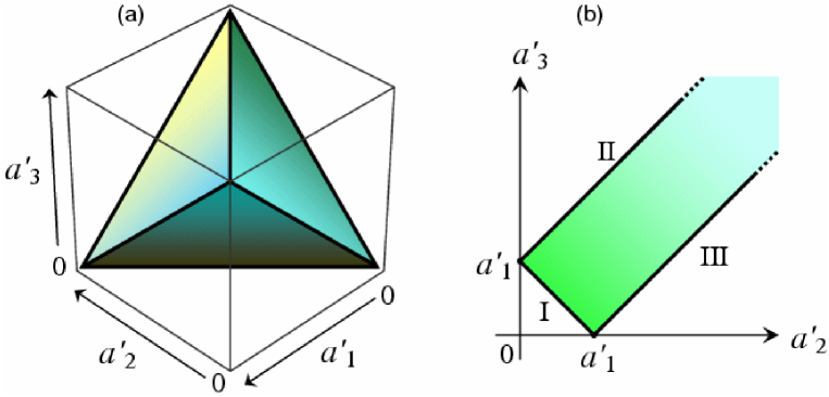
Figure 1: (color online) Range of the entropic quantities $a^{\prime}_{l}=\mu_{l}^{-1}-1$ for pure three-mode Gaussian states. The three parameters $a^{\prime}_{l}$, with $l=1,2,3$, have to vary inside the pyramid represented in plot (a) or, equivalently, for fixed values of one of them, say $a^{\prime}_{1}$, inside the shaded slice represented in plot (b), in order to determine the CM of a physical state, Eq. (42). The expression of the boundary surfaces/curves come from the saturation of the triangular inequality (40) for all possible mode permutations. In particular, for the projected two-dimensional plot (b), the equations of the three boundaries are: I. $a^{\prime}_{3}=a^{\prime}_{1}-a^{\prime}_{2}$; II. $a^{\prime}_{3}=a^{\prime}_{1}+a^{\prime}_{2}$; III. $a^{\prime}_{3}=a^{\prime}_{2}-a^{\prime}_{1}$.

Notice that conditions (35) and (37), although derived by assuming a specific bipartition of the three modes, are independent on the choice of the modes that enter in the considered bipartition, because they are invariant under all possible permutations of the modes. Defining the parameters

$$a^{\prime}_{l}\equiv a_{l}-1\;,$$ (38)

the Heisenberg uncertainty principle for single-mode states reduces to

$$a^{\prime}_{l}\geq 0\;\;\;\;\;\forall l=1,2,3\;.$$ (39)

This fact allows to greatly simplify the two previous conditions, which can be combined into the following triangular inequality

$$|a^{\prime}_{i}-a^{\prime}_{j}|\,\leq\,a^{\prime}_{k}\,\leq\,a^{\prime}_{i}+a^{\prime}_{j}\;.$$ (40)

Inequality (40) is a condition invariant under all possible permutations of the mode indexes $\{i,j,k\}$, and, together with the positivity of each $a^{\prime}_{l}$, fully characterizes the local symplectic eigenvalues of the CM of three-mode pure Gaussian states. It therefore provides a complete characterization of the entanglement in such states. All standard forms of pure three-mode Gaussian states and in particular, remarkably, all the possible values of the logarithmic negativity between any pair of subsystems, can be determined by letting $a^{\prime}_{1}$, $a^{\prime}_{2}$ and $a^{\prime}_{3}$ vary in their range of allowed values, as summarized in Fig. 1.

Let us remark that Eq. (40) qualifies itself as an entropic inequality, as the quantities $\{a^{\prime}_{j}\}$ are closely related to the purities and to the von Neumann entropies of the single-mode reduced states. In particular the von Neumann entropies $S_{Vj}$ of the reduced states are given by $S_{Vj}=f(a^{\prime}_{j}+1)=f(a_{j})$, where the increasing convex entropic function $f(x)$ has been defined in Eq. (8). Now, Inequality (40) is strikingly analogous to the well known triangle (Araki-Lieb) and subadditivity inequalities for the von Neumann entropy (holding for general systems, see, e.g., chuaniels ), which in our case read

$$|f(a_{i})-f(a_{j})|\leq f(a_{k})\leq f(a_{i})+f(a_{j})\;.$$ (41)

However, as the different convexity properties of the functions involved suggest, Inequalities (40) and (41) are not equivalent. Actually, as can be shown by exploiting the properties of the function $f(x)$, the Inequalities (40) imply the Inequalities (41) for both the leftmost and the rightmost parts. On the other hand, there exist values of the local symplectic eigenvalues $\{a_{j}\}$ for which Inequalities (41) are satisfied but (40) are violated. Therefore, the condition imposed by Eq. (40) is stronger than the generally holding inequalities for the von Neumann entropy applied to pure states.

Let us recall that the form of the CM of any Gaussian state can be simplified through local (unitary) symplectic operations (that therefore do not affect the entanglement or mixedness properties of the state) belonging to $Sp_{2,\mathbbm{R}}^{\oplus n}$. Such reductions of the CMs are called “standard forms”. For the sake of clarity, let us write the explicit standard form CM of a generic pure three-mode Gaussian state:

$$\boldsymbol{\sigma}^{p}_{sf}=\left(\begin{array}[]{cccccc}a_{1}&0&e_{12}^{+}&0&e_{13}^{+}&0\\ 0&a_{1}&0&e_{12}^{-}&0&e_{13}^{-}\\ e_{12}^{+}&0&a_{2}&0&e_{23}^{+}&0\\ 0&e_{12}^{-}&0&a_{2}&0&e_{23}^{-}\\ e_{13}^{+}&0&e_{23}^{+}&0&a_{3}&0\\ 0&e_{13}^{-}&0&e_{23}^{-}&0&a_{3}\end{array}\right)\;,$$ (42)

with

$$e_{ij}^{\pm}\equiv\frac{\sqrt{\left[\left(a_{i}-a_{j}\right)^{2}-\left(a_{k}-1\right)^{2}\right]\left[\left(a_{i}-a_{j}\right)^{2}-\left(a_{k}+1\right)^{2}\right]}\pm\sqrt{\left[\left(a_{i}+a_{j}\right)^{2}-\left(a_{k}-1\right)^{2}\right]\left[\left(a_{i}+a_{j}\right)^{2}-\left(a_{k}+1\right)^{2}\right]}}{4\sqrt{a_{i}a_{j}}}\,.$$ (43)

By direct comparison with Eq. (67) in Ref. extremal , it is immediate to verify that each two-mode reduced CM $\boldsymbol{\sigma}_{ij}$ denotes a standard form GLEMS with local purities $\mu_{i}=a_{i}^{-1}$ and $\mu_{j}=a_{j}^{-1}$, and global purity $\mu_{ij}\equiv\mu_{k}=a_{k}^{-1}$. From our study it then turns out that, regarding the classification of Sec. III kraus , pure three-mode Gaussian states may belong either to class 5, in which case they reduce to the global three-mode vacuum, or to class 2, reducing to the uncorrelated product of a single-mode vacuum and of a two-mode squeezed state, or to class 1 (fully inseparable state). No two-mode or three-mode biseparable pure three-mode Gaussian states are allowed.

Let us finally stress that, although useful in actual calculations, the use of CMs in standard form does not entail any loss of generality, because all the results derived in the present work do not depend on the choice of the specific form of the CMs, but only on invariant quantities, such as the global and local symplectic invariants.

III.2 Mixed states

The most general standard form $\boldsymbol{\sigma}_{sf}$ associated to the CM of any (generally mixed) three-mode Gaussian state can be written as

$$\boldsymbol{\sigma}_{sf}=\left(\begin{array}[]{cccccc}a_{1}&0&f_{1}&0&f_{3}&f_{5}\\ 0&a_{1}&0&f_{2}&0&f_{4}\\ f_{1}&0&a_{2}&0&f_{6}&f_{8}\\ 0&f_{2}&0&a_{2}&f_{9}&f_{7}\\ f_{3}&0&f_{6}&f_{9}&a_{3}&0\\ f_{5}&f_{4}&f_{8}&f_{7}&0&a_{3}\end{array}\right)\,,$$ (44)

where the 12 parameters $\{a_{j}\}$ (inverse of the local purities) and $\{f_{j}\}$ (the covariances describing correlations between the modes) are only constrained by the Heisenberg uncertainty relations Eq. (5). The possibility of this useful, general reduction can be easily proven along the same lines as the two-mode standard form reduction duan00 : by means of three local symplectic operations one can bring the three blocks $\boldsymbol{\sigma}_{1}$, $\boldsymbol{\sigma}_{2}$ and $\boldsymbol{\sigma}_{3}$ in Williamson form, thus making them insensitive to further local rotations (which are symplectic operations); exploiting such rotations on mode $1$ and $2$ one can then diagonalize the block $\boldsymbol{\varepsilon}_{12}$ as allowed by its singular value decomposition; finally, one local rotation on mode $3$ is left, by which one can cancel one entry of the block $\boldsymbol{\varepsilon}_{13}$. Indeed, the resulting number of free parameters could have been inferred by subtracting the number of parameters of an element of $Sp_{2,\mathbbm{R}}\oplus Sp_{2,\mathbbm{R}}\oplus Sp_{2,\mathbbm{R}}$ (which is $9$, as $Sp_{2,\mathbbm{R}}$ has $3$ independent generators) from the 21 entries of a generic $6\times 6$ symmetric matrix.

III.3 Symmetric states

Among generic Gaussian states, those endowed with some properties of symmetry under mode exchange play a special role for what concerns the structure of entanglement. In particular, in a three-mode CV system, bisymmetric states are Gaussian states invariant under the exchange of two given modes (say $2$ and $3$) unitarily ; adescaling . Their CM will be thus of the form

$$\boldsymbol{\sigma}_{bis}={\left(\begin{array}[]{ccc}\boldsymbol{\alpha}&\boldsymbol{\varepsilon}&\boldsymbol{\varepsilon}\\ \boldsymbol{\varepsilon}^{\sf T}&\boldsymbol{\beta}&\boldsymbol{\zeta}\\ \boldsymbol{\varepsilon}^{\sf T}&\boldsymbol{\zeta}^{\sf T}&\boldsymbol{\beta}\\ \end{array}\right)}\,.$$ (45)

Let mode $1$ be entangled with the block of modes $(23)$. It has been proven adescaling ; unitarily that for such bisymmetric states the application of a local unitary (symplectic in phase space) operation on the block $(23)$ concentrates the whole original multimode entanglement into the reduced state of a single pair of modes. Namely, in terms of the new modes $\{1,2^{\prime},3^{\prime}\}$, the CM is transformed in a two-mode entangled state of modes $1$ and $2^{\prime}$, tensor the uncorrelated single-mode state of mode $3^{\prime}$, so that the original multimode entanglement can be quantified resorting to the well established theory of bipartite entanglement in two-mode Gaussian states prl ; extremal ; eisplenio ; ciracfortshit ; francamentemeneinfischio .

The local symplectic transformation responsible for the unitary localization of the multimode entanglement is typically realized by a simple beam splitter, if the CM is in standard form, with the single-mode blocks in their Williamson diagonal form. More generally, it may be a combination of beam splitters, phase shifters and squeezers. This type of entanglement localization is unitary and reversible, and thus completely different from the usual localization or concentration procedures that are based on measurements, as in the case of the “localizable entanglement” previously introduced for spin systems localizprl ; localizpra ). To reconstruct the original state, it suffices to let the discarded mode $3^{\prime}$ interfere once more with mode $2^{\prime}$ through the reversed beam splitter (that is, by applying the inverse symplectic operation). We remark that the unitary localizability is a property that extends to all $1\times n$ Gaussian states adescaling , and to all $m\times n$ bisymmetric Gaussian states unitarily , enabling two parties (owing two respective blocks of multiple symmetric modes) to realize, by purely local controls, a perfect and reversible entanglement switch between two-mode and multimode quantum correlations.

Three-mode Gaussian states which are invariant under the exchange of any two modes are said to be fully symmetric. They are trivially bisymmetric with respect to any $1\times 2$ bipartition, meaning that each conceivable bipartite entanglement is locally equivalent to two-mode entanglement. In the Gaussian setting, these states are described by a CM adescaling ; unitarily

$$\boldsymbol{\sigma}_{s}={\left(\begin{array}[]{ccc}\boldsymbol{\alpha}&\boldsymbol{\varepsilon}&\boldsymbol{\varepsilon}\\ \boldsymbol{\varepsilon}^{\sf T}&\boldsymbol{\alpha}&\boldsymbol{\varepsilon}\\ \boldsymbol{\varepsilon}^{\sf T}&\boldsymbol{\varepsilon}^{\sf T}&\boldsymbol{\alpha}\\ \end{array}\right)}\,,$$ (46)

where the local mixedness $a\equiv\sqrt{{\rm Det}\,{\boldsymbol{\alpha}}}$ is the same for all the three modes. These states have been successfully produced in laboratory by quantum optical means 3mexp ; pfister , and exploited to implement quantum teleportation networks network ; naturusawa . Used as shared resources, they can be optimized with respect to local operations to realize CV teleportation with maximal nonclassical fidelity telepoppate , quantum secret sharing secret , controlled dense coding dense , and to solve CV Byzantine agreement sanpera . Moreover, the structure of tripartite entanglement in this kind of states presents peculiar sharing properties contangle , that are quite different from the properties of distributed entanglement among qubits and qudits sharing , as will be discussed in detail in Sec. V.3.

We finally mention that the unitary localizability of entanglement does not apply only to states with special symmetries. For instance, for all pure three-mode Gaussian states, the $1\times 2$ entanglement can be unitarily localized in any bipartition. This fact holds for generic pure Gaussian states of $1\times n$ bipartitions. botero ; unitarily ; adebook .

IV Genuine tripartite entanglement and entanglement sharing

In this section we approach in a systematic way the question of distributing quantum correlations among three parties globally prepared in a (pure or mixed) three-mode Gaussian state, and we deal with the related problem of quantifying genuine tripartite entanglement in such a state.

IV.1 Entanglement sharing

The key ingredient of our analysis is the so-called sharing or monogamy inequality, first introduced by Coffman, Kundu, and Wootters (CKW) CKW for systems of three qubits, and recently extended to systems of $n$ qubits by Osborne and Verstraete Osborne . The CKW monogamy inequality for a three-party system can be written as follows:

$$E^{i|(jk)}-E^{i|j}-E^{i|k}\geq 0\;,$$ (47)

where $i,\,j,\,k$ denote the three elementary parties (modes in a CV system), and $E$ refers to a proper measure of bipartite entanglement (in particular, nonnegative on inseparable states and monotonic under LOCC).

It is natural to expect that Ineq. (47) should hold for states of CV systems as well, despite the fact that they are defined on infinite-dimensional Hilbert spaces and can in principle achieve infinite entanglement, in particular the entanglement of distillation can become infinite in certain states of CV systems; these states can be defined and constructed rigorously using the techniques of field theory and statistical mechanics for the description of systems of infinitely many degrees of freedom Keyl . In fact, one can show that the linearity of quantum mechanics, through the so-called no-cloning theorem nocloning0 ; nocloning1 ; nocloning2 , prevents quantum correlations from being freely shareable, at striking variance with the behaviour of classical correlations sharing . This entails that quantum entanglement is “monogamous” monogam .

The crucial issue in contructing and proving the CV version of the CKW monogamy inequality is to find a proper measure of entanglement $E$, able to capture the trade-off between couplewise and tripartite correlations, quantitatively formalized by Ineq. (47). For qubit systems, such a measure is known as the tangle CKW . For Gaussian states of CV systems, this problem has been recently solved in Ref. contangle , where the CV analogue of the tangle has been defined and exploited to obtain a proof of the monogamy inequality (47) for all Gaussian states of three modes, and for all symmetric Gaussian states of systems with an arbitrary number of modes. Following the approach of Ref. contangle , we recall now the notation leading to the definition of the continous-variable tangle, and provide a detailed proof of the CKW monogamy inequality obeyed by all three-mode Gaussian states.

IV.2 The continuous-variable tangle

The continuous-variable tangle $E_{\tau}$ is formally defined as follows contangle . For a generic pure state $|\psi\rangle$ of a $(1+N)$–mode CV system, one has

$$E_{\tau}(\psi)\equiv\ln^{2}\|\tilde{\rho}\|_{1}\;,\qquad\rho=|\psi\rangle\!\langle\psi|\;.$$ (48)

This is a proper measure of bipartite entanglement, being a convex, increasing function of the logarithmic negativity $E_{\cal N}$, equivalent to the entropy of entanglement on pure states. For a pure Gaussian state $|\psi\rangle$ with CM $\boldsymbol{\sigma}^{p}$, it is easy to find that

$$E_{\tau}(\boldsymbol{\sigma}^{p})={\rm arcsinh}^{2}\left(\frac{\sqrt{1-\mu_{1}^{2}}}{\mu_{1}}\right)\;,$$ (49)

where $\mu_{1}=1/\sqrt{{\rm Det}\,\boldsymbol{\sigma}_{1}}$ is the local purity of the reduced state of mode $1$, described by a CM $\boldsymbol{\sigma}_{1}$ (we are considering a most general $1\times n$ bipartition). Def. (48) is naturally extended to generic mixed states $\rho$ of $(n+1)$–mode CV systems through the convex-roof formalism osbcroof . Namely,

$$E_{\tau}(\rho)\equiv\inf_{\{p_{i},\psi_{i}\}}\sum_{i}p_{i}E_{\tau}(\psi_{i})\,,$$ (50)

where the infimum is taken over all convex decompositions of $\rho$ in terms of pure states $\{|\psi_{i}\rangle\}$. If the index $i$ is continuous, the sum in Eq. (50) is replaced by an integral, and the probabilities $\{p_{i}\}$ by a probability distribution $\pi(\psi)$.

Next, it is important to recall that for two qubits the tangle can be equivalently defined as the convex roof of the squared negativity Lee , because the latter coincides with the concurrence for pure two-qubit states Wootters . Then, Eq. (50) states that the convex roof of the squared logarithmic negativity defines the proper continuous-variable tangle, or, in short, the contangle $E_{\tau}(\rho)$ contangle . One could have defined the contangle using the convex roof extension of the squared negativity as well. The two definitions are, in fact, equivalent to the aim of quantifying distributed entanglement, because the squared negativity is a convex function of the squared logarithmic negativity CKW ; sharing . The nice feature of using specifically the squared logarithmic negativity lies in the fact that from a computational point of view the logarithm accounts in a straightforard way for the infinite dimensionality of the underlying Hilbert sapce contangle . We will prove in the following that the contangle satisfies the CKW monogamy inequality for all three-mode Gaussian states. Viceversa, one can easily show that any continuous-variable tangle defined in terms of the (not squared) negativity or of the entanglement of formation fails to satisfy the CKW monogamy inequality in general contangle . This situation is to some extent reminiscent of the case of qubit systems, for which the CKW monogamy inequality holds using the tangle, defined as the convex roof of the squared concurrence CKW or of the squared negativity Lee , but fails if one chooses alternative definitions based on the convex roof of other equivalent measures of bipartite entanglement, such as the concurrence itself or the entanglement of formation CKW .

From now on, we restrict our attention to Gaussian states. Any multimode mixed Gaussian state with CM $\boldsymbol{\sigma}$, admits a decomposition in terms of pure Gaussian states only. The infimum of the average contangle, taken over all pure Gaussian state decompositions, defines the Gaussian contangle $G_{\tau}$

$$G_{\tau}(\boldsymbol{\sigma})\equiv\inf_{\{\pi(d\boldsymbol{\sigma}^{p}),\boldsymbol{\sigma}^{p}\}}\int\pi(d\boldsymbol{\sigma}^{p})E_{\tau}(\boldsymbol{\sigma}^{p})\;.$$ (51)

It follows from the convex roof construction that the Gaussian contangle $G_{\tau}(\boldsymbol{\sigma})$ is an upper bound to the true contangle $E_{\tau}(\boldsymbol{\sigma})$ (because the latter can be in principle minimized over a non-Gaussian decomposition):

$$E_{\tau}(\boldsymbol{\sigma})\,\leq\,G_{\tau}(\boldsymbol{\sigma})\;,$$ (52)

and it can be shown that $G_{\tau}(\boldsymbol{\sigma})$ is a bipartite entanglement monotone under Gaussian local operations and classical communications (GLOCC) geof ; ordering . The Gaussian contangle can be expressed in terms of CMs as

$$G_{\tau}(\boldsymbol{\sigma})=\inf_{\boldsymbol{\sigma}^{p}\leq\boldsymbol{\sigma}}E_{\tau}(\boldsymbol{\sigma}^{p})\;,$$ (53)

where the infimum runs over all pure Gaussian states with CM $\boldsymbol{\sigma}^{p}\leq\boldsymbol{\sigma}$. Let us remark that, if $\boldsymbol{\sigma}_{s}$ denotes a mixed symmetric ($1\times 1$)-mode Gaussian state, then the decomposition of $\boldsymbol{\sigma}_{s}$ in terms of an ensemble of pure Gaussian states is the optimal one eofprl , which means that the Gaussian contangle coincides with the true contangle. Moreover, the optimal pure-state CM $\boldsymbol{\sigma}_{s}^{p}$ minimizing $G_{\tau}(\boldsymbol{\sigma}_{s})$ in Eq. (53) is characterized by having $\tilde{\nu}_{-}(\tilde{\boldsymbol{\sigma}}^{p}_{s})=\tilde{\nu}_{-}(\tilde{\boldsymbol{\sigma}_{s}})$ eofprl ; geof . The fact that the smallest symplectic eigenvalue is the same for both partially transposed CMs entails for symmetric two-mode Gaussian states that

$$E_{\tau}(\boldsymbol{\sigma}_{s})=G_{\tau}(\boldsymbol{\sigma}_{s})=[\max\{0,-\ln\tilde{\nu}_{-}(\boldsymbol{\sigma}_{s})\}]^{2}\;.$$ (54)

Finally, of course $E_{\tau}=G_{\tau}$ as well in all pure Gaussian states of $1\times n$ bipartitions.

IV.3 Monogamy inequality for all three-mode Gaussian states

We now provide the detailed proof, first derived, among other results, in Ref. contangle , that all three-mode Gaussian states satisfy the CKW monogamy inequality (47), using the (Gaussian) contangle to quantify bipartite entanglement. The intermediate steps of the proof will be then useful for the subsequent computation of the residual genuine tripartite entanglement, as we will show in Sec. IV.4.

We start by considering pure three-mode Gaussian states, whose standard form CM $\boldsymbol{\sigma}^{p}$ is given by Eq. (42). As discussed in Sec. III.1, all the properties of entanglement in pure three-mode Gaussian states are completely determined by the three local purities. Reminding that the mixednesses $a_{l}\equiv 1/\mu_{l}$ have to vary constrained by the triangle inequality (40), in order for $\boldsymbol{\sigma}^{p}$ to represent a physical state, one has

$$|a_{j}-a_{k}|+1\leq a_{i}\leq a_{j}+a_{k}-1\;.$$ (55)

For ease of notation let us rename the mode indices so that $\{i,j,k\}\equiv\{1,2,3\}$. Without any loss of generality, we can assume $a_{1}>1$. In fact, if $a_{1}=1$ the first mode is not correlated with the other two and all the terms in Ineq. (47) are trivially zero. Moreover, we can restrict the discussion to the case of both the reduced two-mode states $\boldsymbol{\sigma}_{12}$ and $\boldsymbol{\sigma}_{13}$ being entangled. In fact, if e.g. $\boldsymbol{\sigma}_{13}$ denotes a separable state, then $E_{\tau}^{1|2}\leq E_{\tau}^{1|(23)}$ because tracing out mode $3$ is a LOCC, and thus the sharing inequality is automatically satisfied. We will now prove Ineq. (47) in general by using the Gaussian contangle, as this will immediately imply the inequality for the true contangle as well. In fact, $G_{\tau}^{1|(23)}(\boldsymbol{\sigma}^{p})=E_{\tau}^{1|(23)}(\boldsymbol{\sigma}^{p})$, but $G_{\tau}^{1|l}(\boldsymbol{\sigma})\geq E_{\tau}^{1|l}(\boldsymbol{\sigma}),\;l=2,3$.

Let us proceed by keeping $a_{1}$ fixed. From Eq. (49), it follows that the entanglement between mode $1$ and the remaining modes, $E_{\tau}^{1|(23)}={\rm arcsinh}^{2}\sqrt{a_{1}^{2}-1}$, is constant. We must now prove that the maximum value of the sum of the $1|2$ and $1|3$ bipartite entanglements can never exceed $E_{\tau}^{1|(23)}$, at fixed local mixedness $a_{1}$. Namely,

$$\max_{s,d}Q\,\leq\,{\rm arcsinh}^{2}\sqrt{a^{2}-1}\;,$$ (56)

where $a\equiv a_{1}$ (from now on we drop the subscript “1”), and we have defined

$$Q\,\equiv\,G_{\tau}^{1|2}(\boldsymbol{\sigma}^{p})+G_{\tau}^{1|3}(\boldsymbol{\sigma}^{p})\;.$$ (57)

The maximum in Eq. (56) is taken with respect to the “center of mass” and “relative” variables $s$ and $d$ that replace the local mixednesses $a_{2}$ and $a_{3}$ according to

$$s = \frac{a_{2}+a_{3}}{2}\;,$$ (58)

$$d = \frac{a_{2}-a_{3}}{2}\;.$$ (59)

The two parameters $s$ and $d$ are constrained to vary in the region

$$s\,\geq\,\frac{a+1}{2}\;,\;\;\qquad\left|d\right|\,\leq\,\frac{a^{2}-1}{4s}\;.$$ (60)

Ineq. (60) combines the triangle inequality (55) with the condition of inseparability for the states of the reduced bipartitions $(1|2)$ and $(1|3)$ ordering .

We recall now, as stated in Sec. III.1, that each $\boldsymbol{\sigma}_{1l}$, $l=2,3$, is a state of partial minimum uncertainty (GLEMS extremal ). For this class of states the Gaussian measures of entanglement, including $G_{\tau}$, can be computed explicitely ordering , yielding

$$Q={\rm arcsinh}^{2}\Big{[}\sqrt{m^{2}(a,s,d)-1}\Big{]}+{\rm arcsinh}^{2}\Big{[}\sqrt{m^{2}(a,s,-d)-1}\Big{]}\;,$$ (61)

where $m=m_{-}$ if $D\leq 0$, and $m=m_{+}$ otherwise (one has $m_{+}=m_{-}$ for $D=0$). Here:

$$m_{-} = \frac{|k_{-}|}{(s-d)^{2}-1}\;,$$

$$m_{+} = \frac{\sqrt{2\,\left[2a^{2}(1+2s^{2}+2d^{2})-(4s^{2}-1)(4d^{2}-1)-a^{4}-\sqrt{\delta}\right]}}{4(s-d)}\;,$$

$$D = 2(s-d)-\sqrt{2\left[k_{-}^{2}+2k_{+}+|k_{-}|(k_{-}^{2}+8k_{+})^{1/2}\right]/k_{+}}\;,$$

$$k_{\pm} = a^{2}\pm(s+d)^{2}\;,$$ (62)

and the quantity

$$\delta=(a-2d-1)(a-2d+1)(a+2d-1)(a+2d+1)(a-2s-1)(a-2s+1)(a+2s-1)(a+2s+1)$$

is the same as in Eq. (35). Note (we omitted the explicit dependence for brevity) that each quantity in Eq. (IV.3) is a function of $(a,s,d)$. Therefore, to evaluate the second term in Eq. (61) each $d$ in Eq. (IV.3) must be replaced by $-d$.

Studying the derivative of $m_{\mp}$ with respect to $s$, it is analytically proven that, in the whole range of parameters $\{a,s,d\}$ defined by Ineq. (60), both $m_{-}$ and $m_{+}$ are monotonically decreasing functions of $s$. The quantity $Q$ is then maximized over $s$ for the limiting value

$$s\,=\,s^{\min}\,\equiv\,\frac{a+1}{2}\;.$$ (63)

This value of $s$ corresponds to three-mode pure Gaussian states in which the state of the reduced bipartition $2|3$ is always separable, as one should expect because the bipartite entanglement is maximally concentrated in the states of the $1|2$ and $1|3$ reduced bipartitions. With the position Eq. (63), the quantity $D$ defined in Eq. (IV.3) can be easily shown to be always negative. Therefore, for both reduced CMs $\boldsymbol{\sigma}_{12}$ and $\boldsymbol{\sigma}_{13}$, the Gaussian contangle is defined in terms of $m_{-}$. The latter, in turn, acquires the simple form

$$m_{-}(a,s^{\min},d)\,=\,\frac{1+3a+2d}{3+a-2d}\;.$$ (64)

Consequently, the quantity $Q$ turns out to be an even and convex function of $d$, and this fact entails that it is globally maximized at the boundary

$$|d|\,=\,d^{\max}\,\equiv\,\frac{a-1}{2}\;.$$ (65)

We finally have that

$$Q^{\max} \equiv Q\left[a,s=s^{\min},d=\pm d^{\max}\right]$$ (66)

$$= {\rm arcsinh}^{2}\sqrt{a^{2}-1}\;,$$

which implies that in this case the sharing inequality (47) is exactly saturated and the genuine tripartite entanglement is consequently zero. In fact this case yields states with $a_{2}=a_{1}$ and $a_{3}=1$ (if $d=d^{\max}$), or $a_{3}=a_{1}$ and $a_{2}=1$ (if $d=-d^{\max}$), i.e. tensor products of a two-mode squeezed state and a single-mode uncorrelated vacuum. Being $Q^{\max}$ from Eq. (66) the global maximum of $Q$, Ineq. (56) holds true and the monogamy inequality (47) is thus proven for any pure three-mode Gaussian state, choosing either the Gaussian contangle $G_{\tau}$ or the true contangle $E_{\tau}$ as measures of bipartite entanglement contangle .

The proof immediately extends to all mixed three-mode Gaussian states $\boldsymbol{\sigma}$, but only if the bipartite entanglement is measured by $G_{\tau}(\boldsymbol{\sigma})$ Footnote . Let $\{\pi(d\boldsymbol{\sigma}^{p}_{m}),\boldsymbol{\sigma}^{p}_{m}\}$ be the ensemble of pure Gaussian states minimizing the Gaussian convex roof in Eq. (51); then, we have

$$G_{\tau}^{i|(jk)}(\boldsymbol{\sigma}) = \int\pi(d\boldsymbol{\sigma}^{p}_{m})G_{\tau}^{i|(jk)}(\boldsymbol{\sigma}^{p}_{m})$$

$$\geq \int\pi(d\boldsymbol{\sigma}^{p}_{m})[G_{\tau}^{i|j}(\boldsymbol{\sigma}^{p}_{m})+G_{\tau}^{i|k}(\boldsymbol{\sigma}^{p}_{m})]$$

$$\geq G_{\tau}^{i|j}(\boldsymbol{\sigma})+G_{\tau}^{i|k}(\boldsymbol{\sigma})\;,$$

where we exploited the fact that the Gaussian contangle is convex by construction. This concludes the proof of the CKW monogamy inequality (47) for all three-mode Gaussian states.

We close this subsection by discussing whether the CKW monogamy inequality can be generalized to all Gaussian states of systems with an arbitrary number $n+1$ of modes. Namely, we want to prove that

$$E^{i|(j_{1},\ldots,j_{n})}-\sum_{l=1}^{n}E^{i|j_{l}}\geq 0\;.$$ (68)

Establishing this result in general is a highly nontrivial task, but it can be readily proven for all symmetric multimode Gaussian states contangle . In a fully symmetric $n+1$-mode Gaussian state all the local purities are degenerate and reduce to a single parameter $a_{loc}$:

$$a_{i}\,=\,a_{j_{1}}\,=\,a_{j_{2}}\,=\,\dots\,=\,a_{j_{n}}\,\equiv\,a_{loc}\;.$$ (69)

As in the three-mode case, due to the convexity of $G_{\tau}$, it will suffice to prove Eq. (68) for pure states, for which the Gaussian contangle coincides with the true contangle in every bipartition. For any $n$ and for $a_{loc}>1$ (for $a_{loc}=1$ we have a product state), one has that

$$E_{\tau}^{i|(j_{1},\ldots,j_{n})}=\ln^{2}(a_{loc}-\sqrt{a_{loc}^{2}-1})$$ (70)

is independent of $n$, while the total two–mode contangle

$$nE_{\tau}^{i|j_{l}} = \frac{n}{4}\ln^{2}\bigg{\{}\Big{[}a_{loc}^{2}(n+1)-1$$

$$- \sqrt{(a_{loc}^{2}-1)(a_{loc}^{2}(n+1)^{2}-(n-1)^{2})}\;\;\Big{]}/n\bigg{\}}$$

is a monotonically decreasing function of the integer $n$ at fixed $a_{loc}$. Because the sharing inequality trivially holds for $n=1$, it is inductively proven for any $n$. This result, together with extensive numerical evidence obtained for randomly generated non-symmetric $4$–mode Gaussian states contangle , strongly supports the conjecture that the CKW monogamy inequality holds true for all multimode Gaussian state, using the (Gaussian) contangle as a measure of bipartite entanglement. However, at present, a fully analytical proof of this conjecture is still lacking.

IV.4 Residual contangle, genuine tripartite entanglement, and monotonicity

The sharing constraint leads naturally to the definition of the residual contangle as a quantifier of genuine tripartite entanglement (arravogliament) in three-mode Gaussian states, much in the same way as in systems of three qubits CKW . However, at variance with the three-qubit case, here the residual contangle is partition-dependent according to the choice of the reference mode, with the exception of the fully symmetric states. A bona fide quantification of tripartite entanglement is then provided by the minimum residual contangle contangle

$$E_{\tau}^{i|j|k}\equiv\min_{(i,j,k)}\left[E_{\tau}^{i|(jk)}-E_{\tau}^{i|j}-E_{\tau}^{i|k}\right]\;,$$ (72)

where the symbol $(i,j,k)$ denotes all the permutations of the three mode indexes. This definition ensures that $E_{\tau}^{i|j|k}$ is invariant under all permutations of the modes and is thus a genuine three-way property of any three-mode Gaussian state. We can adopt an analogous definition for the minimum residual Gaussian contangle $G_{\tau}^{res}$ (see Fig. 2 for a pictorial representation):

$$G_{\tau}^{res}\equiv G_{\tau}^{i|j|k}\equiv\min_{(i,j,k)}\left[G_{\tau}^{i|(jk)}-G_{\tau}^{i|j}-G_{\tau}^{i|k}\right]\;.$$ (73)

One can verify that

$$(G_{\tau}^{i|(jk)}\,-\,G_{\tau}^{i|k})\,-\,(G_{\tau}^{j|(ik)}\,-\,G_{\tau}^{j|k})\,\geq\,0$$ (74)

if and only if $a_{i}\geq a_{j}$, and therefore the absolute minimum in Eq. (72) is attained by the decomposition realized with respect to the reference mode $l$ of smallest local mixedness $a_{l}$, i.e. for the single-mode reduced state with CM of smallest determinant.

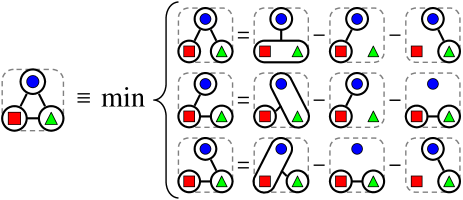
Figure 2: (color online) Pictorial representation of Eq. (73), defining the residual Gaussian contangle $G_{\tau}^{res}$ of generic (nonsymmetric) three-mode Gaussian states. $G_{\tau}^{res}$ quantifies the genuine tripartite entanglement shared among mode $1$ ($\color[rgb]{0,0,1}{\mathchoice{{\tf@size pt{}}}{{\tf@size pt{}}}{{\sf@size pt{}}}{{\ssf@size pt{}}}}$), mode $2$ ($\color[rgb]{1,0,0}{\blacksquare}$), and mode $3$ ($\color[rgb]{0,1,0}{\blacktriangle}$). The optimal decomposition that realizes the minimum in Eq. (73) is always the one for which the CM of the reduced state of the reference mode has the smallest determinant.

The residual (Gaussian) contangle must be nonincreasing under (Gaussian) LOCC in order to be a proper measure of tripartite entanglement. The monotonicity of the residual tangle was proven for three-qubit pure states in Ref. wstates . In the CV setting, it has been shown in Ref. contangle that for pure three-mode Gaussian states the residual Gaussian contangle Eq. (73) is an entanglement monotone under tripartite GLOCC, and that it is nonincreasing even under probabilistic operations, which is a stronger property than being only monotone on average. Therefore the Gaussian contangle $G_{\tau}^{res}$ defines (to the best of our knowledge) the first measure, proper and computable, of genuine multipartite (specifically, tripartite) entanglement in Gaussian states of CV systems. It is worth noting that the minimum in Eq. (73), that at first sight might appear a redundant requirement, is physically meaningful and mathematically necessary. In fact, if one chooses to fix a reference partition, or to take e.g. the maximum (and not the minimum) over all possible mode permutations in Eq. (73), the resulting “measure” is not monotone under GLOCC and thus is definitely not a measure of tripartite entanglement.

We now work out in detail an explicit application, by describing the complete procedure to determine the genuine tripartite entanglement in a pure three-mode Gaussian state $\boldsymbol{\sigma}^{p}$.

(i) Determine the local purities.

The state is globally pure (${\rm Det}\,\boldsymbol{\sigma}^{p}=1$); therefore, the only quantities needed for the computation of the tripartite entanglement are the three local mixednesses $a_{l}$, defined by Eq. (28), of the single-mode reduced states $\boldsymbol{\sigma}_{l},\,l=1,2,3$ (see Eq. (11)). Notice that the global CM $\boldsymbol{\sigma}^{p}$ needs not to be in the standard form (42), as the single-mode determinants are local symplectic invariants serafozzi . From an experimental point of view, the parameters $a_{l}$ can be extracted from the CM using the homodyne tomographic reconstruction of the state homotomo ; or they can be directly measured with the aid of single photon detectors fiuracerf ; wenger .

(ii) Find the minimum.

From Eq. (74), the minimum in the definition (73) of the residual Gaussian contangle $G_{\tau}^{res}$ is attained in the partition where the bipartite entanglements are decomposed choosing as reference mode $l$ the one in the single-mode reduced state of smallest local mixedness $a_{l}\equiv a_{min}$.

(iii) Check range and compute.

Given the mode with smallest local mixedness $a_{min}$ (say, for instance, mode $1$) and the parameters $s$ and $d$ defined in Eqs. (58,59), if $a_{min}=1$ then mode $1$ is uncorrelated from the others: $G_{\tau}^{res}=0$. If, instead, $a_{min}>1$ then

$$G_{\tau}^{res}(\boldsymbol{\sigma}^{p})={\rm arcsinh}^{2}\!\Big{[}\sqrt{a_{min}^{2}-1}\Big{]}-Q(a_{min},s,d)\;,$$ (75)

with $Q\equiv G_{\tau}^{1|2}+G_{\tau}^{1|3}$ defined by Eqs. (61,IV.3). Note that if $d<-(a_{min}^{2}-1)/4s$ then $G_{\tau}^{1|2}=0$. Instead, if $d>(a_{min}^{2}-1)/4s$ then $G_{\tau}^{1|3}=0$. Otherwise, all terms in $G_{\tau}^{res}$ Eq. (73) are nonvanishing.

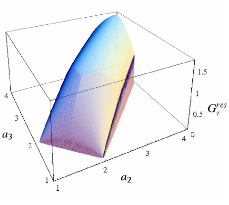
Figure 3: (color online) Three-dimensional plot of the residual Gaussian contangle $G_{\tau}^{res}(\boldsymbol{\sigma}^{p})$ in pure three-mode Gaussian states $\boldsymbol{\sigma}^{p}$, determined by the three local mixedness $a_{l}$, $l=1,2,3$. One of the local mixedness is kept fixed ($a_{1}=2$). The remaining ones vary constrained by the triangle inequality (55), as depicted in Fig. 1(b). The explicit expression of $G_{\tau}^{res}$ is given by Eq. (27). See text for further details.

The residual Gaussian contangle Eq. (73) in generic pure three-mode Gaussian states is plotted in Fig. 3 as a function of $a_{2}$ and $a_{3}$, at constant $a_{1}=2$. For fixed $a_{1}$, it is interesting to notice that $G_{\tau}^{res}$ is maximal for $a_{2}=a_{3}$, i.e. for bisymmetric states. Notice also how the residual Gaussian contangle of these bisymmetric pure states has a cusp for $a_{1}=a_{2}=a_{3}$. In fact, from Eq. (74), for $a_{2}=a_{3}<a_{1}$ the minimum in Eq. (73) is attained decomposing with respect to one of the two modes $2$ or $3$ (the result is the same by symmetry), while for $a_{2}=a_{3}>a_{1}$ mode $1$ becomes the reference mode.

For generic mixed three-mode Gaussian states, a quite cumbersome analytical expression for the $1|2$ and $1|3$ Gaussian contangles may be written geof ; ordering , involving the roots of a fourth order polynomial, but the optimization appearing in the computation of the $1|(23)$ bipartite Gaussian contangle (see Eq. (53)) has to be solved only numerically. However, exploiting techniques like the unitary localization unitarily described in Sec. III.3, and results like that of Eq. (54), closed expressions for the residual Gaussian contangle can be found as well in relevant classes of mixed three-mode Gaussian states endowed with some symmetry constraints. Interesting examples of these states and the investigation of their physical properties will be discussed in Sec. V.

As an additional remark, let us recall that, although the entanglement of Gaussian states is always distillable with respect to $1\times N$ bipartitions werwolf , they can exhibit bound entanglement in $1\times 1\times 1$ tripartitions kraus . In this case, the residual contangle cannot detect tripartite PPT entangled states. For example, the residual contangle in three-mode biseparable Gaussian states (class $4$ of Ref. kraus ) is always zero, because those bound entangled states are separable with respect to all $(1\times 2)$-mode bipartitions. In this sense we can correctly regard the residual contangle as an estimator of distillable tripartite entanglement in fully inseparable three-mode Gaussian states. However, we remind that this entanglement can be distilled only resorting to non-Gaussian LOCC browne , since distilling Gaussian states with Gaussian operations is impossible nogo1 ; nogo2 ; nogo3 .

V Sharing structure of tripartite entanglement

We are now in the position to analyze the sharing structure of CV entanglement in three-mode Gaussian states by taking the residual Gaussian contangle as a measure of tripartite entanglement, in analogy with the study done for three qubits wstates using the residual tangle CKW .

The first task we face is that of identifying the three-mode analogues of the two inequivalent classes of fully inseparable three-qubit states, the GHZ state ghzs

$$|\psi_{\rm GHZ}\rangle\,=\,\frac{1}{\sqrt{2}}\left(|000\rangle+|111\rangle\right)\;,$$ (76)

and the $W$ state wstates

$$|\psi_{W}\rangle\,=\,\frac{1}{\sqrt{3}}\left(|001\rangle+|010\rangle+|100\rangle\right)\;.$$ (77)

These states are both pure and fully symmetric, i.e. invariant under the exchange of any two qubits. On the one hand, the GHZ state possesses maximal tripartite entanglement, quantified by the residual tangle CKW ; wstates , with zero couplewise entanglement in any reduced state of two qubits reductions. Therefore its entanglement is very fragile against the loss of one or more subsystems. On the other hand, the $W$ state contains the maximal two-party entanglement in any reduced state of two qubits wstates and is thus maximally robust against decoherence, while its tripartite residual tangle vanishes.

V.1 CV GHZ/$W$ states

To define the CV counterparts of the three-qubit states $|\psi_{\rm GHZ}\rangle$ and $|\psi_{W}\rangle$, one must start from the fully symmetric three-mode CM $\boldsymbol{\sigma}_{s}$ of Eq. (46). Surprisingly enough, in symmetric three-mode Gaussian states, if one aims at maximizing, at given single-mode mixedness $a_{loc}\equiv a$, either the bipartite entanglement $G_{\tau}^{i|j}$ in any two-mode reduced state (i.e. aiming at the CV $W$-like state), or the genuine tripartite entanglement $G_{\tau}^{res}$ (i.e. aiming at the CV GHZ-like state), one finds the same, unique family of pure symmetric three-mode squeezed states $\boldsymbol{\sigma}^{p}_{s}$. These states, previously known as CV “GHZ-type” states network ; bravchap ; vanlokfuru , can be indeed defined for generic $n$-mode systems. They constitute an ideal test-ground for the study of the scaling of multimode CV entanglement with the number of modes. This analysis can be carried out via nested applications of the procedure of unitary localization adescaling ; unitarily , reviewed in Sec. III.3. For systems of three modes, they are described by a CM $\boldsymbol{\sigma}_{s}^{p}$ of the form Eq. (46), with $\boldsymbol{\alpha}=a\mathbbm{1}_{2}$, $\boldsymbol{\varepsilon}={\rm diag}\{e^{+},\,e^{-}\}$ and adescaling

$$e^{\pm}=\frac{a^{2}-1\pm\sqrt{\left(a^{2}-1\right)\left(9a^{2}-1\right)}}{4a}\;,$$ (78)

ensuring the global purity of the state. For self-explaining reasons, we choose to name these states “CV GHZ/$W$ states” contangle , and denote their CM by $\boldsymbol{\sigma}_{s}^{GHZ/W}$. In the limit of infinite squeezing ($a\rightarrow\infty$), the CV GHZ/$W$ state approaches the proper (unnormalizable) continuous-variable GHZ state $\int dx|x,x,x\rangle$, a simultaneous eigenstate of total momentum $\hat{p}_{1}+\hat{p}_{2}+\hat{p}_{3}$ and of all relative positions $\hat{x}_{i}-\hat{x}_{j}$ ($i,j=1,2,3$), with zero eigenvalues cvghz .

The residual Gaussian contangle of GHZ/$W$ states of finite squeezing takes the simple form contangle

$$\begin{split}G_{\tau}^{res}(\boldsymbol{\sigma}_{s}^{GHZ/W})&={\rm arcsinh}^{2}\!\left[\sqrt{a^{2}-1}\right]\\ &-\frac{1}{2}\ln^{2}\!\left[\frac{3a^{2}-1-\sqrt{9a^{4}-10a^{2}+1}}{2}\right]\,.\end{split}$$ (79)

It is straightforward to see that $G_{\tau}^{res}(\boldsymbol{\sigma}_{s}^{p})$ is nonvanishing as soon as $a>1$. Therefore, the GHZ/$W$ states belong to the class of fully inseparable three-mode states kraus ; adescaling ; network ; vloock02 ; vanlokfuru . We finally recall that in a GHZ/$W$ state the residual Gaussian contangle $G_{\tau}^{res}$ Eq. (73) coincides with the true residual contangle $E_{\tau}^{res}$ Eq. (72). This property clearly holds because the Gaussian pure-state decomposition is the optimal one in every bipartition, due to the fact that the global three-mode state is pure and the reduced two-mode states are symmetric.

V.2 $T$ states

The peculiar nature of entanglement sharing in CV GHZ/$W$ states is further confirmed by the following observation. If one requires maximization of the $1\times 2$ bipartite Gaussian contangle $G_{\tau}^{i|(jk)}$ under the constraint of separability of all the reduced two-mode states, one finds a class of symmetric mixed states characterized by being three-mode Gaussian states of partial minimum uncertainty. They are in fact characterized by having their smallest symplectic eigenvalue equal to $1$, and represent thus the three-mode generalization of two-mode symmetric GLEMS prl ; extremal ; ordering .

We will name these states $T$ states, with $T$ standing for tripartite entanglement only. They are described by a CM $\boldsymbol{\sigma}_{s}^{T}$ of the form Eq. (46), with $\boldsymbol{\alpha}=a\mathbbm{1}_{2}$, $\boldsymbol{\varepsilon}={\rm diag}\{e^{+},\,e^{-}\}$ and

$$e^{+} = \frac{a^{2}-5+\sqrt{9a^{2}\left(a^{2}-2\right)+25}}{4a}\;,$$

$$e^{-} = \frac{5-9a^{2}+\sqrt{9a^{2}\left(a^{2}-2\right)+25}}{12a}\;.$$ (80)

The $T$ states, like the GHZ/$W$ states, are determined only by the local mixedness $a$, are fully separable for $a=1$, and fully inseparable for $a>1$. The residual Gaussian contangle Eq. (73) can be analytically computed for these mixed states as a function of $a$. First of all one notices that, due to the complete symmetry of the state, each mode can be chosen indifferently to be the reference one in Eq. (73). Being the $1\times 1$ entanglements all zero by construction, $G_{\tau}^{res}=G_{\tau}^{i|(jk)}$. The $1\times 2$ bipartite Gaussian contangle can be in turn obtained exploiting the unitary localization procedure (see Sec. III.3). Let us choose mode $1$ as the reference mode and combine modes $2$ and $3$ at a 50:50 beam splitter, a local unitary operation with respect to the bipartition $1|(23)$ that defines the transformed modes $2^{\prime}$ and $3^{\prime}$. The CM $\boldsymbol{\sigma}_{s}^{T^{\prime}}$ of the state of modes $1$, $2^{\prime}$, and $3^{\prime}$ is then written in the following block form:

$$\boldsymbol{\sigma}_{s}^{T^{\prime}}=\left(\begin{array}[]{ccc}\boldsymbol{\sigma}_{1}&\boldsymbol{\varepsilon}_{12^{\prime}}&{\bf 0}\\ \boldsymbol{\varepsilon}_{12^{\prime}}^{\sf T}&\boldsymbol{\sigma}_{2^{\prime}}&{\bf 0}\\ {\bf 0}&{\bf 0}&\boldsymbol{\sigma}_{3^{\prime}}\\ \end{array}\right)\;,$$ (81)

where mode $3^{\prime}$ is now disentangled from the others. Thus

$$G_{\tau}^{1|(23)}(\boldsymbol{\sigma}_{s}^{T})=G_{\tau}^{1|2^{\prime}}(\boldsymbol{\sigma}_{s}^{T^{\prime}})\;.$$ (82)

Moreover, the reduced CM $\boldsymbol{\sigma}_{12^{\prime}}$ of modes $1$ and $2^{\prime}$ defines a nonsymmetric GLEM prl ; extremal with

$${\rm Det}\,\boldsymbol{\sigma}_{1} = a^{2}\,,$$

$${\rm Det}\,\boldsymbol{\sigma}_{2} = \frac{1}{6}\left(3a^{2}+\sqrt{9\left(a^{2}-2\right)a^{2}+25}-1\right)\,,$$

$${\rm Det}\,\boldsymbol{\sigma}_{12^{\prime}} = \frac{1}{2}\left(3a^{2}-\sqrt{9\left(a^{2}-2\right)a^{2}+25}+3\right)\,,$$

and it has been shown that the Gaussian contangle is computable in two-mode GLEMS ordering . After some algebra, one finds the complete expression of $G_{\tau}^{res}$ for $T$ states:

$$G_{\tau}^{res}(\boldsymbol{\sigma}_{s}^{T}) = {\rm arcsinh}^{2}\Bigg{\{}\bigg{[}25R-9a^{4}+3Ra^{2}+6a^{2}-109$$ (83)

$$- \Big{(}81a^{8}-432a^{6}+954a^{4}-1704a^{2}+2125$$

$$- \left(3a^{2}-11\right)\left(3a^{2}-7\right)\left(3a^{2}+5\right)R\Big{)}^{\frac{1}{2}}\sqrt{2}\bigg{]}^{\frac{1}{2}}$$

$$\times \left[{18\left(3a^{2}-R+3\right)}\right]^{-\frac{1}{2}}\Bigg{\}}\;,$$

with $R\equiv\sqrt{9a^{2}(a^{2}-2)+25}$.

What is remarkable about $T$ states is that their tripartite Gaussian contangle Eq. (83) is strictly smaller than the one of the GHZ/$W$ states Eq. (79) for any fixed value of the local mixedness $a$, that is, for any fixed value of the only parameter (operationally related to the squeezing of each single mode) that completely determines the CMs of both families of states up to local unitary operations. This hyerardical behavior of the residual contangle in the two classes of states is illustrated in Fig. 4. Notice that this result cannot be an artifact caused by restricting to pure Gaussian decompositions only in the definition Eq. (73) of the residual Gaussian contangle. In fact, for $T$ states the relation $G_{\tau}^{res}(\boldsymbol{\sigma}_{s}^{T})\geq E_{\tau}^{res}(\boldsymbol{\sigma}_{s}^{T})$ holds due to the symmetry of the reduced two-mode states, and to the fact that the unitarily transformed state of modes $1$ and $2^{\prime}$ is mixed and nonsymmetric. The crucial consequences of this result for the structure of the entanglement trade-off in Gaussian states will be discussed further in the next subsection.

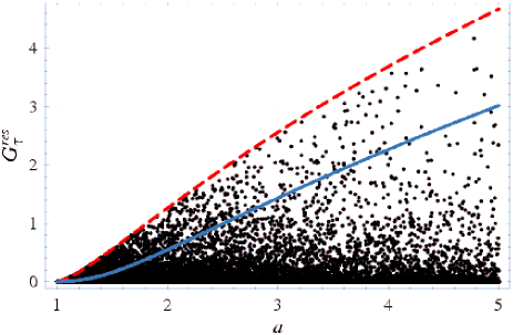
Figure 4: (color online) Plot, as a function of the single-mode mixedness $a$, of the tripartite residual Gaussian contangle $G_{\tau}^{res}$ Eq. (79) in the CV GHZ/$W$ states (dashed line); in the $T$ states Eq. (83) (solid line); and in 50000 randomly generated mixed symmetric three-mode Gaussian states of the form Eq. (46) (dots). The GHZ/$W$ states, that maximize any bipartite entanglement, also achieve maximal genuine tripartite quantum correlations, showing that CV entanglement distributes in a promiscuous way in symmetric Gaussian states. Notice also how all random mixed states have a nonnegative residual Gaussian contangle. This confirms the results presented in Ref. contangle , and discussed in detail and extended in Sec. IV.3, on the strict validity of the CKW monogamy inequality for CV entanglement in three-mode Gaussian states.

V.3 Promiscuous continuous-variable entanglement sharing

The above results, pictorially illustrated in Fig. 4, lead to the conclusion that in symmetric three-mode Gaussian states, when there is no bipartite entanglement in the two-mode reduced states (like in $T$ states) the genuine tripartite entanglement is not enhanced, but frustrated. More than that, if there are maximal quantum correlations in a three-party relation, like in GHZ/$W$ states, then the two-mode reduced states of any pair of modes are maximally entangled mixed states.

These findings, unveiling a major difference between discrete-variable (mainly qubits) and continuous-variable systems, establish the promiscuous nature of CV entanglement sharing in symmetric Gaussian states contangle ; sharing . Being associated with degrees of freedom with continuous spectra, states of CV systems need not saturate the CKW inequality to achieve maximum couplewise correlations. In fact, without violating the monogamy constraint Ineq. (47), pure symmetric three-mode Gaussian states are maximally three-way entangled and, at the same time, maximally robust against the loss of one of the modes. This preselects GHZ/$W$ states also as optimal candidates for carrying quantum information through a lossy channel, being, for their intrinsic entanglement structure, less sensitive to decoherence effects, as we will show in Sec. VI.

As an additional remark, let us mention that, quite naturally, not all three-mode Gaussian states (in particular nonsymmetric states) are expected to exhibit a promiscuous entanglement sharing. Further investigations to clarify the sharing structure of generic Gaussian states of CV systems, and the origin of the promiscuity, are currently under way 3mjpart1 . As an anticipation, we can mention that promiscuity tends to survive even in the presence of mixedness of the state, but is destroyed by the loss of complete symmetry. The powerful consequences of the entanglement properties of GHZ/$W$ states for experimental implementations of CV quantum-information protocols are currently under investigation 3mjpart2 .

VI Decoherence of three-mode states and decay of tripartite entanglement

Remarkably, Gaussian states allow for a straightforward, analytical treatment of decoherence, accounting for the most common situations encountered in the experimental practice (like fibre propagations or cavity decays) and even for more general, ‘exotic’ settings (like “squeezed” or common reservoirs) serafozzijob05 . This agreeable feature, together with the possibility – extensively exploited in this paper – of exactly computing several interesting benchmarks for such states, make Gaussian states a useful theoretical reference for investigating the effect of decoherence on the information and correlation content of quantum states. Let us mention that the dissipative evolution of three-mode states has been considered in Ref. paris05 , addressing SU(2,1) coherent states and focusing essentially on separability thresholds and telecloning efficiencies. In this section, we will explicitly show how the decoherence of three-mode Gaussian states may be exactly studied for any finite temperature, focusing on the evolution of the residual contangle as a measure of tripartite correlations. The results here obtained will be recovered in future work 3mjpart2 , and applied to the study of the effect of decoherence on multiparty protocols of CV quantum communication with the classes of states we are addressing, thus completing the present analysis by investigating its precise operational consequences. Concerning the general theory of open quantum dynamics, it is impossible here to give a detailed account of all the aspects of the standard theoretical frameworks. For an excellent critical review, focusing on the standard treatment of open quantum systems in relation to quantum entanglement see Ref. Benatti . In this ample review the authors discuss the importance of notions such as complete positivity, a physically motivated algebraic constraint on the quantum dynamics, in relation to quantum entanglement, and analyze the entanglement power of heat baths versus their decohering properties.

For continuous-variable systems, in the most customary and relevant instances the bath interacting with a set of $n$ modes can be modeled by $n$ independent continua of oscillators, coupled to the bath through a quadratic Hamiltonian $H_{int}$ in rotating wave approximation, reading

$$H_{int}=\sum_{i=1}^{n}\int v_{i}(\omega)[a_{i}^{{\dagger}}b_{i}(\omega)+a_{i}b_{i}^{{\dagger}}(\omega)]\,{\rm d}\omega\,,$$ (84)

where $b_{i}(\omega)$ stands for the annihilation operator of the $i$th continuum’s mode labeled by the frequency $\omega$, whereas $v_{i}(\omega)$ represents the coupling of such a mode to the mode $i$ of the system (assumed, for simplicity, to be real). The state of the bath is assumed to be stationary. Under the Born-Markov approximation bornmarkov , the Hamiltonian $H_{int}$ leads, upon partial tracing over the bath, to the following master equation for the $n$ modes of the system (in interaction picture) carmichael

$$\dot{\varrho}\;=\;\sum_{i=1}^{n}\frac{\gamma_{i}}{2}\Big{(}N_{i}\>L[a_{i}^{{\dagger}}]\varrho+(N_{i}+1)\>L[a_{i}]\varrho\Big{)}\,,$$ (85)

where the dot stands for time–derivative, the Lindblad superoperators are defined as $L[\hat{o}]\varrho\equiv 2\hat{o}\varrho\hat{o}^{{\dagger}}-\hat{o}^{{\dagger}}\hat{o}\varrho-\varrho\hat{o}^{{\dagger}}\hat{o}$, the couplings are $\gamma_{i}=2\pi v_{i}^{2}(\omega_{i})$, whereas the coefficients $N_{i}$ are defined in terms of the correlation functions $\langle b_{i}^{{\dagger}}(\omega_{i})b_{i}(\omega_{i})\rangle=N_{i}$, where averages are computed over the state of the bath and $\omega_{i}$ is the frequency of mode $i$. Notice that $N_{i}$ is the number of thermal photons present in the reservoir associated to mode $i$, related to the temperature $T_{i}$ of the reservoir by the Bose statistics at null chemical potential:

$$N_{i}=\frac{1}{{\exp}({\frac{\omega_{i}\hbar}{kT_{i}}})-1}\;.$$ (86)

In the derivation, we have also assumed $\langle b_{i}(\omega_{i})b_{i}(\omega_{i})\rangle=0$, holding for a bath at thermal equilibrium. We will henceforth refer to a “homogeneous” bath in the case $N_{i}=N$ and $\gamma_{i}=\gamma$ for all $i$.

Now, the master equation (85) admits a simple and physically transparent representation as a diffusion equation for the time-dependent characteristic function of the system $\chi(\xi,t)$ carmichael

$$\dot{\chi}(\xi,t)=-\sum_{i=1}^{n}\frac{\gamma_{i}}{2}\Bigg{[}(x_{i}\;p_{i}){\partial{x_{i}}\choose\partial{p_{i}}}+(x_{i}\;p_{i})\boldsymbol{\omega}^{\sf T}\boldsymbol{\sigma}_{i\infty}\boldsymbol{\omega}{x_{i}\choose p_{i}}\Bigg{]}\chi(\xi,t)\,,$$ (87)

where $\xi\equiv(x_{1},p_{1},\ldots,x_{n},p_{n})$ is a phase-space vector, $\boldsymbol{\sigma}_{i\infty}=\,{\rm diag}\,(2N_{i}+1,2N_{i}+1)$ and ${\boldsymbol{\omega}}$ is the $2\times 2$ symplectic form [defined in Eq. (1)]. The right hand side of the previous equation contains a deterministic drift term, which has the effect of damping the first moments to zero on a time scale of $\gamma/2$ and a diffusion term with diffusion matrix $\boldsymbol{\sigma}_{\infty}\equiv\oplus_{i=1}^{n}\boldsymbol{\sigma}_{i\infty}$. The essential point here is that Eq. (87) preserves the Gaussian character of the initial state, as can be straightforwardly checked for any initial CM $\boldsymbol{\sigma}_{0}$ by inserting the Gaussian characteristic function $\chi(\xi,t)$ [see Eq. (4)]

$$\chi(\xi,t)=\,{\rm e}^{-\frac{1}{2}\xi^{\sf T}\Omega^{\sf T}\boldsymbol{\sigma}(t)\Omega\xi+iX^{\sf T}\Gamma_{t}\Omega\xi}\;$$

(where $X$ are generic initial first moments, $\boldsymbol{\sigma}(t)\equiv\Gamma_{t}^{2}\boldsymbol{\sigma}_{0}+(\mathbbm{1}-\Gamma_{t}^{2})\boldsymbol{\sigma}_{\infty}$ and $\Gamma_{t}\equiv\oplus_{i}{\rm e}^{-\gamma_{i}t/2}\mathbbm{1}_{2}$) into the equation and verifying that it is indeed a solution. Notice that, for a homogeneous bath, the diagonal matrices $\Gamma_{t}$ and $\boldsymbol{\sigma}_{\infty}$ (providing a full characterisation of the bath) are both proportional to the identity. In order to keep track of the decay of correlations of Gaussian states, we are interested in the evolution of the initial CM $\boldsymbol{\sigma}_{0}$ under the action of the bath which, recalling our previous Gaussian solution, is just described by

$$\boldsymbol{\sigma}(t)=\Gamma_{t}^{2}\boldsymbol{\sigma}_{0}+(\mathbbm{1}-\Gamma_{t}^{2})\boldsymbol{\sigma}_{\infty}\;$$ (88)

This simple equation describes the dissipative evolution of the CM of any initial state under the action of a thermal environment and, at zero temperature, under the action of “pure losses” (recovered in the instance $N_{i}=0$ for $i=1,\ldots,n$). It yields a basic, significant example of ‘Gaussian channel’, i.e. of a map mapping Gaussian states into Gaussian states under generally non unitary evolutions. Exploiting Eq. (88) and our previous findings, we can now study the exact evolution of the tripartite entanglement of Gaussian states under the decoherent action of losses and thermal noise. For simplicity, we will mainly consider homogeneous baths.

As a first general remark let us notice that, in the case of a zero temperature bath ($N=0$), in which decoherence is entirely due to losses, the bipartite entanglement between any different partitions decays in time but persists for an infinite time. This is a general property of Gaussian entanglement serafozzijob05 under any many mode bipartition. The same fact is also true for the genuine tripartite entanglement, quantified by the residual contangle. If $N\neq 0$, a finite time does exist for which tripartite quantum correlations disappear. In general, the two-mode entanglement between any given mode and any other of the remaining two modes vanishes before than the three-mode bipartite entanglement between such a mode and the other two [not surprisingly, as the former quantity is, at the beginning, bounded by the latter because of the CKW monogamy inequality (47)].

The main issue addressed in this analysis has consisted in inspecting the robustness of different forms of genuine tripartite entanglement, previously introduced in the paper. Notice that an analogous question has been addressed in the qubit scenario, by comparing the action of decoherence on the residual tangle of the inequivalent sets of GHZ and $W$ states: $W$ states, which are by definition more robust under subsystem erasure, proved more robust under decoherence as well carvalho04 . In our instance, the symmetric GHZ/$W$ states constitute a promising candidate for the role of most robust Gaussian tripartite entangled states, as somehow expected. Evidence supporting this conjecture is shown in Fig. 5, where the evolution in different baths of the tripartite entanglement of GHZ/$W$ states is compared to that of symmetric $T$ states (at same initial entanglement). No fully symmetric states with tripartite entanglement more robust than GHZ/$W$ states were found by further numerical inspection. Quite remarkably, the promiscuous sharing of quantum correlations, proper to GHZ/W states, appears to better preserve genuine multipartite entanglement against the action of decoherence.

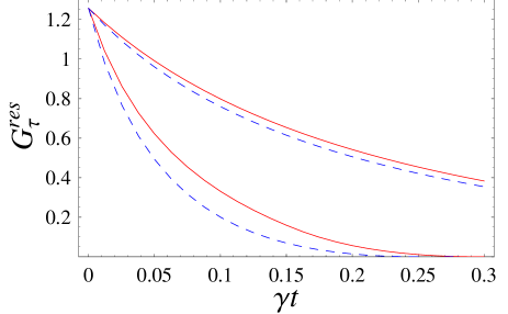
Figure 5: (color online) Evolution of the residual Gaussian contangle $G^{res}_{\tau}$ for GHZ/$W$ states with local mixedness $a=2$ (solid curves) and $T$ states with local mixedness $a=2.8014$ (dashed curves). Such states have equal initial residual contangle. The uppermost curves refer to a homogeneous bath with $N=0$ (pure losses), while the lowermost curves refer to a homogeneous bath with $N=1$. As apparent, thermal photons are responsible for the vanishing of entanglement at finite times.

Notice also that, for a homogeneous bath and for all fully symmetric and bisymmetric three-mode states, the decoherence of the global bipartite entanglement of the state is the same as that of the corresponding equivalent two-mode states (obtained through unitary localization). Indeed, for any bisymmetric state which can be localized by an orthogonal transformation (like a beam-splitter), the unitary localization and the action of the decoherent map of Eq. (88) commute, because $\boldsymbol{\sigma}_{\infty}\propto\mathbbm{1}$ is obviously preserved under orthogonal transformations (note that the bisymmetry of the state is maintained through the channel, due to the symmetry of the latter). In such cases, the decoherence of the bipartite entanglement of the original three-mode state (with genuine tripartite correlations) is exactly equivalent to that of the corresponding initial two-mode state obtained by unitary localization. This equivalence breaks down, even for GHZ/$W$ states which can be localized through an (orthogonal) beam-splitter transformation, for non homogeneous baths, i.e.  if the thermal photon numbers $N_{i}$ related to different modes are different [which is the case for different temperatures $T_{i}$ or for different frequencies $\omega_{i}$, according to Eq. (86)] or if the couplings $\gamma_{i}$ are different. In this instance let us remark that unitary localization could provide a way to cope with decoherence, limiting its hindering effect on entanglement. In fact, let us suppose that a given amount of genuine tripartite entanglement is stored in a symmetric (unitarily localizable) three-mode state and is meant to be exploited, at some (later) time, to implement tripartite protocols. During the period going from its creation to its actual use such an entanglement decays under the action of decoherence. Suppose the three modes involved in the process do not decay with the same rate (different $\gamma_{i}$) or under the same amount of thermal photons (different $N_{i}$), then the obvious, optimal way to shield tripartite entanglement is concentrating it, by unitary localization, in the two least decoherent modes. The entanglement can then be redistributed among the three modes by a reversal unitary operation, just before employing the state. Of course, the concentration and distribution of entanglement require a high degree of non local control on two of the three-modes, which would not always be allowed in realistic operating conditions.

The bipartite entanglement of GHZ/$W$ states (under $(1+2)$-mode bipartitions) decays slightly faster (in homogeneous baths with equal number of photons) than that of an initial pure two-mode squeezed state (also known as “twin-beam” state) with the same initial entanglement. In this respect, multimode entanglement is more fragile than two-mode, as the Hilbert space exposed to decoherence which contains it is larger. Notice that this claim does not refute the one of Ref. paris05 , where SU(2,1) coherent states were found to be as robust as corresponding two-mode states, but only for the same total number of thermal photons in the multimode channels.

VII Concluding remarks and outlook

Gaussian states distinctively stand out in the infinite variety of quantum states of continuous-variable systems, both for the analytic description they allow in terms of covariance matrices and symplectic operations, and for the high standards currently reached in their experimental production, manipulation and implementation for CV quantum information processing. Still, some recent results demonstrate that basically the current state of the art in the theoretical understanding and experimental control of CV entanglement is strongly pushing towards the boundaries of the “ideal” realm of Gaussian states and Gaussian operations. For instance, Gaussian entanglement cannot be distilled by Gaussian operations alone nogo1 ; nogo2 ; nogo3 , and moreover Gaussian states are “extremal”, in the sense that they are the least entangled among all states of CV systems with a given CM wolfext . On the other hand, however, some important pieces of knowledge in the theory of entanglement of Gaussian states are still lacking. The most important asymptotic measures of entanglement endowed with a physical meaning, the entanglement cost and the entanglement of distillation cannot be computed, and the entanglement of formation is computable only in the special case of two-mode, symmetric Gaussian states eofprl . Moreover, when moving to consider multipartite entanglement, many of the basic questions are still unanswered, much like in the case of multipartite entanglement in states of many qubits.

In this work we took a step ahead in the characterization of multipartite entanglement in Gaussian states. We focused on the prototypical structure of a CV system with more than two parties, that is a three-mode system prepared in a Gaussian state. We completed the elegant qualificative classification of separability in three-mode Gaussian states provided in Ref. kraus with an exhaustive, quantitative characterization of the various forms of quantum correlations that can arise among the three parties. We then exploited some recent results on entanglement sharing in multimode Gaussian states contangle that prove that CV entanglement in these states is indeed monogamous in the sense of the Coffman-Kundu-Wootters monogamy inequality CKW . We next defined a measure of genuine tripartite entanglement, the residual continuous-variable tangle, that turns out to be an entanglement monotone under tripartite Gaussian LOCC contangle .

We started our analysis by giving a complete characterization of pure and mixed three-mode Gaussian states, and deriving the standard forms of the covariance matrices that are similar to those known for two-mode states duan00 . In particular, a generic pure three-mode Gaussian states is completely specified, in standard form, by three parameters, which are the purities (determinants of the CMs) of the reduced states for each mode. We determined analytically the general expression of the genuine tripartite entanglement in pure three-mode Gaussian states, and studied its properties in comparison with the bipartite entanglement across different partitions. We investigated the sharing structure underlying the distribution of quantum correlations among three modes in arbitrary Gaussian states, much on the same lines as those followed in the case of states of three qubits wstates .

Remarkably, we found a completely unique feature, namely that that there exists a special class of states, the pure, symmetric, three-mode squeezed states, which simultaneously maximize the genuine tripartite entanglement and the bipartite entanglement in the reduced states of any pair of modes. This property, which has no counterpart in finite-dimensional systems, can be understood as the promiscuous sharing of CV entanglement. The states exhibiting this peculiar sharing structure, named CV “GHZ/$W$” states for self-explaining reasons, are automatically preselected as optimal carriers of quantum information over lossy channels, and we proved that they indeed are. In fact, we concluded our work with a detailed analysis of the effects of decoherence on three-mode Gaussian states and the decay of tripartite entanglement. This study yielded that the GHZ/$W$ states are the most robust three-party entangled Gaussian states against decoherence.

We believe that the collection of results presented here, although remarkable on its own, is however only the tip of an iceberg. Three-mode Gaussian states, the perfect test-ground for the understanding of some generic traits of multipartite entanglement in CV systems, need to be analyzed in a deeper future perspective. This primarily includes the characterization of those classes of tripartite entangled states with peculiar properties, with a particular care towards their state engineering in quantum optical settings. This analysis is currently under way 3mjpart1 . The (closely related) usefulness of such states for existing and maybe novel protocols of CV quantum communication, able to take advantage from the promiscuous sharing, is also being investigated 3mjpart2 .

From a broader theoretical standpoint, further research stemming from the present work should probably be directed along two main directions. The first one concerns proving a general monogamy inequality in all multimode states of CV systems, in analogy to what has been recently established for arbitrary states of multiqubit systems Osborne . Such a proof would then lead to a multimode generalization of the residual contangle. The second, long-term direction is the investigation of the qualitative and quantitative aspects of entanglement in generic non-Gaussian states of CV systems. In this context, singling out exotic states with enhanced promiscuous sharing of quantum correlations and with a monogamy of entanglement stretched to its limits, appears as an exciting perspective, and might open very promising perspectives for the manipulation, transfer, and control of quantum information with continuous variables.

- (1) M. A. Nielsen and I. L. Chuang, Quantum Information and Quantum Computation (Cambridge University Press, Cambridge 2000).
- (2) J. I. Cirac, in Fundamentals of Quantum Information, edited by D. Heiss (Springer-Verlag, Heidelberg-Berlin, 2002).
- (3) V. Coffman, J. Kundu, and W. K. Wootters, Phys. Rev. A 61, 052306 (2000).
- (4) T. J. Osborne and F. Verstraete, quant-ph/0502176.
- (5) Quantum Information Theory with Continuous Variables, edited by S. L. Braunstein and A. K. Pati (Kluwer Academic Publishers, Dordrecht, 2003).
- (6) Quantum Information with Continuous Variables of Atoms and Light, edited by N. J. Cerf, G. Leuchs, and E. S. Polzik (Imperial College Press, London, in press).
- (7) S. L. Braunstein and P. van Loock, Rev. Mod. Phys. 77, 513 (2005).
- (8) J. Eisert and M. B. Plenio, Int. J. Quant. Inf. 1, 479 (2003).
- (9) G. Adesso, A. Serafini, and F. Illuminati, Phys. Rev. Lett. 92, 087901 (2004).
- (10) G. Adesso, A. Serafini, and F. Illuminati, Phys. Rev. A 70, 022318 (2004).
- (11) G. Giedke, B. Kraus, M. Lewenstein, and J. I. Cirac, Phys. Rev. A 64, 052303 (2001).
- (12) G. Adesso and F. Illuminati, New J. Phys. 8, 15 (2006).
- (13) G. Adesso and F. Illuminati, quant-ph/0506213, Int. J. Quant. Inf. (in press).
- (14) J. Laurat, G. Keller, J. A. Oliveira-Huguenin, C. Fabre, T. Coudreau, A. Serafini, G. Adesso, and F. Illuminati, J. Opt. B: Quant. Semiclass. Optics 7, S577 (2005).
- (15) G. B. Folland, Harmonic analysis in phase space (Princeton University Press, Princeton, 1989).
- (16) Arvind, B. Dutta, N. Mukunda, and R. Simon, Pramana: J. Phys. 45, 471 (1995).
- (17) J. Williamson, Am. J. Math. 58, 141 (1936).
- (18) R. Simon, S. Chaturvedi, and V. Srinivasan, J. Math. Phys. 40, 3632 (1999).
- (19) A. Serafini, F. Illuminati, and S. De Siena, J. Phys. B: At. Mol. Opt. Phys. 37, L21 (2004).
- (20) A. Peres, Phys. Rev. Lett. 77, 1413 (1996).
- (21) M. Horodecki, P. Horodecki, and R. Horodecki, Phys. Lett. A 223, 1 (1996).
- (22) R. Simon, Phys. Rev. Lett. 84, 2726 (2000).
- (23) R. F. Werner and M. M. Wolf, Phys. Rev. Lett. 86, 3658 (2001).
- (24) A. Serafini, G. Adesso, and F. Illuminati, Phys. Rev. A 71, 032349 (2005).
- (25) G. Giedke, B. Kraus, M. Lewenstein, and J. I. Cirac, Phys. Rev. Lett. 64, 052313 (2001).
- (26) G. Vidal and R. F. Werner, Phys. Rev. A 65, 032314 (2002).
- (27) A. Serafini, Phys. Rev. Lett. 96, 110402 (2006).
- (28) K. Zyczkowski, P. Horodecki, A. Sanpera, and M. Lewenstein, Phys. Rev. A 58, 883 (1998).
- (29) J. Eisert, PhD Thesis (University of Potsdam, Potsdam, 2001).
- (30) K. Audenaert, M. B. Plenio, and J. Eisert, Phys. Rev. Lett. 90, 027901 (2003).
- (31) M. B. Plenio, Phys. Rev. Lett. 95, 090503 (2005).
- (32) C. H. Bennett, D. P. DiVincenzo, J. A. Smolin, and W. K. Wootters, Phys. Rev. A 54, 3824 (1996).
- (33) G. Giedke, M. M. Wolf, O. Krüger, R. F. Werner, and J. I. Cirac, Phys. Rev. Lett. 91, 107901 (2003).
- (34) P. M. Hayden, M. Horodecki, and B. M. Terhal, J. Phys. A: Math. Gen. 34, 6891 (2001).
- (35) G. Adesso and F. Illuminati, Phys. Rev. A 72, 032334 (2005).
- (36) M. M. Wolf, G. Giedke, O. Krüger, R. F. Werner, and J. I. Cirac, Phys. Rev. A 69, 052320 (2004).
- (37) J. Eisert and M. M. Wolf, quant-ph/0505151.
- (38) A. Botero and B. Reznik, Phys. Rev. A 67, 052311 (2003).
- (39) A. S. Holevo and R. F. Werner, Phys. Rev. A 63, 032312 (2001).
- (40) G. Giedke, J. Eisert, J. I. Cirac, and M. B. Plenio, Quant. Inf. Comp. 3, 211 (2003).
- (41) L.-M. Duan, G. Giedke, J. I. Cirac, and P. Zoller, Phys. Rev. Lett. 84, 2722 (2000).
- (42) G. Adesso, A. Serafini, and F. Illuminati, Phys. Rev. Lett. 93, 220504 (2004).
- (43) G. Giedke, B. Kraus, L.-M. Duan, P. Zoller, J. I. Cirac, and M. Lewenstein, Fortschr. Phys. 49, 973 (2001), and references therein.
- (44) F. Verstraete, M. Popp, and J. I. Cirac, Phys. Rev. Lett. 92, 027901 (2004).
- (45) M. Popp, F. Verstraete, M. A. Martin-Delgado, and J. I. Cirac, Phys. Rev. A 71, 042306 (2005).
- (46) T. Aoki, N. Takei, H. Yonezawa, K. Wakui, T. Hiraoka, A. Furusawa, and P. van Loock, Phys. Rev. Lett. 91, 080404 (2003).
- (47) A. S. Bradley, M. K. Olsen, O. Pfister, and R. C. Pooser, quant-ph/0508013.
- (48) P. van Loock and S. L. Braunstein, Phys. Rev. Lett. 84, 3482 (2000).
- (49) H. Yonezawa, T. Aoki, and A. Furusawa, Nature 431, 430 (2004).
- (50) G. Adesso and F. Illuminati, Phys. Rev. Lett. 95, 150503 (2005).
- (51) A. M. Lance, T. Symul, W. P. Bowen, B. C. Sanders, and P. K. Lam, Phys. Rev. Lett. 92, 177903 (2004).
- (52) J. Jing, J. Zhang, Y. Yan, F. Zhao, C. Xie, and K. Peng, Phys. Rev. Lett. 90, 167903 (2003).
- (53) R. Neigovzen and A. Sanpera, quant-ph/0507249.
- (54) G. Adesso and F. Illuminati, Bipartite and Multipartite Entanglement of Gaussian States, in CVbook2 , available as e-print quant-ph/0510052.
- (55) M. Keyl, D. Schlingemann, and R. F. Werner, Quant. Inf. Comp. 3, 281 (2003).
- (56) G. C. Ghirardi, unpublished notes (1982).
- (57) W. K. Wootters and W. H. Zurek, Nature 299, 802 (1982).
- (58) D. Dieks, Phys. Lett. A 92, 271 (1982).
- (59) B. M. Terhal, IBM J. Res. & Dev. 48, 71 (2004).
- (60) See T. J. Osborne, quant-ph/0402055, and references therein.
- (61) S. Lee, D. P. Chi, S. D. Oh, and J. Kim, Phys. Rev. A 68, 062304 (2003).
- (62) W. K. Wootters, Phys. Rev. Lett. 80, 2245 (1998).
- (63) If is decomposed into pure non-Gaussian states, it is not known at the present stage whether the CKW monogamy inequality Eq. (47) is satisfied by each of them.
- (64) W. Dür, G. Vidal, and J. I. Cirac, Phys. Rev. A 62, 062314 (2000).
- (65) G. M. D’Ariano, L. Maccone, and M. F. Sacchi, Homodyne tomography and the reconstruction of quantum states of light, in CVbook2 .
- (66) J. Fiurás̆ek and N. J. Cerf, Phys. Rev. Lett. 93, 063601 (2004).
- (67) J. Wenger, J. Fiurás̆ek, R. Tualle-Brouri, N. J. Cerf, and P. Grangier, Phys. Rev. A 70, 053812 (2004).
- (68) J. Eisert, D. E. Browne, S. Scheel, and M. B. Plenio, Ann. Phys. (NY) 311, 431 (2004).
- (69) J. Eisert, S. Scheel, and M. B. Plenio, Phys. Rev. Lett. 89, 137903 (2002).
- (70) J. Fiurás̆ek, Phys. Rev. Lett. 89, 137904 (2002).
- (71) G. Giedke and J. I. Cirac, Phys. Rev. A 66, 032316 (2002).
- (72) D. M. Greenberger, M. A. Horne, A. Shimony, and A. Zeilinger, Am. J. Phys. 58, 1131 (1990).
- (73) P. van Loock and S. L. Braunstein, Multipartite entanglement, in CVbook1 .
- (74) P. van Loock and A. Furusawa, Phys. Rev. A 67, 052315 (2003).
- (75) P. van Loock and S. L. Braunstein, Phys. Rev. A 63, 022106 (2001).
- (76) P. van Loock, Fortschr. Phys. 50, 1177 (2002).
- (77) G. Adesso, A. Serafini, and F. Illuminati, in preparation.
- (78) G. Adesso, A. Serafini, and F. Illuminati, in preparation.
- (79) For the analysis of decoherence in CV systems see, e.g., A. Serafini, M. G. A. Paris, F. Illuminati, and S. De Siena, J. Opt. B: Quantum Semiclass. Opt. 7, R19 (2005), and references therein.
- (80) A. Ferraro and M. G. A. Paris, Phys. Rev. A 72, 032312 (2005).
- (81) F. Benatti and R. Floreanini, Int. J. Mod. Phys. B 19, 3063 (2005).
- (82) Let us recall that such an approximation requires to consider small couplings. In this way, the effect of can be truncated to the first order in the Dyson series. Moreover, it neglects memory effects, in the sense that the future history of the system depends only on its present state.
- (83) See, e.g., H. J. Carmichael, Statistical Methods in Quantum Optics 1: Master Equations and Fokker-Planck Equations (Berlin: Springer-Verlag, 1999), and references therein.
- (84) A. R. R. Carvalho, F. Mintert, and A. Buchleitner, Phys. Rev. Lett. 93, 230501 (2004).
- (85) M. M. Wolf, G. Giedke, and J. I. Cirac, Phys. Rev. Lett. 96, 080502 (2006).