Afshar’s Experiment does not show a Violation of Complementarity

Abstract

A recent experiment performed by S. Afshar [first reported by M. Chown, New Scientist 183, 30 (2004)] is analyzed. It was claimed that this experiment could be interpreted as a demonstration of a violation of the principle of complementarity in quantum mechanics. Instead, it is shown here that it can be understood in terms of classical wave optics and the standard interpretation of quantum mechanics. Its performance is quantified and it is concluded that the experiment is suboptimal in the sense that it does not fully exhaust the limits imposed by quantum mechanics.

I Introduction

Bohr’s principle of complementarity of quantum mechanics characterizes the nature of a quantum system as being dualistic and mutually exclusive in its particle and wave aspects Wheeler and Zurek (1983). In the famous debates between Einstein and Bohr in the late 1920’s Wheeler and Zurek (1983) complementarity was contested but finally the argument has settled in its favour Wheeler and Zurek (1983); Feynman et al. (1977). Fourty years later Feynman stated in his 1963 lectures quite categorically that “No one has ever found (or even thought of) a way around the uncertainty principle” Fey (a).

Some recent discussions centered on the question of whether the principle of complementarity is founded on the uncertainty principle Scully et al. (1991); Zajonc et al. (1991); Tan and Walls (1993); Storey et al. (1994); Englert et al. (1995); Storey et al. (1995); Wiseman and Harrison (1995); Englert (1996). Irrespective of whether or not one subscribes to Feynman’s point of view that complementarity and uncertainty are essentially the same thing Bhandari (1992); Björk et al. (1999); myQ , there is agreement that the principle of complementarity is at the core of quantum mechanics.

A step towards the quantification of the principle can be found in reference Wootters and Zurek (1979) which has more recently inspired a formulation using visibility $V$ of the interference pattern as the quantification of the wave nature of a quantum particle and the difference between path detector states as the path-distinguishability measure $\cal D$. Together they give rise to an inequality

$$V^{2}+{\cal D}^{2}\leqq 1\;,$$ (1)

derived by Englert in reference Englert (1996). Here, this inequality will be taken as the basis for a quantitative discussion of the principle of complementarity.

A recent laser experiment performed by S. Afshar has been presented as a possible counterexample to the principle of complementarity in quantum mechanics, in particular inequality (1) was supposedly violated Chown (2004); Afshar (2005). Since some confusion has arisen in the context of the interpretation of Afshar’s experiment Chown (2004); Afshar (2005); Kas ; Dre ; pre a classical wave-optical analysis is given to explain the mechanism of the experiment and derive the scattering amplitudes for all partial waves involved. Subsequently, these amplitudes are used in a quantum calculation to demonstrate that a quantitative description is straightforward and that, far from violating the principle of complementarity, the Afshar experiment is less than optimal in the sense that it does not fully exhaust the limits of quantum mechanics prescribed by inequality (1).

Afshar’s experimental setup and procedure are introduced in the next section. This is followed by a wave optical analysis in section III which is subdivided into an informal wave optical description of the experiment in subsection III.1 and a quantitative analysis of the scattering amplitudes in subsection III.2 and their effects on the observed intensities. After that a quantification of the principle of complementarity is used in section IV to prove that the Afshar experiment does not ‘violate quantum mechanics’, this is followed by the conclusion.

II Afshar’s experiment and his interpretation

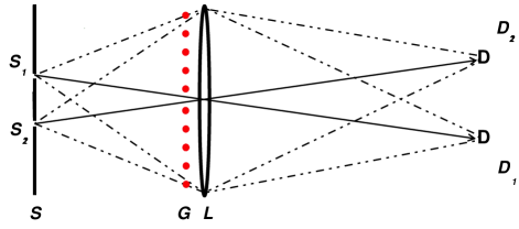
Figure 1: Setup of the ‘Afshar experiment’ Chown (2004); Afshar (2005): a double-slit $S$ is coherently and with equal intensity illuminated from the left. With the help of lens $L$ the slits’ images are recorded by detectors $D_{1}$ and $D_{2}$. At first, measurements are made without grid $G$ (dotted line); subsequently, the grid is inserted and the measurements repeated. This sketch is a slightly simplified version of the original which contains an aperture around lens $L$ and redirection mirrors in front of the detectors. Both simplifications are unimportant for the essentials of the experiment.

Stages of the experiment: in stage (i) of the experiment the grid $G$ is not present. In this stage only one slit is left open, therefore, only the corresponding detector gets illuminated. Opening of the other slit (and illuminating the other detector simultaneously) does not change the image at the first detector.

In stage (ii) the setup is modified by inserting the grid $G$ directly in front of the lens $L$, as shown in Fig. 1. The grid is carefully positioned in such a way that the wires sit at the minima of the interference pattern (which can be checked by inserting a screen at the position of $G$ and opening the second slit). It is then observed that if one of the two slits is blocked the image of the remaining open slit is strongly modified due to the presence of the grid. The wires of the grid reflect (and diffract) some of the photons, which leads to a reduction of the intensity and introduces the formation of stripes in the image of the slit Chown (2004); Afshar (2005). Note that the positioning of the grid at the minima of the interference pattern implies that it constitutes a carefully matched diffraction grating for the passing light.

In stage (iii) the other slit (previously blocked) is reopened. The crucial result at this stage is that the focal images of the two slits at detectors $D_{1}$ and $D_{2}$ look remarkably similar to those obtained in the absence of the grid in stage (i).

Afshar’s interpretation, as cited from reference Chown (2004):

• Laser light falls on two pinholes in an opaque screen. On the far side of the screen is a lens that takes the light coming through each of the pinholes (another opaque screen stops all other light hitting the lens) and refocuses the spreading beams onto a mirror that reflects each onto a separate photon detector. In this way, Afshar gets a record of the rate at which photons are coming through each pinhole. According to complementarity, that means there should be no evidence of an interference pattern. But there is, Afshar says.

  He doesn’t look at the pattern directly, but has designed the experiment to test for its presence. He places a series of wires exactly where the dark fringes of the interference pattern ought to be. Then he closes one of the pinholes. This, of course, prevents any interference pattern from forming, and the light simply spreads out as it emerges from the single pinhole. A portion of the light will hit the metal wires, which scatter it in all directions, meaning less light will reach the photon detector corresponding to that pinhole.

  But Afshar claims that when he opens up the closed pinhole, the light intensity at each detector returns to its value before the wires were set in place. Why? Because the wires sit in the dark fringes of the interference pattern, no light hits them, and so none of the photons are scattered. That shows the interference pattern is there, says Afshar, which exposes the wave-like face of light. And yet he can also measure the intensity of light from each slit with a photon detector, so he can tell how many photons pass through each slit - the particle-like face is there too.

  ”This flies in the face of complementarity, which says that knowledge of the interference pattern always destroys the which-way information and vice versa,” says Afshar. ”Something everyone believed and nobody questioned for 80 years appears to be wrong.”

In other words, stage (iii) of the experiment is interpreted as a demonstration of simultaneous ‘perfect’ particle ($D=1$) and wave behaviour ($V=1$) thus violating the complementarity inequality (1) Chown (2004); Afshar (2005).

III Wave Optical Analysis

Afshar’s interpretation relies on the fact that the slits’ images obtained in the presence of the grating, in stage (iii), are very similar to those obtained in stage (i) without a grating. In the article Chown (2004) they are describes in the figure caption of the slit images in stage (iii) of the experiment as returning to their ‘original value’, that of stage (i). But, close inspection of the images themselves reveals that in stage (iii) they display residues of the same disturbances that are seen in stage (ii) Chown (2004); Afshar (2005). These disturbances were considered negligible and without fundamental significance. Here, it is shown that these residual disturbances must not be neglected, they are key to understanding and interpreting Afshar’s experiment.

III.1 Qualitative analysis

Putting the grid into the area where the dark fringes are to be expected in stage (iii) of Afshar’s experiment is an elegant way of proving that some interference contrast is present, while quite efficiently avoiding the reflection or absorption of passing photons by the grid. But avoiding the reflection or absorption of photons is not enough to guarantee that their behaviour in relation to the complementarity principle is unaffected. The grid’s other main effect is the elastic scattering of passing (and reflected) photons due to diffraction. Even if the grid $G$ was perfectly absorbing, and hence did not reflect any photons, would it still diffract passing photons on their way from slit $S_{1}$ to detector $D_{1}$. Indeed, quite a few of those photons do get scattered towards detector $D_{2}$ because it lies in the direction of the first diffraction order of the grating, see below. For symmetry reasons, analogous perturbations affect photons on their way from slit $S_{2}$ to $D_{2}$, redirecting some towards detector $D_{1}$.

This explains some key features of Afshar’s experiment. In stage (ii) of the experiment reflection and absorption, and diffraction by the grid distort the slit images at the detectors. In stage (iii) the other slit is opened and first-order diffraction of photons from that newly opened slit apparently restores the slit images. It also shows qualitatively how the complementarity principle is at work: the path detection in the presence of the grid becomes less reliable since photons are diffracted towards the ‘wrong’ detector thus compromising path detection.

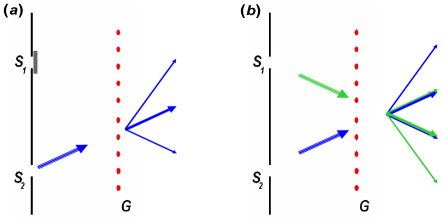
Figure 2: Geometry of wave vectors in the vicinity of the grid plane $G$: (a) only slit $S_{2}$ is open, (b) both slits are open. Some forward scattered light is deflected sideways by the grid (a). This loss of forward scattered light is partly compensated for by opening the other slit (b) which ‘adds on’ more light with the correct phase and transverse momentum. Here, only zeroth and first order transmitted light wave vectors are plotted.

III.2 Quantitative analysis of diffraction

In the forthcoming analysis we introduce three simplifications that do not affect the underlying mechanism of the experiment. Firstly, we assume the light is monochromatic with angular frequency $\omega=c\,k$ and wave number $k$, and we only analyze features in the plane defined by the optical axis and the two slits $S_{1}$ and $S_{2}$, that is, we treat the problem in two spatial dimensions. Secondly, we assume that the we can use the paraxial wave approximation, namely, we describe the light in terms of plane waves and all angles are small. Later, it will be confirmed that these two simplifications are helpful without affecting the generality of the argument. Thirdly, we model the grid by a planar reflecting film consisting of suitable strips of metal rather than an array of reflecting round wires. This last assumption would lead to a slightly better performance than Afshar’s setup, using round wires, because reflection (although not diffraction) of photons towards the ‘wrong’ detector would become completely suppressed. It also simplifies our analysis because we now encounter only two mutually exclusive subensembles of photons, transmitted and back-reflected ones.

With these simplifying assumptions we can determine the interference pattern at the grid to be proportional to $\cos(k_{\perp}x)^{2}=\cos(\frac{ks}{g}x)^{2}$, where $k$ is the wave number of the light and its transverse component $k_{\perp}=ks/g$ arises from the geometry of the setup. The distance between the slits is $2s$ and $g$ is the distance from the double-slit to the grid; small angles (paraxial beams) are assumed throughout. Consequently, the grid has spacing $\Lambda=2\pi/(2k_{\perp})=\pi g/(ks)$ and can be expanded into a Fourier-series with periodicity $\Lambda$. Our model for the grid $G(x)$ is a periodic comb of reflecting stripes; in other words, the reflectivity alternates between values of unity in regions centered at odd multiples of $\Lambda/2$ over a distance $\Lambda a,(a<1)$ and zero over the remaining distance $\Lambda(1-a)$: $a$ is the covering ratio of the grating. $G(x)$ is plotted, together with the interference pattern, in Fig. 3.

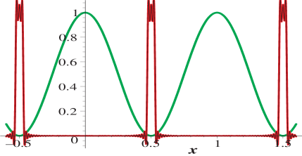
Figure 3: The grid function $G(x)$ of eq. (2) for a grid with covering ration $a=0.06$ described by a Fourier series expanded up to 50th order together with the interference pattern intensity $\cos(k_{\perp}x)^{2}$ of the two slits $S_{1}$ and $S_{2}$ in the grid plane. The $x$-axis is scaled in terms of the grid spacing $\Lambda$.

The grid’s functional description in terms of a Fourier series is given by

$$G(x) = c_{0}+\sum_{n=1}^{\infty}c_{n}\cos\left(\frac{2\pi}{\Lambda}xn\right)\;,$$ (2)

$$\mbox{with \quad}c_{0} = a,\mbox{\quad and \quad}c_{n}=2(-1)^{n}\frac{\sin(a\pi n)}{\pi n}.$$ (3)

We will now work out how this grating affects incoming plane waves. For simplicity we assume that the wave vector of the incident light $\psi_{in}$ is perpendicular to the grating. We will later include the slight deviation due to the fact that the slits $S_{1}$ and $S_{2}$ lie half a diffraction order off the optical axis. A plane wave travelling in the $z$-direction with wave vector $\vec{k}=k\;{\bf{\hat{z}}}$ is described by $\psi_{in}=e^{i(kz-\omega t)}$. When the grid diffracts this plane wave into the $n$-th positive or negative order its wave vector becomes $\vec{k}_{\pm n}=\pm k_{x,n}\;{\bf{\hat{x}}}+k_{z,n}\;{\bf{\hat{z}}}$ where $k_{x,n}=n\cdot 2k_{\perp}$ and $k_{z,n}=\sqrt{k^{2}-k_{x,n}^{2}}$.

After interaction with the grating $G$ we thus find the transmission light modes $\psi_{\pm n,t}=e^{i(k_{z,n}z\pm k_{x,n}x-\omega t)}$, and the reflection modes $\psi_{\pm n,r}=e^{i(-k_{z,n}z\pm k_{x,n}x-\omega t)}$. With the tacit understanding that the grating function (2) can be viewed as an operator $\hat{G}$ that imparts transverse momentum kicks of size $\hbar k_{x,n}=n\cdot\hbar 2k_{\perp}\doteq np_{\perp}$, we thus introduce the corresponding momentum transfer operator $\hat{p}_{\perp}$ which allows us to write down the effect of the grating on an incoming wave as

$$\hat{G}(x) = c_{0}\hat{1}+\sum_{n=1}^{\infty}c_{n}\frac{e^{i\frac{\hat{p_{\perp}}}{\hbar}xn}+e^{-i\frac{\hat{p_{\perp}}}{\hbar}xn}}{2}$$ (4)

$$= a\hat{1}+\sum_{n=1}^{\infty}\frac{(-1)^{n}\sin(a\pi n)}{\pi n}\cdot\left[e^{i\frac{\hat{p_{\perp}}}{\hbar}xn}+e^{-i\frac{\hat{p_{\perp}}}{\hbar}xn}\right].\quad$$ (5)

Including the $\pi$ phase jump associated with reflection Fey (b) we therefore find for the reflection amplitudes

$$r_{0}=-c_{0}=-a$$ (6)

and $$r_{n}=r_{-n}=\frac{-c_{n}}{2}=(-1)^{n+1}\frac{\sin(a\pi n)}{\pi n}\;.$$ (7)

Following the same logic Fey (b), we find the transmission amplitudes obey

$$t_{0}=1+r_{0}\;\mbox{ and }\;t_{n}=t_{-n}=r_{n}\;.$$ (8)

After a multiplication with $e^{i\omega t}$ to remove the time-dependence we thus arrive at the result that the reflected and transmitted partial waves have the form

$$[\psi_{t}] + [\psi_{r}]=\left[(1-c_{0})e^{ikz}-\sum_{n=1}^{\infty}\frac{c_{n}}{2}\cdot\left(\psi_{+n,t}+\psi_{-n,t}\right)\right]$$ (9)

$$- \left[c_{0}e^{-ikz}+\sum_{n=1}^{\infty}\frac{c_{n}}{2}\cdot\left(\psi_{+n,r}+\psi_{-n,r}\right)\right]\;.\quad\;$$

With $\sum_{n=1}^{\infty}c_{n}^{2}=2(a-a^{2})$ we can check the normalization and find $\sum_{n=-\infty}^{\infty}(r_{n}^{2}+t_{n}^{2})=r_{0}^{2}+t_{0}^{2}+\sum_{n=1}^{\infty}c_{n}^{2}=a^{2}+(1-a)^{2}+2(a-a^{2})=1$, as required.

After the discussion of the effect of the grating on a single plane wave $\psi_{in}=e^{i(kz-\omega t)}$ we can extend the discussion to the case of two interfering plane waves as sketched in Fig. 2 above. The transverse components $\pm\hbar k_{\perp}=\pm\Delta p_{\perp}/2$ of the incoming waves sketched in Fig. 2 (b) offset the waves by half orders up or down. This is why the diffracted (and reflected) waves fall into half odd integer orders, compare e.g. Fig. 5 (a). The partial waves of some order $n$ originating from one slit therefore overlap with the adjacent order $n-1$ or $n+1$ partial waves from the other slit.

Since amplitudes of adjacent orders have similar magnitudes but alternating signs, see eq. (7), the resulting interference is destructive: opening the second slit in stage (iii) of the experiment counteracts the perturbation due to the grating, which is so clearly visible in stage (ii). Figs. 4 and 5 illustrate the transition from stage (ii) (associated probability amplitudes $|r_{n}|^{2}$) to stage (iii) (associated amplitudes $|r_{n}+r_{n+1}|^{2}/2$). Afshar erroneously interpreted this as a ‘complete’ recovery of the slit images to their pristine form encountered in stage (i). Instead, our analysis shows that in stage (iii) light from the ‘wrong’ slit mostly compensates for the disturbances introduced by the grating in stage (ii) (although small residues of these perturbations remain, see Chown (2004); Afshar (2005) and Figs. 4 (b) and 5 (b)) but this is done at the expense of redirecting light to the ‘wrong’ detector.

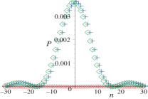
Figure 4: Reflection probabilities $P=|r_{n}^{2}|$ up to 30th order for a grid with covering ration $a=0.06$. Green diamonds and blue crosses describe the reflection probabilities for individual beams originating from slit $S_{1}$ and $S_{2}$ respectively, this corresponds to stage (ii) of the experiment, (a). When both slits are opened simultaneously the reflection is very much suppressed. One has to zoom in, (b), to see that the reflection probability $P=|r_{n}+r_{n+1}|^{2}$ (red circles) in this case is nonzero, this corresponds to stage (iii) of Afshar’s experiment.

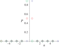
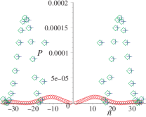
Figure 5: Transmission probabilities $P=|t_{n}^{2}|$ as in Fig. 4 above. When both slits are opened simultaneously, red circles, the diffraction into higher orders is very much suppressed (a). One has to zoom in, (b), to see that the transmission probability $P=|t_{n}+t_{n+1}|^{2}$ (red circles) is nonzero for orders higher than $\pm 1/2$.

Before closing this section let us revisit our assumptions. The monochromaticity assumption is good for the narrow-band laser light used in the experiment, the extension to temporal wave packets is straightforward, so is an extension to wider slits. The reduction to two dimensions applies to the plane depicted in Fig. 1 and to a setup with long slits rather than round holes, it does not affect the essence of the experiment. An analysis of the exact setup described in Afshar’s experiment is only more tedious but not different in principle. Modelling the grid by a planar reflecting film rather than round reflecting wires allows us to write down expressions for transmitted and reflected waves in simple form. This is obviously helpful for tracking the flow of light in this setup and in a real experiment this setup would perform better than the one used by Afshar because none of the transmitted light gets reflected towards the ‘wrong’ detector it only reaches the wrong detector via diffraction.

We can conclude that the orthodox interpretation of quantum mechanics, described in this case with the help of classical wave optics, is sufficient to analyze the experiment satisfactorily. Our analysis is also applicable to some quantum cases such as single photon, thermal or Glauber coherent light Steuernagel (2002). We will now quantify the complementarity behaviour in Afshar’s experiment.

IV Complementarity in Afshar’s experiment

The presence of the interference pattern in Afshar’s experiment is only inferred Chown (2004); Afshar (2005), but according to the orthodox interpretation of quantum mechanics it has to be measured in order to be described by the quantum mechanical operator formalism. This requirement is well captured by Wheeler’s famous dictum to the effect “that only a registered event is a real event” Whe . When studying the complementary aspects of a quantum particle’s behaviour both aspects have to be measured simultaneously for every particle Wheeler and Zurek (1983); Fey (c). How simultaneous ‘path’ and ‘wave’ measurements can be performed with Afshar’s setup is considered next.

IV.1 Qualitative discussion of complementarity

The interference pattern at the position of the grid, in stage (iii), is responsible for the reduced scattering of photons by the grid in stage (iii) of the experiment. In order to measure the contrast of the interference pattern without compromising the simultaneous path detection we have to change the relative phase $\Delta\phi$ between light emanating from the two slits (by, say, changing the relative path length between the two holes with the help of a phase shifter, or, by moving the grating) and then collect all light transmitted by the grating.

Note that transmitted and back-reflected photons form two mutually exclusive subensembles to which the complementarity principle must therefore be applied separately. In the following, just as in Afshar’s implementation of the experiment, we mostly deal with the transmitted light only, but everything we say can analogously be rephrased for the ensemble of back-reflected photons.

For transmitted light the finite slit widths of the grating reduce the observed fringe contrast because the slits of the grating are not infinitesimally small and therefore act as bucket detectors rather than as the highly spatially resolving detectors required for an ideal characterization of the interference pattern. This leads to a tradeoff between path detection and determination of the interference pattern contrast. Very narrow slits allow us to observe the modulation due to the interference pattern with great accuracy, but at the expense of strong diffraction of passing photons, thus erasing their path information. For wider slits the observed contrast of the interference pattern diminishes because wide slits sample larger parts of the interference patter denying good resolution, on the other hand the photon paths become less disturbed yielding better path information.

For reflected photons the roles are reversed since small slits correspond to wide reflecting stripes and vice versa.

IV.2 Quantification of Visibility

The light in the grating plane forms a sinusoidal field distribution, with the intensity distribution $I(x)=\cos(\frac{\pi}{\Lambda}x+\Delta\phi)^{2}$, where $\Delta\phi$ is the relative phase between the two slits $S_{1}$ and $S_{2}$. To find out how much light gets transmitted we have to integrate over the slit opening(s). We find that the transmitted intensity is given by $I_{t,max}=\int_{-\Lambda/2\cdot(1-a)}^{+\Lambda/2\cdot(1-a)}dx\;\cos(\frac{\pi}{\Lambda}x)^{2}=(\pi-a\pi+\sin(a\pi))/(2\pi)$ in the maximum case (grating positioned at interference pattern minima) and $I_{t,min}=\int_{-\Lambda/2\cdot(1-a)}^{+\Lambda/2\cdot(1-a)}dx\;\sin(\frac{\pi}{\Lambda}x)^{2}=(\pi-a\pi-\sin(a\pi))/(2\pi)$ in the minimum case (grating positioned at interference pattern maxima). The ensuing measurable visibility of transmitted light $V_{t}$ thus is

$$V_{t}(a)\doteq\frac{I_{t,max}-I_{t,min}}{I_{t,max}+I_{t,min}}=\frac{\sin(a\pi)}{\pi(1-a)}\;.$$ (10)

An analogous calculation for reflected light is easily performed and yields the expected result that the effective slit width in this case is given by $1-a$.

IV.3 Quantification of Distinguishability

For a balanced interferometric setup such as Afshar’s the distinguishability $\cal D$ of paths is determined by the power of the path detectors $D_{1}$ and $D_{2}$ to discriminate the two paths. Formally, it is given by half the distance between detector states in the trace class norm Englert (1996). Describing the light mode emanating from slit $S_{j}$ by the state $|S_{j}\rangle$ and the mode associated with detector $D_{k}$ by state $|D_{k}\rangle$ we thus have the following expression for the distinguishability of transmitted light ${\cal D}_{t}$ Englert (1996)

$${\cal D}_{t}(a) = \frac{1}{2}\sum_{j=1}^{2}\left||\langle S_{j}|D_{1}\rangle|^{2}-|\langle S_{j}|D_{2}\rangle|^{2}\right|$$ (11)

$$= \frac{1}{2}\left(\left||t_{0}|^{2}-|t_{1}|^{2}\right|+\left||t_{1}|^{2}-|t_{0}|^{2}\right|\right)$$ (12)

$$= (1-a)^{2}-\left(\frac{\sin(a\pi)}{\pi}\right)^{2}\,.$$ (13)

IV.4 Quantification of Complementarity

Combining these results allows us to see that

$${\cal D}_{t}^{2}(a)+V_{t}^{2}(a)\leq 1\,,$$ (14)

where the limit of unity is only reached for the extreme cases of $a=0$ (complete absence of a grid) or $a=1$ (complete covering by a plane mirror that reflects all light and thus allows us to discriminate the slits perfectly when utilizing the back-reflected light), see Fig 6.

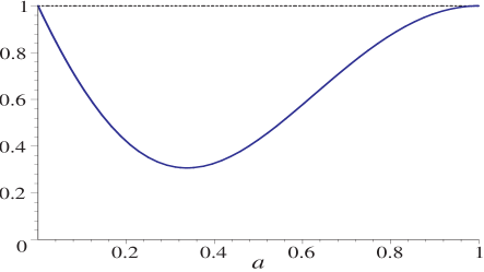
Figure 6: Complementarity is never violated in Afshar’s experiment: ${\cal D}_{t}^{2}(a)+V_{t}^{2}(a)\leq 1$ for all covering ratios $a$.

IV.5 Some difficulties with Afshar’s experiment

Before we conclude let us mention some subtleties of the Afshar experiment which could be quantified – if one was so inclined.

The experiment is not very well designed to perform complementarity experiments because the amount of transmitted and reflected light depends on the relative position of the grating with respect to the interference pattern. For energy conservation reasons, the less light gets transmitted ($I_{t,min}$) the more gets reflected and vice versa. This behaviour, in some sense connects the subensemble of transmitted light with that of the reflected light. Not in the sense that one subensemble allows us to infer anything about the complementarity behaviour of the other but in the sense that a more detailed analysis would have to introduce weighting factors. This is an unwelcome complication I neglected in my analysis.

Another weakness of the setup are losses, partly due to the use of round wires in Afshar’s implementation. But even in the simpler version discussed here, we still encounter losses into higher diffraction orders. Although they could be included into the analysis they only diminish the path-resolution further and the experimental setup would become more involved.

Finally, the greatest weakness in the analysis given by Afshar is the inference that an interference pattern must be present. Quantum mechanics is not an ontological theory, it must not be approached as such, only measured events are described by quantum mechanics Whe ; Fey (c).

V Conclusion

The quantification of the principle of complementarity in section IV shows that Afshar’s experiment must not be interpreted as an example of a possible violation of the principle of complementarity of quantum mechanics. It is actually suboptimal in the sense that it does not fully exhaust the limits stipulated by quantum mechanics; unlike, say, the nearly optimal experiment performed by Dürr et al. Dürr et al. (1998).