Fault-Tolerant Landau-Zener Quantum Gates

Abstract

We present a method to perform fault-tolerant single-qubit gate operations using Landau-Zener tunneling. In a single Landau-Zener pulse, the qubit transition frequency is varied in time so that it passes through the frequency of the radiation field. We show that a simple three-pulse sequence allows eliminating errors in the gate up to the third order in errors in the qubit energies or the radiation frequency.

I Introduction

In many proposed implementations of a quantum computer (QC) single-qubit operations are performed by applying pulses of radiation. The pulses cause resonant transitions between qubit states, that is between the states of the system that comprises a qubit. The operation is determined by the pulse amplitude and duration. In many proposals, particularly in the proposed scalable condensed-matter based systems Kane (1998), control pulses will be applied globally, to many qubits at a time. A target qubit is chosen by tuning it in resonance with the radiation. The corresponding gate operations invariably involve errors which come from the underlying errors in the frequency, amplitude, and length of the radiation pulse as well as in the qubit tuning.

Improving the accuracy of quantum gates and reducing their sensitivity to errors from different sources is critical for a successful operation of a QC. Much progress has been made recently in this direction by using radiation pulses of special shape and composite radiation pulses Vandersypen and Chuang (2004). In the analysis or resonant pulse shape it is usually assumed that the qubit transition frequency is held constant during the pulse.

An alternative approach to single-qubit operations is based on Landau-Zener tunneling (LZT) Landau (1932); Zener (1932). In this approach the qubit transition frequency $\omega_{0}(t)$ is swept through the frequency of the resonant field $\omega_{F}$ Dykman and Platzman (2001). The change of the qubit state depends on the field strength and the speed at which $\omega_{0}(t)$ is changed when it goes through resonance Benza and Strini (2003). The LZT can be used also for a two-qubit operation in which qubit frequencies are swept past each other leading to excitation swap Dykman and Platzman (2001); Platzman and Dykman (1999); Saito and Kayanuma (2004).

In the present paper we study the robustness of the LZT-based gate operations. We develop a simple pulse sequence that is extremely stable against errors in the qubit transition frequency or equivalently, the radiation frequency. Such errors come from various sources. An example is provided by systems where the qubit-qubit interaction is not turned off, and therefore the transition energy of a qubit depends on the state of other qubits. Much effort has been put into developing means for correcting them using active control Viola (2004); Facchi et al. (2005); Sengupta and Pryadko (2005).

An advantageous feature of LZT is that the change of the qubit state populations depends on the radiation amplitude and the speed of the transition frequency change $\dot{\omega}_{0}$, but not on the exact instant of time when the frequency coincides with the radiation frequency, $\omega_{0}(t)=\omega_{F}$. However, the change of the phase difference between the states depends on this time. Therefore an error in $\omega_{0}$ or $\omega_{F}$ leads to an error in the phase difference, i.e., a phase error. This error has two parts: one comes from the phase accumulation before crossing the resonant frequency, and the other after the crossing. Clearly, they have opposite signs.

A natural way of reducing a phase error is to make the system accumulate the appropriate opposite in sign phases before and after the “working” pulse. To do this, we first apply a strong radiation pulse that swaps the states, which can be done with exponentially high efficiency using LZT. Then we apply the “working” pulse, and then another swapping pulse. The swapping pulses effectively change the sign of the accumulated phase. As we show, by adjusting their parameters we can compensate phase errors with a high precision.

In Sec. II below we give the scattering matrix for LZT in a modified adiabatic basis which turns out to be advantageous compared to the computational basis. The scattering matrix describes the quantum gate. In Sec. III it is presented in more conventional for quantum computation terms of the qubit rotation matrix. In Sec. IV, which is the central part of the paper, we propose a simple composite Landau-Zener (LZ) pulse and demonstrate that it efficiently compensates energy offset errors even where these errors are not small. Sec. V contains concluding remarks.

II Landau-Zener transformation in the modified adiabatic basis

A simple implementation of the LZ gate is as follows. The amplitude of the radiation pulse is held fixed, while the difference between the qubit transition frequency and the radiation frequency

$$\Delta=\Delta(t)=\omega_{F}-\omega_{0}(t)$$ (1)

is swept through zero. If $\omega_{0}(t)$ is varied slowly compared to $\omega_{F}$, i.e., $|\dot{\omega}_{0}|\ll\omega_{F}^{2}$, the qubit dynamics can be described in the rotating wave approximation, with Hamiltonian

$$H=H(t)=\left(\begin{array}[]{cc}\Delta/2&\gamma\\ \gamma&-\Delta/2\end{array}\right).$$ (2)

Here, $\gamma$ is the matrix element of the radiation-induced interstate transition. The Hamiltonian $H$ is written in the so-called computational basis, with wave functions $\left|0\right\rangle=\left(\begin{array}[]{c}1\\ 0\end{array}\right)$ and $\left|1\right\rangle=\left(\begin{array}[]{c}0\\ 1\end{array}\right)$.

We assume that well before and after the frequency crossing the values of $|\Delta|$ largely exceed $\gamma$ and $\Delta$ slowly varies in time, $|\dot{\Delta}/\Delta^{2}|\ll 1$. Then the wave functions of the system are well described by the adiabatic approximation, i.e., by the instantaneous eigenfunctions of the Hamiltonian (2),

$$\left|{\psi_{0}}\right\rangle=\left[\begin{array}[]{c}\cos(\theta/2)\\ \sin(\theta/2)\end{array}\right],\qquad\left|{\psi_{1}}\right\rangle=\left[\begin{array}[]{c}-\sin(\theta/2)\\ \cos(\theta/2)\end{array}\right],$$ (7)

$$\theta=({\rm sgn}\Delta)\cos^{-1}\frac{|\Delta|}{2E},\qquad E=\left(\frac{\Delta^{2}}{4}+\gamma^{2}\right)^{1/2},$$

where $\Delta\equiv\Delta(t)$ and $(-1)^{n}E\,{\rm sgn}\Delta$ is the adiabatic energy of the states $|\psi_{n}\rangle=|\psi_{0,1}\rangle$. The adiabatic approximation for $E$ and $\theta$ is accurate to $\gamma^{2}\dot{\Delta}/\Delta^{3}$ and $\gamma\dot{\Delta}/\Delta^{3}$, respectively.

In contrast to the standard adiabatic approximation, we chose the states $|\psi_{0,1}\rangle$ and their energies in such a way that $|\psi_{0}\rangle$ and $|\psi_{1}\rangle$ go over into $|0\rangle$ and $|1\rangle$, respectively, for $|\Delta|/\gamma\to\infty$. As a result $\theta$ is discontinuous as a function of $\Delta$ for $\Delta=0$, but the adiabatic approximation does not apply for such $\Delta$ anyway.

For the future analysis it is convenient to introduce the Pauli matrices $X,Y,Z$ in the basis (7), with

$$Z|\psi_{n}\rangle=(1-2n)|\psi_{n}\rangle,\qquad X|\psi_{n}\rangle=|\psi_{1-n}\rangle\quad(n=0,1),$$

and $Y=iXZ$. In these notations, the operator of the adiabatic time evolution $U(t_{f},t_{i})=T\exp[-i\int\nolimits_{t_{i}}^{t_{f}}dtH(t)]$ has the form

$$U(t_{f},t_{i})=\exp\left[-i\left({\rm sgn}\,\Delta\right)Z\,\int_{t_{i}}^{t_{f}}E(t)\,dt\right],$$ (8)

with ${\rm sgn}\,\Delta\equiv{\rm sgn}\,\Delta(t_{i})\equiv{\rm sgn}\,\Delta(t_{f})$ [the sign of $\Delta(t)$ is not changed in the range where Eq. (8) applies].

The LZ transition can be thought of as occurring between the states (7). Following the standard scheme Landau (1932); Zener (1932) we take two values $\Delta_{1,2}$ of $\Delta(t)$ such that they have opposite signs, $\Delta_{1}\Delta_{2}<0$. We choose $|\Delta_{1,2}|$ sufficiently large, so that the adiabatic approximation (7) applies for $\Delta(t_{i})=\Delta_{i},i=1,2$. At the same time, $|\Delta_{1,2}|$ are sufficiently small, so that $\Delta(t)$ can be assumed to be a linear function of time between $\Delta_{1}$ and $\Delta_{2}$,

$$\Delta(t)\approx-\eta(t-t_{c}),\qquad\eta=-\dot{\Delta}(t_{c}),$$ (9)

where the crossing time $t_{c}$ is given by the condition $\Delta(t_{c})=0$. The adiabaticity for $t=t_{1,2}$ requires that $|\Delta_{1,2}|\gg\gamma,\eta^{1/2}$. We will consider the LZ transition first for the case $\Delta_{1}>0$ and $\Delta_{2}<0$, when $\eta>0$.

The modified adiabatic basis (7) is advantageous, because in this basis the transition matrix $S$ has a particularly simple form. For $\Delta(t)$ of the form (9) the error in $S$ is determined by the accuracy of the adiabatic approximation itself and is of order $\gamma/\eta^{2}|t_{1,2}-t_{c}|^{3}$, in contrast to the computational basis, where the error is $\sim O(\gamma/\eta|t_{1,2}-t_{c}|)$. This latter error is comparatively large for the values of $\gamma/|\Delta_{1,2}|$ of interest for quantum computing. It leads to the well-known oscillations of the transition amplitude with increasing $|\Delta|$ Benza and Strini (2003), whereas in the basis (7) such oscillations do not arise, see Fig.1.

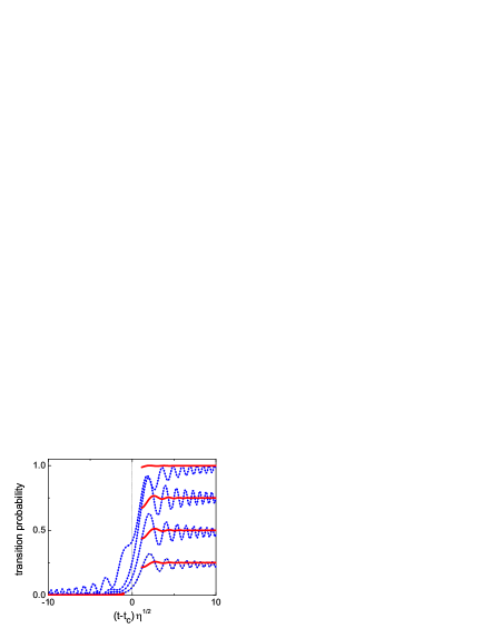
Figure 1: (Color online). Landau-Zener transitions $|\psi_{0}\rangle\to|\psi_{1}\rangle$ and $|0\rangle\to|1\rangle$ in the modified adiabatic basis (7) and in the computational basis for linear $\Delta(t)$ (9). Solid and dotted lines show the squared amplitude of the initially empty states $|\psi_{1}\rangle$ and $|1\rangle$, respectively. The data for the state $|\psi_{1}\rangle$ close to $\Delta(t)=0$ are not shown, since the adiabatic approximation does not apply for small $|\Delta|$. The lines refer to $g=1,0.47,0.33,$ and $0.21$, in the order of decreasing transition probability for $(t-t_{c})\eta^{1/2}=10$. As long as $\Delta(t)$ is large and negative, the system stays in the initially occupied adiabatic state $|\psi_{0}\rangle$, and therefore the solid curves for different $g$ cannot be resolved for $(t-t_{c})\eta^{1/2}\lesssim-1$. For large $(t-t_{c})\eta^{1/2}$ the solid lines quickly approach the Landau-Zener probabilities $1-e^{-2\pi g^{2}}$.

The energy detuning $|\Delta_{1,2}|$ cannot be made too large, because this would make the gate operation long. If we characterize the overall error of the adiabatic approximation as the sum $\sum\nolimits_{i=1,2}\gamma/\eta^{2}|t_{i}-t_{c}|^{3}$ and impose the condition that the overall duration of the operation $t_{2}-t_{1}$ be minimal, we see that the error is minimized when the pulses $\Delta(t)$ are symmetrical, $t_{2}-t_{c}=t_{c}-t_{1}$, i.e., $|\Delta_{1}|=|\Delta_{2}|$.

The matrix $S(t_{2},t_{1})\equiv S$ in the basis (7) can be obtained using the parabolic cylinder functions that solve the Schrödinger equation with the Hamiltonian (2), (9),

$$S(t_{2},t_{1})=\left(\begin{array}[]{cc}\exp\left[-\pi g^{2}+i(\varphi_{2}-\varphi_{1})\right]&-\frac{(2\pi)^{1/2}}{g\,\Gamma\left(ig^{2}\right)}\exp\left[-\frac{\pi}{2}g^{2}-i\frac{\pi}{4}+i(\varphi_{1}+\varphi_{2})\right]\\ \frac{(2\pi)^{1/2}}{g\,\Gamma\left(-ig^{2}\right)}\exp\left[-\frac{\pi}{2}g^{2}+i\frac{\pi}{4}-i(\varphi_{1}+\varphi_{2})\right]&\exp\left[-\pi g^{2}-i(\varphi_{2}-\varphi_{1})\right]\end{array}\right),$$ (10)

where $\Gamma(x)$ is the gamma function.

The dimensionless coupling parameter $g=\gamma/|\eta|^{1/2}$ in Eq. (10) is the major parameter of the theory, it determines the amplitude of the $|\psi_{n}\rangle\to|\psi_{1-n}\rangle$ transition. The phases $\varphi_{1,2}$ are

$$\varphi_{i}=\frac{\Delta_{i}^{2}}{4|\eta|}+g^{2}\ln\left(\frac{|\Delta_{i}|}{|\eta|^{1/2}}\right)+\frac{g^{4}|\eta|}{2\Delta_{i}^{2}},\qquad i=1,2.$$ (11)

Here we have disregarded the higher order terms in $|\Delta_{1,2}|^{-1}$. The constants in $\varphi_{1,2}$ are chosen so as to match the corresponding constants in the parabolic cylinder functions Gradshteyn and Ryzhik (2000).

The matrix $S$ for a transition from the initial state with $\Delta_{1}<0$ to the final state with $\Delta_{2}>0$ is given by the transposed matrix (10) in which the phases $\varphi_{1}$ and $\varphi_{2}$ are interchanged. In this case $\eta<0$ in Eq. (9); the expressions for $\varphi_{1,2}$ and $g$ do not change.

III Rotation matrix representation

The LZ transition can be conveniently described using the standard language of gate operations in quantum computing. To do this we express the transition matrix in terms of the operators $R_{X}(\theta)=\exp(-i\theta X/2)$ and $R_{Z}(\theta)=\exp(-i\theta Z/2)$ of rotation about $x$ and $z$ axes in the basis (7). The rotation matrices can be written using the “adiabatic” phases $\phi(t_{i})$ that accumulate between the time $t_{i}$ and the time $t_{c}$ at which the levels would cross in the absence of coupling. From Eq. (11)

$$\varphi_{i}=\phi(t_{i})+\varphi_{0}\quad(i=1,2),\qquad t_{1}<t_{c}<t_{2},$$

$$\phi(t_{i})=\left|\int_{t_{c}}^{t_{i}}E\,dt\right|,\qquad\varphi_{0}=\frac{1}{2}g^{2}(\ln g^{2}-1),$$ (12)

where we have disregarded corrections $\propto|\Delta_{1,2}|^{-4}$, in agreement with the approximations made in obtaining Eq. (10).

For the case $\Delta_{1}>0>\Delta_{2}$ the dependence of the transition matrix $S$ (10) on the phases $\phi(t_{1,2})$ has the form

$$S(t_{2},t_{1})=R_{z}\left[-2\phi(t_{2})\right]S^{\prime}R_{z}\left[2\phi(t_{1})\right].$$ (13)

A direct calculation shows that the matrix $S^{\prime}$ is

$$S^{\prime}=R_{z}(\Phi)R_{x}(\alpha)R_{z}(-\Phi).$$ (14)

The rotation angles $\Phi,\alpha$ are given by the expressions

$$\Phi=-2\varphi_{0}+\arg\Gamma(ig^{2})+\frac{3\pi}{4},$$ (15)

$$\alpha=2\cos^{-1}\left[\exp(-\pi g^{2})\right].$$

A minor modification of these equations allows using them also for the case $\Delta_{1}<0<\Delta_{2}$ when the frequency difference is increased in time in order to bring the states in resonance. It was explained below Eq. (11) how to relate the matrix $S$ in this case to the matrix $S$ for $\Delta_{1}>0>\Delta_{2}$. Following this prescription we obtain

$$S(t_{2},t_{1})=R_{z}\left[2\phi(t_{2})-\Phi\right]R_{x}(\alpha)R_{z}\left[-2\phi(t_{1})+\Phi\right].$$ (16)

In the rotation matrix representation, the only difference from the $S$ matrix from the case of decreasing $\Delta(t)$ is that $\Phi$ and $\phi(t_{1,2})$ change signs.

Figure 2: (Color online). The rotation angles $\alpha$ (solid line) and $\Phi$ (dashed line) in the rotation-matrix representation of the Landau-Zener gate operation as functions of the control parameter $g$. The $\pi/2$ gate, $\alpha=\pi/2$, requires $g=[\ln 2/(2\pi)]^{-1/2}\approx 0.33$.

Eqs. (13)-(16) express the LZ transition matrix in the form of rotation operators in the basis of the modified adiabatic states $|\psi_{0}\rangle$ and $|\psi_{1}\rangle$ (7). For strong coupling, $\exp(-\pi g^{2})\ll 1$, the rotation angle $\alpha$ approaches $\pi$, which corresponds to a population swap between the adiabatic states. It is well known from the LZ theory Landau (1932); Zener (1932) that the swap operation is exponentially efficient, $\pi-\alpha\approx 2\exp(-\pi g^{2})$ for large $g$. In the opposite limit of weak coupling, $g\ll 1$, the change of the state populations is small, $\alpha\approx(8\pi)^{1/2}g$. In addition to the change of state populations there is also a phase shift that accumulates during an operation. The dependence of the angles $\alpha$ and $\Phi$ on the coupling parameter $g$ is shown in Fig.2.

IV Composite Landau-Zener pulses

For many models of quantum computers an important source of errors are errors in qubit transition frequencies $\omega_{0}$. They may be induced by a low-frequency external noise that modulates the interlevel distance. They may also emerge from errors in the control of the qubit-qubit interaction: if the interaction is not fully turned off between operations, the interlevel distance is a function of the state of other qubits. In addition there are systems where the interaction is not turned off at all, like in liquid state NMR-based QC’s. In all these systems it is important to be able to perform single-qubit gate operations that would be insensitive to the state of other qubits.

The rotation-operator representation suggests a way to develop fault tolerant composite LZ pulses with respect to errors in the qubit transition frequency $\omega_{0}$ and in the radiation frequency $\omega_{F}$. We will assume that there is a constant error $\varepsilon$ in the frequency difference $\Delta(t)=\omega_{F}-\omega_{0}(t)$, but that no other errors occur during the gate operation. From Eq. (9), the renormalization $\Delta(t)\to\Delta(t)+\varepsilon$ translates into the change of the adiabatic energy $E$ and the crossing time $t_{c}$, with $t_{c}\to t_{c}+\varepsilon/\eta$. As a result the phases $\phi(t_{1,2})$ as given by Eq. (III) are incremented by

$$\delta\phi(t_{i})=\frac{E(t_{i})\Delta(t_{i})}{|\eta\Delta(t_{i})|}\varepsilon+\frac{|\Delta(t_{i})|}{8|\eta|E(t_{i})}\varepsilon^{2},\qquad i=1,2,$$ (17)

to second order in $\varepsilon$.

IV.1 Error compensation with $\pi$-pulses

A simple and robust method of compensating errors in $\phi$ is based on a composite pulse that consists of the desired pulse sandwiched between two auxiliary pulses. Using $\pi$-pulses in which $\Delta(t)$ is linear in $t$, as shown in Fig. 3, it is possible to eliminate errors of first and second order in $\varepsilon$. The goal is to compensate the factors $R_{z}[\pm 2\delta\phi(t_{1,2})]$ in the $S$-matrix (13). We note that all other factors in $S$ are not changed by the energy change $\varepsilon$, which is one of the major advantageous features of the LZ gate operation. A $\pi$-pulse is obtained if $\exp(\pi g^{2})\gg 1$, which is met already for not too large $g$: for example, $\exp(-\pi g^{2})<10^{-5}$ for $g>1.92$.

Disregarding corrections $\sim\exp(-\pi g^{2})$ we can write the $S$-matrix for the $\pi$-pulse as

$$S_{\pi}(t^{\prime},t) \approx -iXR_{z}[2\phi_{\pi}(t)+2\phi_{\pi}(t^{\prime})-2\Phi]$$ (18)

$$\equiv-iR_{z}[-2\phi_{\pi}(t)-2\phi_{\pi}(t^{\prime})+2\Phi]X,$$

where $t,t^{\prime}$ are the initial and final times, and the subscript $\pi$ indicates that the corresponding quantities refer to a $\pi$-pulse. We assume that $\Delta(t)>0>\Delta(t^{\prime})$.

The overall gate operation is now performed by a composite pulse

$$S_{c}(t^{\prime}_{2},t^{\prime}_{1})=S_{\pi}(t^{\prime}_{2},t_{2})S(t_{2},t_{1})S_{\pi}(t_{1},t^{\prime}_{1}).$$ (19)

In writing this expression we assumed that the system is switched instantaneously between the states that correspond to the end (beginning) of the correcting pulse and the beginning (end) of the working pulse $S(t_{2},t_{1})$. The overall composite pulse is shown in Fig. 3.

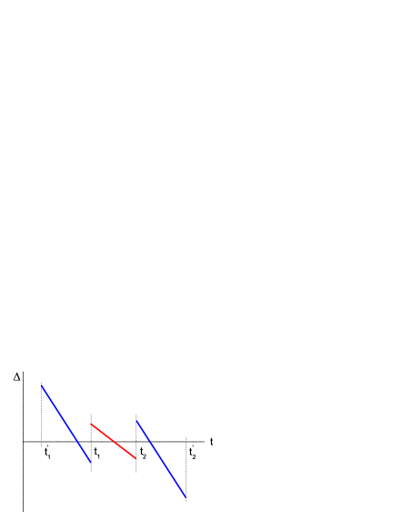
Figure 3: (Color online). An idealized composite pulse. The first and third pulses are $\pi$-pulses, the pulse in the middle performs the required gate operation. The overall pulse compensates errors in the qubit energy to 3rd order.

The first and the second $\pi$-pulses correct the errors $\delta\phi$ (17) in the phases $\phi(t_{1})$ and $\phi(t_{2})$, respectively. We show how it works for $\phi(t_{2})$. From Eqs. (13), (18), the error in $\phi(t_{2})$ will be compensated if

$$\delta\phi_{\pi}(t^{\prime}_{2})+\delta\phi_{\pi}(t_{2})-\delta\phi(t_{2})=0.$$

To second order in $\varepsilon$, the errors $\delta\phi$ here are given by Eq. (17) with appropriate $t_{i}$. The total error will be equal to zero provided

$$\frac{E_{\pi}(t^{\prime}_{2})}{\eta_{\pi}}-\frac{E(t_{2})}{\eta}-\frac{E_{\pi}(t_{2})}{\eta_{\pi}}=0,$$

$$\frac{|\Delta_{\pi}(t^{\prime}_{2})|}{\eta_{\pi}E_{\pi}(t^{\prime}_{2})}-\frac{|\Delta(t_{2})|}{\eta E(t_{2})}+\frac{\Delta_{\pi}(t_{2})}{\eta_{\pi}E_{\pi}(t_{2})}=0.$$ (20)

Equations (IV.1) are simplified if we keep only the lowest order terms with respect to $\gamma^{2}/\Delta^{2}$, in which case $E(t_{i})\approx|\Delta(t_{i})|/2$ both for the working and the correcting pulse. This gives

$$\eta_{\pi}=2\eta,\qquad|\Delta_{\pi}(t^{\prime}_{2})|-2|\Delta(t_{2})|-\Delta_{\pi}(t_{2})=0.$$ (21)

An immediate consequence of Eq. (21) is that the coupling constant $\gamma_{\pi}$ for the $\pi$-pulse should exceed the value of $\gamma$ for the working pulse, because $g_{\pi}\geq g$ and $\eta_{\pi}>\eta$. Another consequence is that the $\pi$-pulse amplitude should exceed that of the working pulse. If we choose $\Delta_{\pi}$ so that the error of the adiabatic approximation in the $\pi$-pulse does not exceed that of the working pulse, $\gamma_{\pi}\eta_{\pi}/|\Delta_{\pi}|^{3}\leq\gamma\eta/|\Delta(t_{2})|^{3}$, we obtain from Eq. (21) the condition $\Delta_{\pi}(t_{2})\geq|\Delta(t_{2})|2^{1/2}(g_{\pi}/g)^{1/3}$.

We note that the correcting pulse is asymmetric, with $|\Delta_{\pi}(t^{\prime}_{2})|>\Delta_{\pi}(t_{2}),2|\Delta(t_{2})|$, as shown in Fig. 3. Another important comment is that the proposed simple single pulse does not allow us to correct errors of higher order in $\varepsilon$. It is straightforward to see that the equation for $\Delta_{\pi}(t_{2}),\Delta_{\pi}(t_{2}^{\prime})$ that follows from the condition that the error $\sim\varepsilon^{3}$ vanishes is incompatible with Eqs. (21). However, the terms $\propto(\varepsilon/\gamma)^{3}$ contain a small factor $g^{2}\gamma/\Delta(t_{1,2})^{3}\ll 1$. The higher-order terms in $\varepsilon/\gamma$ contain higher powers of the parameter $\gamma/\Delta(t_{1,2})$. This is why compensating errors only up to the second order in $\varepsilon$ turns out efficient.

The analysis of the first correcting $\pi$-pulse, $S_{\pi}(t_{1},t_{1}^{\prime})$, is similar to that given above. The amplitude of this pulse also exceeds the amplitude of the working pulse. The duration of the correcting pulses is close to the duration of the working pulse, for $g\sim 1$ and $g_{\pi}\gtrsim 2$.

The pulse sequence (19) is written assuming that the radiation is switched off between the pulses and that the switching between the working and correcting pulses is instantaneous. A generalization to a more realistic case of a nonzero switching time is straightforward. The time evolution between the pulses can be described by extra terms in the phases $\phi_{\pi}(t_{1}),\phi_{\pi}(t_{2})$, leading to the appropriate modification of the equations for error compensation (IV.1). The analysis can be also extended to the case where $\Delta(t)$ is a nonlinear function of time and the coupling $g$ depends on time. This extension requires numerical analysis; we have found for several types of $\Delta(t),g(t)$ that good error correction can still be achieved with a three-pulse sequence.

IV.2 Maximal error of the three-pulse sequence

In order to demonstrate the error correction we will consider single working pulses $S(t_{2},t_{1})$ with the overall phases ${\Phi-2\phi(t_{1,2})\equiv 0\,({\rm mod}\,2\pi)}$ in the absence of errors, which we will denote by $S^{(0)}(t_{2},t_{1})$. Such pulses describe transformations between the states (7) with no extra phase, that is pure $X$ rotations. We will also choose the correcting $\pi$-pulses with the overall phase ${2\phi_{\pi}(t)+2\phi(t^{\prime})-2\Phi\equiv 0\,({\rm mod}\,2\pi)}$ in the absence of errors, with $t,t^{\prime}$ being $t_{1}^{\prime},t_{1}$ and $t_{2},t_{2}^{\prime}$ for the first and second pulse, respectively. Then in the absence of errors the overall gate is either not affected by the correcting pulse or its sign is changed.

The restriction on the phases provides extra constraints on the parameters of the correcting pulses. First of all, it ”discretizes” the total duration of the pulses. For the correcting pulses we still have a choice of $\Delta_{\pi}(t_{2})$ and $\Delta_{\pi}(t_{1})$. They will be chosen maximally close to $|\Delta(t_{2})|2^{1/2}(g_{\pi}/g)^{1/3}$ and $\Delta(t_{1})2^{1/2}(g_{\pi}/g)^{1/3}$, respectively, in order to minimize the error of the adiabatic approximation (7) and to minimize the overall pulse duration.

We will characterize the gate error ${\cal E}$ by the spectral norm of the difference of the operator $S$ in the presence of errors and the “ideal” gate operator $S^{(0)}$,

$${\cal E}=||S-S^{(0)}||_{2}.$$ (22)

Here, $||A||_{2}$ is the square root of the maximal eigenvalue of the operator $A^{\dagger}A$. For uncorrected pulses $S=S(t_{2},t_{1})$, whereas for corrected pulses $S=S_{c}(t_{2}^{\prime},t_{1}^{\prime})$. For simple symmetric composite pulses described below, the overall sign of the composite pulse is opposite to that of the original pulse in the absence of errors. In this case we set $S=-S_{c}(t_{2}^{\prime},t_{1}^{\prime})$ in Eq. (22).

For uncorrected pulses we have

$${\cal E}=2^{1/2}|1-n_{x1}n_{x2}-n_{y1}n_{y2}\cos\alpha|^{1/2},$$ (23)

where ${\bf n}_{i}=(\cos[\delta\phi(t_{i})],\sin[\delta\phi(t_{i})])$ is an auxiliary 2D unit vector ($i=1,2$). Eq. (22) applies also in the case of corrected pulses, but now we have to replace in the definition of the ${\bf n}_{1}$ vector

$$\delta\phi(t_{1})\rightarrow\delta\phi(t_{1})-\delta\phi_{\pi}(t_{1})-\delta\phi_{\pi}(t_{1}^{\prime}).$$ (24)

A similar replacement must be done in the definition of the vector ${\bf n}_{2}$.

For small phase errors $|\delta\phi(t_{1,2})|$ the function ${\cal E}$ for uncorrected pulses is linear in the error. In particular, to first order in $\varepsilon$ for a symmetric pulse we have $|\delta\phi(t_{1})|\approx|\delta\phi(t_{2})|\approx\varepsilon E(t_{1})/\eta$, and ${\cal E}\approx 2|\varepsilon|E(t_{1})\eta^{-1}\sin(\alpha/2)$. In contrast, by applying the same arguments to a corrected pulse, we see that the gate error is $\propto\varepsilon^{3}$. As noted above, the terms $\propto\varepsilon^{3}$ and higher-order terms in $\varepsilon$ contain a small factor. They become very small already for not too small $\varepsilon$.

To illustrate how the composite pulse works we compare in Fig. 4 the error of an uncorrected LZ gate with the gate error of the composite pulse. The data refer to different values of $g$ of the working pulse; the corresponding values of $\alpha$ are given in Fig. 2. We used $\Delta(t_{1})=-\Delta(t_{2})\approx 10\eta^{1/2}$ [the precise value of $\Delta(t_{1,2})$ was adjusted to make $S(t_{2},t_{1})$ an $X$-rotation, $S(t_{2},t_{1})=R_{x}(\alpha)$]. The compensating $\pi$-pulses where modeled by pulses with $g_{\pi}=3$. Based on the arguments provided at the end of Sec. IV A, we took $\Delta_{\pi}(t_{2})\approx|\Delta(t_{2})|2^{1/2}(g_{\pi}/g)^{1/3}$, whereas $\Delta_{\pi}(t_{2}^{\prime})$ was found from Eq. (IV.1); we used $\Delta_{\pi}(t_{1}^{\prime})=-\Delta_{\pi}(t_{2}^{\prime})$ and $\Delta_{\pi}(t_{1})=-\Delta_{\pi}(t_{2})$.

It is seen from Fig. 4 that the proposed composite pulses are extremely efficient for compensating gate errors. Even for the energy error $\varepsilon=\gamma$, where the error of an uncorrected pulse is close to 1, for the composite pulse ${\cal E}\lesssim 10^{-3}$. For $g\lesssim 1$ the error of the single pulse scales as $\varepsilon$, whereas the error of the composite pulse scales as $\varepsilon^{3}$, in agreement with the theory. For large $g$, when the gate is almost an $X$-gate ($\pi$-pulse), in the case of symmetric pulses that we discuss, the coefficients at the terms $\propto\varepsilon$ and $\propto\varepsilon^{3}$ become small; they become equal to zero for $\alpha=\pi$. Therefore for large $g$ and for not too small $\varepsilon$ the errors of single and composite pulses scale as $\varepsilon^{2}$ and $\varepsilon^{4}$, respectively. On the other hand, for $\varepsilon/\gamma$ close to 1, errors of the composite pulses with larger $g$ are larger than for smaller $g$. This is because the calculations in Fig. 4 refer to the same $\Delta/\eta^{1/2}$, in which case the errors $\propto\varepsilon^{3},\varepsilon^{4}$ are proportional to $g^{2}$.

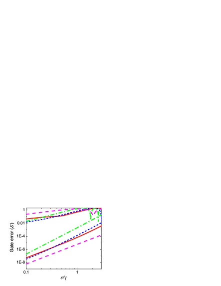
Figure 4: (Color online). Gate errors ${\cal E}$ for Landau-Zener pulses as a function of the frequency error $\varepsilon$. The upper and lower curves refer to the single LZ pulse and the composite pulse, respectively. The dash-dotted, dotted, solid, and dashed lines show ${\cal E}$ for $g=2,1.2,1$, and $0.3$.

V Conclusions

In this paper we have developed a theory of quantum gates based on LZ pulses. In these pulses the control dc field is varied in such a way that the qubit frequency passes through the frequency of the external radiation field. In the adiabatic basis an LZ gate can be expressed in a simple explicit form in terms of rotation matrices. Our central result is that already a sequence of three LZ pulses can be made fault-tolerant. The error of the corresponding composite pulse ${\cal E}$ scales with the error $\varepsilon$ in the qubit energy or radiation frequency at least as $\varepsilon^{3}$. In addition, the coefficient at $\varepsilon^{3}$ has an extra parametrically small factor. The duration of the 3-pulse sequence is about 4 times the duration of the single pulse, for the parameters that we used.

Fault tolerance of LZ gates is partly due to the change of state populations being independent of precise frequency tuning. In particular, LZ tunneling makes it possible to implement simple $\pi$-pulses with an exponentially small error in the state population.

The approach developed here can be easily generalized to more realistic smooth pulses, as mentioned above. It can be applied also to two-qubit gate operations in which the frequencies of interacting qubits are swept past each other, leading to excitation transfer Dykman and Platzman (2001). Such operations are complementary to two-qubit phase gates and require a different qubit-qubit interaction.

LZ pulses provide an alternative to control pulses where qubits stay in resonance with radiation for a specified time Vandersypen and Chuang (2004). In this more conventional approach it is often presumed that qubits are addressed individually by tuning their frequencies. In contrast to this technique, LZ pulses do not require stabilizing the frequency at a fixed value during the operation. As a consequence, calibration of LZ pulses is also different, which may be advantageous for some applications, in particular in charge-based systems Platzman and Dykman (1999); Smelyanskiy et al. (2005). The explicit expressions discussed above require that the qubit transition frequency vary linearly with time, but the linearity is needed only for a short time when the qubit and radiation frequencies are close to each other, as seen from Fig.1, which should not be too difficult to achieve.

For pulses based on resonant tuning for a fixed time, much effort has been put into developing fault-tolerant pulse sequences, see Ref. Brown et al., 2004 and papers cited therein. In particular, for energy offset errors it has been shown that a three-pulse sequence can reduce the error to ${\cal E}\sim\varepsilon^{2}$ Cummins et al. (2003) (the fidelity $F$ evaluated in Ref. Cummins et al., 2003 is related to ${\cal E}$ discussed in Ref. Brown et al., 2004 and in this paper by the expression $1-F\propto{\cal E}^{2}$ for small ${\cal E}$; therefore an error ${\cal E}\sim\varepsilon^{2}$ corresponds to the estimate Cummins et al. (2003) $1-F\sim\varepsilon^{4}$). This error is parametrically larger, for small $\varepsilon$, than the error of the three-pulse sequence proposed here, ${\cal E}\propto\varepsilon^{3}$. We note that, with two correcting pulses of a more complicated form, it is possible to eliminate errors of higher order in $\varepsilon$.

It follows from the results of this paper that fault-tolerant LZ gates can be implemented using the standard repertoire of control techniques and may provide a viable alternative to the conventional single qubit gates.