Comparison of some methods of quantum state estimation

Abstract

In the paper the Bayesian and the least squares methods of quantum state tomography are compared for a single qubit. The quality of the estimates are compared by computer simulation when the true state is either mixed or pure. The fidelity and the Hilbert-Schmidt distance are used to quantify the error.

It was found that in the regime of low measurement number the Bayesian method outperforms the least squares estimation. Both methods are quite sensitive to the degree of mixedness of the state to be estimated, that is, their performance can be quite bad near pure states.

1 Introduction

The aim of quantum state estimation is to decide the actual state of a quantum system by measurements. Since the outcome of a measurement is stochastic, several measurements are to be done and statistical arguments lead to the reconstruction of the state. Due to some similarities with X-ray tomography, the state reconstruction is often called quantum tomography[2]. More precisely, in physics-related books, journals and papers, tomography refers to both the state and parameter estimation of quantum dynamical systems, the term state tomography is used for the first, and process tomography is applied for the second case[14, 5, 6]. The engineering literature contains also papers related to state and parameter estimation of quantum systems but they term it identification for the case of parameter estimation[13, 1] and state filtering for the case of state estimation[12].

In this paper the estimation of the state of a qubit is discussed. This is the simplest possible case of quantum state estimation where no dynamics is assumed and the measurements are performed on identical copies of the qubit. Therefore, the state estimation problem reduces to a static parameter estimation problem, where the parameters to be estimated are the parameters of the density matrix of the qubit.

The methods of classical statistical estimation are used to develop state estimation of quantum systems in the first group of papers[8, 5, 17]. This approach suffers from the fact that the state estimation is usually based on a few types of measurement (observables) that are incompatible, thus there is no joint probability density function of the measurement results in the classical sense[9].

The most common way of statistical state estimation is the maximum-likelihood (ML) method that leads to a convex optimization problem in the qubit case (see below). The convex optimization methods are used in other approaches as well, see [12, 13]. Here one can respect the constraints imposed on the components of the state but there is no information on the probability distribution of the estimate.

The efficiency of the ML estimate, its asymptotic properties and the Cramér-Rao bound can be used to derive consequences on the asymptotic distribution of an estimate and on its variance. This approach has been used for optimal experiment design in[12]. A lower bound on the estimation error for qubit state estimation is derived in[7].

It is natural to require that any state estimation scheme should be unbiased and should converge in some stochastic sense to the true value if the number of samples (measurements done) tends to infinity. The basis of the comparison is then a suitably chosen measure of fit (for example averaged fidelities with respect to the true density matrix, or the variance of the estimate). The fidelity and the Bures-metric defined therefrom was used to derive optimal estimators of qubit state in[3]. Fidelity has also been used to evaluate the performance of an estimation scheme[4] for the so called ”purity” of a qubit (i.e. the length of its Bloch vector) in the context of Bayesian state estimation.

Large deviations can also be used to analyze the performance of state estimation schemes[11], when the qubit is in a mixed state. An optimal estimation scheme is also proposed based on covariant observables.

The aim of this paper is to investigate the properties of two state estimation methods, the Bayesian state estimation as a statistical method and the least squares (LS) method as an optimization-based method by using simulation experiments. The simplest possible quantum system, a single qubit, a quantum two level system, is applied, where we could compute some of the estimates analytically.

2 Preliminaries about two level systems

The general state of a two level quantum system is described by a density operator $\rho$, which is a positive operator on the Hilbert space ${\mathbb{C}}^{2}$, normalized to $\mbox{Tr}\,\rho=1$. On the one hand, $\rho$ is represented in the form of a $2\times 2$ matrix, and on the other hand by the so-called Bloch vector ${s}=[s_{1},s_{2},s_{3}]^{T}$. With use of the Pauli matrices

$$\sigma_{1}=\left[\begin{array}[]{cc}0&1\\ 1&0\end{array}\right],\quad\sigma_{2}=\left[\begin{array}[]{cc}0&-i\\ i&\phantom{-}0\end{array}\right],\quad\sigma_{3}=\left[\begin{array}[]{cc}1&\phantom{-}0\\ 0&-1\end{array}\right],$$

the correspondence between the density operator $\rho$ and the Bloch vector ${s}$ is given by the expansion

$$\rho=\frac{1}{2}(I+s_{1}\sigma_{1}+s_{2}\sigma_{2}+s_{3}\sigma_{3}),$$

where the constraint

$$\|{s}\|=\sqrt{s_{1}^{2}+s_{2}^{2}+s_{3}^{2}}\leq 1$$ (1)

is satisfied. The correspondence between $\rho$ and ${s}$ is affine. Thus the state space of a spin system is represented by the three dimensional unit ball, called the Bloch ball.

Observables, i.e. physical quantities to be measured, are represented by self-adjoint operators acting on the underlying Hilbert space[16]. A self-adjoint operator $A$ has a spectral decomposition $A=\sum_{i=1}^{n}\lambda_{i}P_{i}$. The different eigenvalues $\lambda_{i}$ of the operator $A$ correspond to the possible outcomes of the measurement of the associated observable and the $i$th outcome occurs with probability ${\rm Prob\,}(\lambda_{i})=\mbox{Tr}\,\rho P_{i}$, where $P_{i}$ is the projection onto the subspace of the corresponding eigenvectors. Consequently, the expectation value of the measurement is

$$\langle A\rangle_{\rho}:=\sum_{i}\lambda_{i}{\rm Prob\,}(\lambda_{i})=\mbox{Tr}\,\rho A.$$

3 Measurements on qubits

For the state estimation, we will consider $3n$ identical copies of qubits in the state $\rho$. On each copy in this passel, we perform a measurement of one of the Pauli spin matrices $\{\sigma_{1},\sigma_{2},\sigma_{3}\}$, each of them $n$ times. The possible outcomes for each of this single measurements, i.e. the eigenvalues of the $\sigma_{i}$, are $\pm 1$ and the corresponding spectral projections are given by

$$P^{\pm}_{i}=\frac{1}{2}(I\pm\sigma_{i}).$$ (2)

For the sake of definiteness, we assume that first $\sigma_{1}$ is measured $n$ times, then $\sigma_{2}$ and then $\sigma_{3}$. The data set of the outcomes of this measurement scheme consists of three strings of length $n$ with entries $\pm 1$:

$$D_{i}^{n}=\{D_{i}^{n}(j):j=1,\cdots,n\}\qquad(i=1,2,3).$$ (3)

The predicted probabilities of the outcomes depend on the true state $\rho$ of the system and they are given by

$${\rm Prob\,}(D_{i}^{n}(j)=1)=\mbox{Tr}\,(\rho P_{i}^{+})=\frac{1}{2}(1+\langle\sigma_{i}\rangle_{\rho})=\frac{1}{2}(1+s_{i}).$$ (4)

4 Quality of the estimates

As a measure of distance between two states of a system, i.e. between two density operators $\rho$ and $\omega$, the fidelity

$$F(\rho,\omega)=\mbox{Tr}\,\sqrt{\rho^{\frac{1}{2}}\omega\rho^{\frac{1}{2}}}$$ (5)

can be considered[15, 14]. It fulfills the properties

$$F(\rho,\omega)=F(\omega,\rho),\quad 0\leq F(\rho,\omega)\leq 1$$

$$F(\rho,\omega)=1\iff\rho=\omega,\quad F(\rho,\omega)=0\iff\omega\perp\rho\,.$$

For spin 1/2 systems the fidelity can be calculated from the eigenvalues $\lambda_{1}$ and $\lambda_{2}$ of the operator $A=\rho^{\frac{1}{2}}\omega\rho^{\frac{1}{2}}$ as

$$F(\rho,\omega)=\sqrt{\lambda_{1}}+\sqrt{\lambda_{2}}.$$

These eigenvalues can be computed from $\mbox{Tr}\,A$ and ${\rm Det\,}(A)$ as

$$\lambda_{1,2}=\frac{1}{2}\mbox{Tr}\,A\pm\sqrt{\frac{1}{4}\mbox{Tr}\,A-{\rm Det\,}A}.$$

If we express $\mbox{Tr}\,A$ and ${\rm Det\,}A$ in terms of the Bloch vectors ${s}$ (resp. ${r}$) of $\rho$ (resp. $\omega$), the fidelity can be written as

$$F(\rho,\omega)=\frac{1}{2}\left(\sqrt{1+{r}\cdot{s}+T}-\sqrt{1+{r}\cdot{s}-T}\right),$$ (6)

where

$$T=\sqrt{\|r+s\|^{2}+(r\cdot s)^{2}-\|r\|^{2}\|s\|^{2}}.$$

The quality of the estimation scheme for a true state $\rho$ can be quantified by the average fidelity between the true state and the estimates $\omega_{i}$ ($1\leq i\leq m$):

$$\Phi(\rho,m):=\frac{1}{m}\sum_{i=1}^{m}F(\rho,\omega_{i}).$$

if $m$ estimates are available.

Alternatively, the Hilbert-Schmidt distance

$$d(\rho,\omega):=\sqrt{\mbox{Tr}\,(\rho-\omega)^{2}}$$ (7)

can be used as a measure. In terms of the Bloch vectors, this reduces to $\sqrt{\sum_{i}(s_{i}-r_{i})^{2}}$. The average Hilbert-Schmidt distance is given by

$$\chi(\rho,m):=\frac{1}{m}\sum_{i=1}^{m}d(\rho,\omega_{i}).$$

Remember that for an efficient estimation scheme $\chi(\rho,m)$ must be small, while $\Phi(\rho,m)$ should be close to 1.

5 Bayesian state estimation

First we give a brief summary of the Bayesian state estimation. In the Bayesian parameter estimation, the parameters $\theta$ to be estimated are considered as random variables. The probability $P(\theta~{}|~{}D^{n})$ of a specific value of the parameters conditioned on the measured data $D^{n}$ is evaluated. Afterwards, the mean value of this distribution can be used as the estimate.

If the measured data is a sequence of outcomes, as in our case, it can be split into the latest outcome $D^{n}(n)$ of $D^{n}$ and $D^{n-1}$, the preceding. Then the conditional distribution of the parameter becomes

$$P(\theta~{}|~{}D^{n}(n),D^{n-1})$$

and the Bayes formula

$$P(a|b,c)=\frac{P(b|a,c)P(a|c)}{\int P(b|\nu,c)P(\nu|c)\,d\nu}$$

can be applied resulting in the following recursive formula for $P(\theta~{}|~{}D^{n})$

$$P(\theta~{}|~{}D^{n})=\frac{P(D^{n}(n)~{}|~{}D^{n-1},~{}\theta)P(\theta~{}|~{}D^{n-1})}{\int P(D^{n}(n)~{}|~{}D^{n-1},~{}\nu)P(\nu~{}|~{}D^{n-1})d\nu}.$$ (8)

In our state estimation, we have three data sets $D_{i}^{n}$, $i=1,2,3$, corresponding to the three directions, see (3). The estimation is performed for the three directions independently (and afterwards a conditioning has to be made).

The probabilities $P(D_{i}^{n}(n)~{}|~{}D_{i}^{n-1},~{}\theta)$ have the form

$$P(D_{i}^{n}(n)~{}|~{}D_{i}^{n-1},~{}s_{i})=P(\pm 1~{}|~{}s_{i})=\frac{1}{2}\mbox{Tr}\,\rho(1\pm\sigma_{i})=\frac{1}{2}(1\pm s_{i}).$$

If we denote by $\ell(i)$ the number of $+1$’s in the data string $D_{i}^{n}$, then (8) becomes

$$P(s_{i}|D_{i}^{n})(t)=\frac{(\frac{1}{2}(1+t))^{\ell(i)}(\frac{1}{2}(1-t))^{n-\ell(i)}P_{i}^{0}(t)}{\int(\frac{1}{2}(1+\nu))^{\ell(i)}(\frac{1}{2}(1-\nu))^{n-\ell(i)}P_{i}^{0}(\nu)\,d\nu}$$ (9)

where $P_{i}^{0}(\nu)$ is an assumed prior distribution, from which the recursive estimation is started. For the sake of simplicity we assume that $P_{i}^{0}(\nu)$ has similar form with parameters $\kappa$ and $\lambda$ in place of $n$ and $\ell$, respectively. (These parameters might depend on $i$, but we neglect this possibility.)

After a parameter transformation we have a beta distribution,

$$P(s_{i}|D_{i}^{n})(u)=C\left(\frac{1+u}{2}\right)^{\ell(i)+\lambda}\left(\frac{1-u}{2}\right)^{n+\kappa-\ell(i)-\lambda}$$ (10)

where $C$ is the normalization constant and $u\in[0,1]$. It is well-known that the mean value of this distribution is

$$m_{i}=\frac{\ell(i)+1+\lambda}{n+\kappa+2}$$ (11)

and the variance is

$$\frac{(\ell(i)+1+\lambda)(n-\ell(i)+1+\kappa-\lambda)}{(n+\kappa+2)^{2}(n+\kappa+3)}.$$ (12)

The above statistics (11) can be used to construct an unbiased estimate for $s_{i}$ in the form

$$\hat{s}_{i}=2\,\frac{\ell(i)+1+\lambda}{n+\kappa+2}-1$$ (13)

after the re-transformation of the variables.

Since the components of the Bloch vector are estimated independently, the constraint (1) has not been taken into account yet. Thus, a further step of conditioning is necessary. We simply condition $(\hat{s}_{1},\hat{s}_{2},\hat{s}_{3})$ to (1):

$$\tilde{m_{i}}=\frac{\int\!\!\int\!\!\int u_{i}f(u_{1})f(u_{2})f(u_{3})\,du_{1}\,du_{2}\,du_{3}}{\int\!\!\int\!\!\int f(u_{1})f(u_{2})f(u_{3})\,du_{1}\,du_{2}\,du_{3}},$$ (14)

where both integrals are over the domain $\{(u_{1},u_{2},u_{3}):u_{1}^{2}+u_{2}^{2}+u_{3}^{2}\leq 1\}$ and

$$f(u_{i}):=P(s_{i}|D_{i}^{n})(u_{i})\,.$$

Then the conditioned estimate of $s_{i}$ will be

$$2\tilde{m_{i}}-1\,.$$

The justification of the proposed conditioning procedure is the subject of another publication.

6 Least squares state estimation

We have the data set (3) to start with. If $\pi_{i}(\pm)$ is the relative frequency of $\pm 1$ in the string $D_{i}^{n}$, then the difference

$$\pi_{i}:=\pi_{i}(+)-\pi_{i}(-)$$

is an estimate of the $i$th spin component $s_{i}$ ($i=1,2,3$). As a measure of unfit (estimation error) we use the Hilbert-Schmidt norm of the difference between the empirical and the predicted data according to the least squares (LS) principle. (Note that in this case the Hilbert-Schmidt norm is simply the Euclidean distance in the 3-space.) Then the following loss function is defined:

$$L(\omega)\equiv d^{2}({s},{\pi})=\sum_{j=1}^{3}\left(s_{j}-\pi_{j}\right)^{2}=\|{s}\|^{2}+\|{\pi}\|^{2}-2{s}\cdot{\pi}$$ (15)

where $s$ is the Bloch vector of the density operator $\omega$.

An estimate of the unknown parameters ${s}=[s_{1},s_{2},s_{3}]^{T}$ is obtained by solving the constraint quadratic optimization problem:

$$\mathrm{Minimize} \qquad L(\omega)$$ (16)

$$\mathrm{subject~{}to} \qquad\|{s}\|\leq 1$$ (17)

The above loss function is rather simple and we can solve the constrained minimization problem explicitly. In the unconstrained minimization, two cases are possible. First, $\|\pi\|\leq 1$, and in this case the constrained minimum is taken at $s=\pi$. When the unconstrained minimum is at $\pi$ with $\|\pi\|>1$, then it is clear from the 3-dimensional geometry that the constrained minimum is taken at

$$s=\frac{\pi}{\|{\bf\pi}\|}.$$ (18)

7 Simulation experiments

The aim of the experiments is to compare the properties of the above described least squares and Bayesian qubit state estimation methods.

The base data of the estimation is obtained by measuring spin components $\sigma_{1},\sigma_{2},$ and $\sigma_{3}$ of several qubits being in the same state i.e. having just the same Bloch vector $s$. The number of the measurements of each direction is denoted by $n$ in what follows. The same measurement data had been used for the two methods. The Bayesian method was applied with conditioning and also without it to analyze its effect.

The measurements were performed on a quantum simulator for two level systems implemented in MATLAB[10]. An experiment setup consisted of a Bloch vector $s$ to be estimated and a number of spin measurements performed on the quantum system. The internal random number generator of MATLAB was used to generate ”measured values” according to the probability distribution of the measured outcomes. In this way a realization of the random measured data set is obtained each time we run the simulator. Each experiment setup was used five times and the performance indicator quantities, the fidelity, the Hilbert-Smith norm of the estimation error and the empirical variance of the estimate were averaged.

8 Results of the experiments

The fidelity (5) of the real Bloch vector and the estimated one, variance of the estimations (12), and the Hilbert-Schmidt norm (7) of the estimation error were the quantities which have been used to indicate the performance of the methods.

8.1 Number of measurements

The first set of experiments were to investigate the dependence between the performance indicator quantities and the number of measurements $n$.

Fidelity. It was expected that the fidelity goes to 1 when $n$ goes to infinity. Fig. 1 shows the experimental results for estimating a pure state ${s_{pure}}=[0.5774,\,0.5774,\,\allowbreak 0.5774]^{T}$.

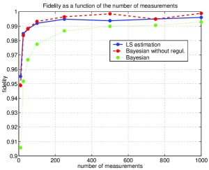
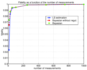
Figure 1: Fidelity as a function of $n$ for a pure state ($s_{pure}$) and a mixed state ($s_{mixed}$)

The result of the Bayesian estimation (dotted line) shows the weakest performance because of the conditioning feature of the method: the conditioned joint probability density function gives worse estimation, than the original one (dashed line). On the other hand, the original Bayesian without conditioning tends to give defective Bloch vector estimates with length greater than one. The price of the validity of the Bayesian method with conditioning is the precision for (near) pure states. It is apparent that the least squares estimation does not have the above problem.

The situation is a little bit different for estimating mixed states (${s_{mixed}}=[0.3,-0.4,\allowbreak 0.3]^{T}$). It can be seen that the two kinds of Bayesian estimation differ only for small $n$’s. When $n$ is greater than $25$, the conditioning has no traceable effect, i.e. the Bayesian estimation with and without conditioning gives the same result. Least squares method also works a little bit better for mixed states than for pure states, at least for larger $n$’s. It can be seen that pure states are a challenge for both methods but least squares handles this difficulty a bit better.

In order to investigate more deeply the behavior of the estimates with low number of measurements we show the variation of the fidelities as a function of the number of measurements in the interval $n=[5,150]$ for both the pure and mixed states above (see Fig. 2).

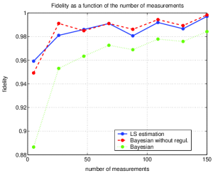
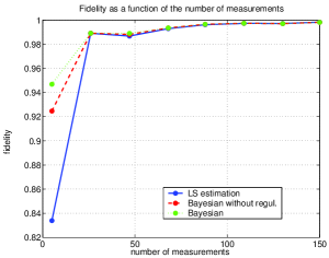
Figure 2: Fidelity as a function of low $n$ for a pure state ($s_{pure}$) and a mixed state ($s_{mixed}$)

It was expected that the Bayesian estimates outperform the LS one for low number of experiments, but it is only true in the case of mixed states. For pure states the overly conservative conditioning of the Bayes method causes a bias. In addition, one can notice, that the effects related to the low number of measurements can be seen only when $n<25$.

Hilbert-Schmidt norm. For Hilbert-Schmidt norm, it was expected to decrease to zero in the limit. The experiments seem to come up to expectations (Fig. 3). In the case of pure states the same phenomena is noticeable as for fidelity.

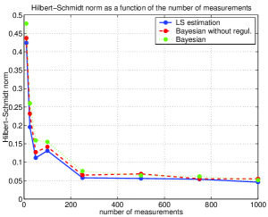
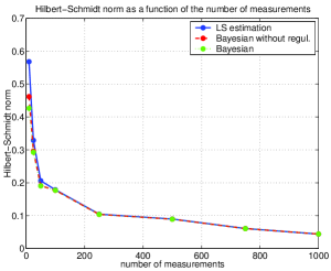
Figure 3: The Hilbert-Schmidt norm as a function of $n$ for a pure state ($s_{pure}$) and a mixed state ($s_{mixed}$)

If one zooms on the low number of measurement region in Fig. 3 then the picture in Fig. 4 results.

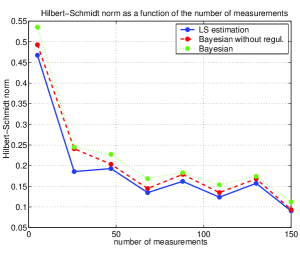
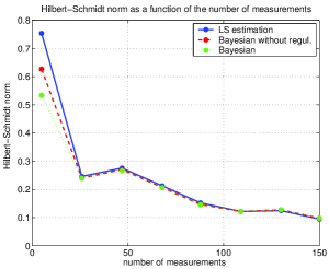
Figure 4: The Hilbert-Schmidt norm as a function of low $n$ for a pure state ($s_{pure}$) and a mixed state ($s_{mixed}$)

Here we can see the same effects as for the fidelity, but in a less exposed way. Thus fidelity seems to be a more sensitive indicator of performance than the Hilbert-Schmidt norm.

Variance. The variance of the estimates were computed for the Bayesian estimation before conditioning. As it was expected, there is no apparent difference between the variance for the three spin components $s_{1},s_{2},$ and $s_{3}$ and the variance decreases with $n$. The fact that the state to be estimated is a pure or a mixed state also does not have any effect on the result (Fig. 5). The same effect can be seen if one focuses on the low number of measurement region, as seen in Fig. 6.

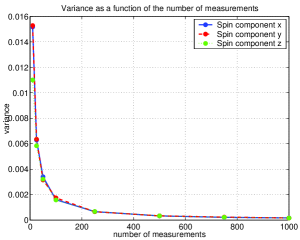
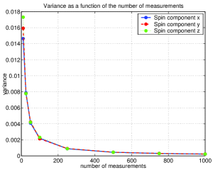
Figure 5: Variance as a function of $n$ for a pure state ($s_{pure}$) and a mixed state ($s_{mixed}$)

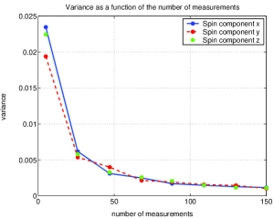
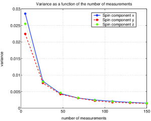
Figure 6: Variance as a function of low $n$ for a pure state ($s_{pure}$) and a mixed state ($s_{mixed}$)

8.2 The length of the Bloch vector

During the second set of experiments the length of the Bloch vector was varying. Its direction was ${s}=[0.5774,\,0.5774,\,0.5774]^{T}$. The expectation to fidelity was to be relatively independent of the Bloch vector length $\|s\|$. The experiment results can be seen in Fig. 7. The first picture shows the case $n=100$, where, in spite of the big variance, the conditioned Bayesian shows an increase near the pure state ($\|s\|=1$). At $n=900$ it is more apparent that LS and conditioned Bayesian methods (both have certain conditioning feature to avoid faulty estimates near $\|s\|=1$, see (18), (14)) have worse performance near pure states. Fig. 8 shows fidelity between $\|s\|=0.9$ and $\|s\|=1$ for $n=900$, where the above mentioned phenomena can be seen more clearly.

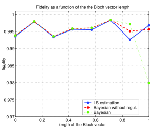
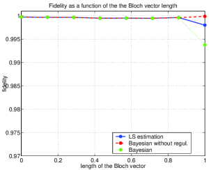
Figure 7: Fidelity as a function of $\|s\|$ for $n=100$ and $n=900$

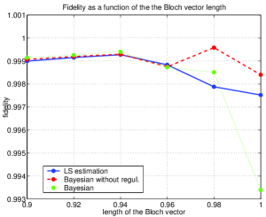
Figure 8: Fidelity as a function of $\|s\|$ for $n=900$

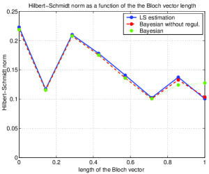
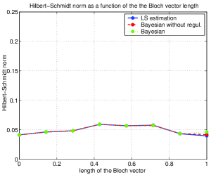
Figure 9: Hilbert-Schmidt norm as a function of $\|s\|$ for $n=100$ and $n=900$

As it was expected, the Hilbert-Schmidt norm seems to be constant for varying Bloch vector lengths, Fig. 9 shows the simulation results. For relatively small $n$ the variance is rather big but increasing the number of measurements it can be seen that the Hilbert-Schmidt norm is almost constant. Near $\|s\|=1$ there is a small increasing for the conditioned Bayesian method.

The expectation for variance was to be independent of Bloch vector length. Fig. 10 shows the results with the same variance-scale as in Fig. 5. The first graph is the results for 100 measurements, the other one is for $n=900$. The result are in accordance with Fig. 5. As it was expected, the two graphs can be regarded as constants.

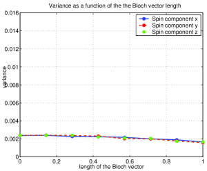
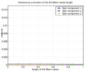
Figure 10: Variance as a function of $\|s\|$ for $n=100$ and $n=900$

9 Conclusion

The performance of two state estimation methods, the Bayesian state estimation as a statistical method and the least squares (LS) method as an optimization-based method is investigated in this paper by using simulation experiments. The fidelity and the Hilbert-Smith norm of the estimation error as well as the empirical variance of the estimate are used as performance indicator quantities. The variation of these quantities as functions of the number of measurements and the length of the Bloch vector are computed.

It is found that fidelity is the best indicator for the quality of an estimate from the investigated three performance indicator quantities from both qualitative and quantitative point of view. For state estimation of a single qubit the region of the ’low measurement number’ being $n<25$ and the ’large measurement number’ $n>200$ has been determined experimentally. As for the comparison of the different state estimation methods we have found that the Bayesian method could outperform the LS estimation only in the case of mixed states for low number of measurements (below $n=25$).

The investigated methods were found to be quite sensitive to the length of the Bloch vector, i.e. to the fact if a pure or mixed state was the one to be estimated. The methods that are not informed about the purity of the state can perform quite badly if they are used to estimate a pure state or a ”nearly pure” state.

It is also found that the way of conditioning is critical for the methods capable of estimating both pure and mixed states. The simple length constraint of the least squares method (in (18)) seems to work quite effectively, thus a version of the Bayesian estimation method with LS-type constraining is a good candidate of an improved stochastic state estimation method.

To handle somehow the difficulties related to estimating nearly pure states one should avoid to use a flat geometry on the state space but one should probably use a suitably defined special Riemannian geometry instead.

References

- [1] F. Albertini and D. D’Alessandro. Model identification for spin networks. Linear Algebra and its Applications, 394:237–256, 2005.
- [2] L.M. Artiles, R. Gill, and M.I. Guta. An invitation to quantum tomography. Journal of the Royal Statistical Society (B), 67:109–134, 2005.
- [3] E. Bagan, M. Baig, R. Munoz-Tapia, and A. Rodriguez. Collective vs local measurements in qubit mixed state estimation. Phys. Rev. A, 61:061307, 2003.
- [4] E. Bagan, M. A. Ballester, R. Munoz-Tapia, and O. Romero-Isart. Measuring the purity of a qubit state: entanglement estimation with fully separable measurements. arXiv, quant-ph/0505083:v1, 2005.
- [5] G. M. D’Ariano, M. G. A. Paris, and M. F. Sacchi. Quantum tomography. Quantum Tomographic Methods, Lect. Notes Phys., 649:7–58, 2004.
- [6] G.M. D’Ariano, L. Maccone, and M.G.A. Paris. Orthogonality relations in quantum tomography. Physics Letters A, 276:25–30, 2000.
- [7] M. Hayashi and K. Matsumoto. Asymptotic performance of optimal state estimation in quantum two level system. arXiv, quant-ph/0411073:v1, 2004.
- [8] C. W. Helstrom. Quantum decision and estimation theory. Academic Press, New York, 1976.
- [9] Z. Hradil, J. Summhammer, and H. Rauch. Quantum tomography as normalization of incompatible observations. Phys. Lett. A, 199:20–24, 1999.
- [10] Mathworks Inc. MATLAB software system, 2001. http://www.mathworks.com/.
- [11] M. Keyl. Quantum state estimation and large deviations. arXiv, quant-ph/0412053:v1, 2004.
- [12] R. L. Kosut, I. Walmsley, and H. Rabitz. Optimal experiment design for quantum state and process tomography and Hamiltonian parameter estimation. arXiv, quant-ph/0411093:v1, 2004.
- [13] R. L. Kosut, I. Walmsley, and H. Rabitz. Identification of quantum systems: Maximum linkelihood and optimal experiment design for state tomography. IFAC World Congress, 1.1:Prague (Czech Republic), 2005.
- [14] M.A. Nielsen and I.L. Chuang. Quantum Computation and Quantum Information. Cambridge University Press, Cambridge, 2000.
- [15] A. Uhlmann. The ”transition probability” in the state space of a *-algebra. Rep. Mathematical Phys, 9:273–279, 1976.
- [16] J. von Neumann. Mathematical Foundations of Quantum Mechanics. Princeton University Press, Princeton, 1957.
- [17] J. Řehaček, B.-G. Englert, and D. Kraszlikowski. Minimal qubit tomography. Physical Review A, 70:052321, 2004.