Preprint SB/F/05-336  

Zeno and Anti Zeno effect for a two level system in a squeezed bath

D.F. Mundarain and J. Stephany

Departamento de Física, Universidad Simón Bolívar,

Apartado 89000, Caracas 1080A, Venezuela.

We discuss the appearance of Zeno (QZE) or anti-Zeno (QAE) effect in an exponentially decaying system. We consider the quantum dynamics of a continuously monitored two level system interacting with a squeezed bath. We find that the behavior of the system depends critically on the way in which the squeezed bath is prepared. For specific choices of the squeezing phase the system shows Zeno or anti-Zeno effect in conditions for which it would decay exponentially if no measurements were done. This result allows for a clear interpretation in terms of the equivalent spin system interacting with a fictitious magnetic field.

 

UNIVERSIDAD SIMÓN BOLÍVAR

1 Introduction

The suppression or modification of the rate of quantum transitions in a system, due to successive measurements is known as the quantum Zeno effect (QZE) [1, 2, 3]. This term has been applied both to the elimination of the induced transitions as in the case of Rabi oscillations on a two level system, or to the reduction of the decay rate on an unstable system. The first situation was experimentally achieved in 1990 [4] and the second one in 2001 [5].

An interesting issue in relation with the QZE is wether it appears or not in exponentially decaying systems. In their article of 1977 Chiu, Sudarshan and Misra [2] show that in general, an unstable system has three decaying regimens. For short time intervals, $t\leq T_{1}$ or very large ones $t\geq T_{2}$, with $T_{1}$ and $T_{2}$ some time scales, the system depart from the exponentially decaying behavior shown for $T_{1}\leq t\leq T_{2}$. They also predict that frequent measurements led to the QZE if the time interval between successive measurements is shorter than $T_{1}$. In the experiment of Ref. [5] for example, for short times, the decay rate of the system is remarkably slower than exponential. This could lead to think that QZE only occurs when the time between measurements is short enough to exploit the departure from the exponential decay law. Nevertheless in a recent article Koshino and Shimizu [6] predicted the appearance of QZE even for systems with an exponential decay law in the case when the detector has a finite window of sensibility. For this case they analyze explicitly the interaction between the quantum system and the detector and interpreted the changes induced by the interaction as the effect of the measurement. They refer [7] to this analysis as the dynamical formalism as opposed to the conventional formalism where the measurements are taken as projections consistent with the quantum collapse postulate of von Neumann.

For a closed system the theoretical description of the measurement in terms of the projection postulate predicts a complete Zeno effect, that is the freezing of the quantum system in the initial state. For such system with a hamiltonian ${\it H}$, the evolution is determined by the Schrödinger equation

$$\frac{\partial}{\partial t}|\psi(t)\rangle=\frac{1}{i\hbar}{\it H}|\psi(t)\rangle$$ (1)

If the observable ${\it A}$ to be measured has eigenvalues $a_{m}$ and supposing that at $t=0$ the system is in the eigenstate $|a_{n}\rangle$, the probability of obtaining the result $a_{n}$ for a short time interval $\Delta t\geq 0$ is given by,

$$P_{n}(\Delta t)=\left(1-\frac{\Delta t^{2}}{\hbar^{2}}\Delta_{n}^{2}{\it H}\right)$$ (2)

where

$$\Delta_{n}^{2}{\it H}=\langle a_{n}|{\it H}^{2}|a_{n}\rangle-\langle a_{n}|{\it H}|a_{n}\rangle^{2}$$ (3)

If one considers $S$ successive projective measurements separated by the same interval $\Delta t$ the probability of obtaining in each case the same result $a_{n}$ is:

$$P_{n}(S,\Delta t)=\left(1-\frac{\Delta t^{2}}{\hbar^{2}}\Delta_{n}^{2}{\it H}\right)^{S}$$ (4)

In the limit of very frequent measurements [8], that is when $S>>1,\ \ \ \ S\Delta t\rightarrow t$ the probability of measuring $a_{n}$ every time is

$$P_{n}^{(cm)}(t)=\lim_{S\rightarrow\infty}P_{n}(S,t/S)=\lim_{S\rightarrow\infty}\left(1-\frac{t^{2}}{S^{2}\hbar^{2}}\Delta_{n}^{2}{\it H}\right)^{S}=1$$ (5)

which corresponds to a complete Zeno effect.

For open systems in contact with the environment some limitations affect the appearance of the QZE even if projective measurements are being done. For time intervals which are greater than the correlation time of the bath, the evolution may be described in terms of the density matrix by a master equation of the Liouville type,

$$\frac{\partial\rho}{\partial t}={\it L}\left\{\rho\right\}.$$ (6)

with ${\it L}\left\{\rho\right\}$ some appropriate operator depending on $\rho$. Then, for a short time interval $\Delta t$, the density operator is given in terms of its initial value by

$$\rho(\Delta t)=\rho(0)+{\it L}\left\{\rho(0)\right\}\Delta t$$ (7)

If the initial state is $\rho(0)=|a_{n}\rangle\langle a_{n}|$ the probability of measuring $a_{n}$ in $S$ consecutive measurements separated by time intervals $\Delta t$ is,

$$P_{n}(S,\Delta t)=(1+\langle a_{n}|{\it L}\left\{\rho(0)\right\}|a_{n}\rangle\Delta t)^{S}\simeq(\exp\left\{\langle a_{n}|{\it L}\left\{\rho(0)\right\}|a_{n}\rangle\ \Delta t\right\})^{S}$$ (8)

In the limit $S>>1,\ \ \ \ S\Delta t\rightarrow t$, of very frequent measurements one obtains,

$$P_{n}^{(cm)}(t)=\exp\left\{\langle a_{n}|{\it L}\left\{\rho(0)\right\}|a_{n}\rangle\ \ t\right\}$$ (9)

Here the freezing of the initial condition for continuous measurements is achieved only if

$$\langle a_{n}|{\it L}\left\{\rho(0)\right\}|a_{n}\rangle=0$$

This illustrates the fact that in general, both the the intrinsical properties of the system and the characteristics of the measurement affect the possibility of displaying the quantum Zeno effect.

A related issue that we have to consider comes from the observation that for an unstable quantum system the probability of obtaining a specific result in a measurement may increase, decrease or even oscillate in time as the result of its undisturbed evolution. Decay rates may also be affected by measurements done at particular instants of time, an effect which has in principle nothing to do with the QZE. This suggests that the interaction of the system with a non trivial electromagnetic bath may modify the decay rates even for an exponentially decaying system. In this paper we show that such mechanism can be actually used to induce QZE or QAE in a two level system. For this system interacting with a squeezed bath QZE or QAE may appear when measuring the fictitious spin along a specific direction depending on the relative phase of the squeezing and the chosen direction. This may be interpreted as an effect of the orientation induced on the fictitious spin by the fictitious magnetic field defined by the quadratic fluctuations of the true electromagnetic field.

2 The two level system in a squeezed bath

In the rotating wave approximation the hamiltonian which better describes the atom-field interaction has the following structure, [9, 10]:

$${\it H}=\sum_{\bf k}\hbar\nu_{k}a_{\bf k}^{\dagger}a_{\bf k}+\frac{1}{2}\hbar\omega\sigma_{z}+\hbar\sum_{\bf k}g_{\bf k}\left(\sigma_{+}a_{\bf k}+a_{\bf k}^{\dagger}\sigma_{-}\right)$$ (10)

where $g_{\bf k}$ are the atom-field couplings constants, $a_{\bf k}$ and $a_{\bf k}^{\dagger}$ are the creation and annihilation operators of the multimodal field and $\sigma_{+}$ and $\sigma_{-}$ are the ladder operators

$$\sigma_{+}=\left(\begin{array}[]{cc}0&1\\ 0&0\end{array}\right)\qquad\sigma_{-}=\left(\begin{array}[]{cc}0&0\\ 1&0\end{array}\right)\ \ ,$$ (11)

with $\sigma_{x}$, $\sigma_{y}$ and $\sigma_{z}$ are the Pauli matrices,

$$\sigma_{x}=\left(\begin{array}[]{cc}0&1\\ 1&0\end{array}\right)\qquad\sigma_{y}=\left(\begin{array}[]{cc}0&-i\\ i&0\end{array}\right)\qquad\sigma_{z}=\left(\begin{array}[]{cc}1&0\\ 0&-1\end{array}\right)\ \ .$$ (12)

If the field is prepared in a broadband squeezed vacuum state characterized by $\xi=re^{i\phi}$ it was demonstrated that, [9, 10]:

$$\langle a_{\bf k}\rangle=\langle a_{\bf k}^{\dagger}\rangle=0$$

$$\langle a_{\bf k}^{\dagger}a_{\bf k^{\prime}}\rangle\delta_{\bf kk^{\prime}}=N\delta_{\bf kk^{\prime}}$$

$$\langle a_{\bf k}a_{\bf k^{\prime}}^{\dagger}\rangle=\delta_{\bf kk^{\prime}}=(N+1)\delta_{\bf kk^{\prime}}$$

$$\langle a_{\bf k}a_{\bf k^{\prime}}\rangle=-e^{i\phi}\cosh(r)\sinh(r)\delta_{\bf k^{\prime},2k_{0}-k}=e^{i\phi}M\delta_{\bf k^{\prime},2k_{0}-k}$$

$$\langle a_{\bf k}^{\dagger}a_{\bf k^{\prime}}^{\dagger}\rangle=-e^{-i\phi}\cosh(r)\sinh(r)\delta_{\bf k^{\prime},2k_{0}-k}=e^{-i\phi}M\delta_{\bf k^{\prime},2k_{0}-k}\ \ ,$$ (13)

where $N=\sinh^{2}(r)$, $M=\sqrt{N(N+1)}$. Here ${\bf k_{0}}$ is the wave number associated to the resonant frequency of the squeezing device. In the interaction picture the master equation for this system takes the form of Eq. (6) with,

$$L\{\rho\}= \frac{1}{2}\gamma\left(N+1\right)\left(2\sigma_{-}{\rho}\sigma_{+}-\sigma_{+}\sigma_{-}{\rho}-{\rho}\sigma_{+}\sigma_{-}\right)$$ (14)

$$\frac{1}{2}\gamma N\left(2\sigma_{+}{\rho}\sigma_{-}-\sigma_{-}\sigma_{+}{\rho}-{\rho}\sigma_{-}\sigma_{+}\right)$$

$$-\gamma Me^{i\phi}\sigma_{+}{\rho}\sigma_{+}-\gamma Me^{-i\phi}\sigma_{-}{\rho}\sigma_{-}\ \ .$$

Here $\gamma$ is the decay constant of the system in the vacuum. This equation may be rewritten using Bloch’s representation for the two level system density matrix in the form,

$$\rho=\frac{1}{2}\left(1+\rho_{x}\sigma_{x}+\rho_{y}\sigma_{y}+\rho_{z}\sigma_{z}\right)\ \ .$$ (15)

Using Eqs. (14,15), the master equation (6) takes the form,

$$\frac{\partial\rho}{\partial t}= -\frac{1}{2}\gamma\left(N+1\right)\left((1+\rho_{z})\sigma_{z}+\frac{1}{2}\rho_{x}\sigma_{x}+\frac{1}{2}{\rho_{y}}\sigma_{y}\right)$$ (16)

$$+\frac{1}{2}\gamma N\left((1-\rho_{z})\sigma_{z}-\frac{1}{2}\rho_{x}\sigma_{x}-\frac{1}{2}{\rho_{y}}\sigma_{y}\right)$$

$$-\frac{1}{2}\gamma M\rho_{x}(\cos(\phi)\sigma_{x}-\sin(\phi)\sigma_{y})$$

$$+\frac{1}{2}\gamma M\rho_{y}(\sin(\phi)\sigma_{x}+\cos(\phi)\sigma_{y})$$

This is equivalent to the following differential equations for $(\rho_{x},\rho_{y},\rho_{z})$:

$$\dot{\rho_{x}}=-\gamma\left(N+1/2+M\cos(\phi)\right)\rho_{x}+\gamma M\sin(\phi)\rho_{y}$$

$$\dot{\rho_{y}}=-\gamma\left(N+1/2-M\cos(\phi)\right)\rho_{y}+\gamma M\sin(\phi)\rho_{x}$$

$$\dot{\rho_{z}}=-\gamma\left(2N+1/2\right)\rho_{z}-\gamma$$ (17)

The solutions of these equations are given by,

$$\rho_{x}(t)= \left(\rho_{x}(0)\sin^{2}(\phi/2)+\rho_{y}(0)\sin(\phi/2)\cos(\phi/2)\right)e^{-\gamma(N+1/2-M)\,t}$$ (18)

$$+\left(\rho_{x}(0)\cos^{2}(\phi/2)-\rho_{y}(0)\sin(\phi/2)\cos(\phi/2)\right)e^{-\gamma(N+1/2+M)\,t}$$

$$\rho_{y}(t)= \left(\rho_{y}(0)\cos^{2}(\phi/2)+\rho_{x}(0)\sin(\phi/2)\cos(\phi/2)\right)e^{-\gamma(N+1/2-M)\,t}$$ (19)

$$+\left(\rho_{y}(0)\sin^{2}(\phi/2)-\rho_{x}(0)\sin(\phi/2)\cos(\phi/2)\right)e^{-\gamma(N+1/2+M)\,t}$$

$$\rho_{z}(t)=\rho_{z}(0)e^{-\gamma(2N+1)t}+\frac{1}{2N+1}\left(e^{-\gamma(2N+1)t}-1\right)$$ (20)

From these expressions one can read the dependence of the decay rates of the system on the phase $\phi$ of the squeezing. In particular, for $\phi=0$, $\phi=\pi$ or for the critical angles $\phi_{z}=2\arctan(-\rho_{y}(0)/\rho_{x}(0))$ or $\phi_{AZ}=2\arctan(\rho_{x}(0)/\rho_{y}(0))$, the system has a purely exponential behavior with the decay rates presented in Table 1.

$\rho_{x}(t)/\rho_{x}(0)$ $\rho_{y}(t)/\rho_{y}(0)$ $\phi=0\quad$ $e^{-\gamma(N+1/2+M)t}$ $e^{-\gamma(N+1/2-M)t}$ $\phi=\pi\quad$ $e^{-\gamma(N+1/2-M)t}$ $e^{-\gamma(N+1/2+M)t}$ $\phi=\arctan\left(-\frac{\rho_{y}(0)}{\rho_{x}(0)}\right)$ $e^{-\gamma(N+1/2+M)t}$ $e^{-\gamma(N+1/2+M)t}$ $\phi=\arctan\left(\frac{\rho_{x}(0)}{\rho_{y}(0)}\right)$ $e^{-\gamma(N+1/2-M)t}$ $e^{-\gamma(N+1/2-M)t}$

Table 1: Decay rates for critical angles

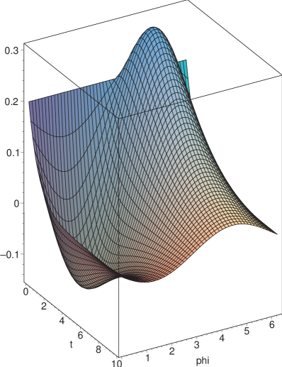
Figure 1: $\rho_{x}(t,\phi)$, $\rho_{x}(0)=0.2$ , $\rho_{y}(0)=-\sqrt{1-\rho_{x}(0)^{2}}$, $\rho_{z}(0)=0$, $N=1$, $\gamma=1$

In Fig.(1) we show the dependence of $\rho_{x}(t)=\langle\sigma_{x}\rangle$ with the phase as given by Eq. (18). In particular the exponential decay for the preferred values of the phase may be observed.

3 The origin of the critical angles

Before discussing the effect of the measurements in the evolution of the two level system let us first explore the properties of the fictitious magnetic field associated to the squeezed state in order to justify the decay rates for the two critical angles appearing in Table 1.

Consider the atomic part of the Hamiltonian (10). In terms of the Pauli matrices it takes the form,

$${\it H}_{Atomic}=\frac{1}{2}\hbar\omega\sigma_{z}+\frac{1}{2}\hbar\sigma_{x}\sum_{\bf k}g_{\bf k}\left(a_{\bf k}+a_{\bf k}^{\dagger}\right)+\frac{1}{2}\hbar\sigma_{y}\sum_{\bf k}ig_{\bf k}\left(a_{\bf k}-a_{\bf k}^{\dagger}\right)\ .$$ (21)

This can be rewritten in the form

$${\it H}_{Atomic}=-\gamma_{0}\,{\bf B\cdot S}\ \ .$$ (22)

where $\gamma_{0}$ is an arbitrary constant with dimensions of charge divided by mass, ${\bf S}$ is the fictitious spin associated to the two level system and ${\bf B}$ is the quantum fictitious magnetic field with components,

$$B_{x}=-\frac{1}{\gamma_{0}}\sum_{\bf k}g_{\bf k}\left(a_{\bf k}+a_{\bf k}^{\dagger}\right)$$ (23)

$$B_{y}=-\frac{1}{\gamma_{0}}\sum_{\bf k}ig_{\bf k}\left(a_{\bf k}-a_{\bf k}^{\dagger}\right)$$ (24)

$$B_{z}=-\frac{\omega}{\gamma_{0}}\ \ .$$ (25)

Clearly $<B_{x}>=0$ and $<B_{y}>=0$. For the quadratic fluctuations the result is,

$$<B_{x}^{2}> = \frac{\Gamma}{4}\left(\sinh^{2}(r)+\cosh^{2}(r)-2\cos(\theta)\sinh(r)\cosh(r)\right)$$

$$= \Gamma\left(N+\frac{1}{2}-M\cos(\phi)\right)$$

$$<B_{y}^{2}> = \frac{\Gamma}{4}\left(\sinh^{2}(r)+\cosh^{2}(r)+2\cos(\theta)\sinh(r)\cosh(r)\right)$$

$$= \Gamma\left(N+\frac{1}{2}+M\cos(\phi)\right)$$

where

$$\Gamma=\frac{1}{2\gamma_{0}^{2}}\sum_{\bf k}|g_{\bf k}|^{2}.$$

Here $\Gamma=\sum_{k}|g_{k}|^{2}$ is taken to be finite, which means that only a finite subset of the modes in the bath is coupled effectively to the system. For $<B^{2}>$ we have,

$$<B^{2}>=\frac{\Gamma}{2}\left(\sinh^{2}(r)+\cosh^{2}(r)\right)=\frac{\Gamma}{2}\left(2N+1\right),$$ (28)

which does not depend on $\phi$.

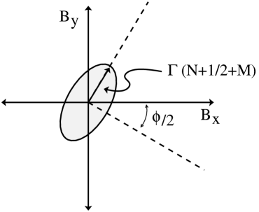
Figure 2: Fluctuations of the fictitious magnetic field.

These fluctuations may be represented in phase space as an ellipse whose axis are rotated by an angle $\phi/2$. As is illustrated in Fig. (2), the semi-axis have magnitudes $\Gamma\left(N+1/2+M\right)$ and $\Gamma\left(N+1/2-M\right)$.

Comparing with the results of the previous section, we can observe, that for zero phase the decay rate for $\rho_{x}=\langle\sigma_{x}\rangle$ is proportional to the fluctuations of the fictitious magnetic field component $B_{y}$ and the decay rate for $\rho_{y}=\langle\sigma_{y}\rangle$ is proportional to the fluctuations of $B_{x}$. Also, the decay rate for $\rho_{z}$ is proportional to $<B^{2}>$. In general, for other values of the phase, the component $(\rho_{x},\rho_{y})$ of Bloch’s vector orthogonal to the major semi-axis of the phase space ellipse used to represent the magnetic field fluctuations, has a decay rate proportional to $\Gamma\left(N+1/2+M\right)$ and the component orthogonal to the minor semi-axis has a decay rate proportional to $\Gamma\left(N+1/2-M\right)$. The phase $\phi_{Z}=2\arctan\left(-\rho_{y}(0)/\rho_{x}(0)\right)$ defines a critical value which corresponds to the case when initially the Bloch vector is orthogonal to the major semi-axis. For this value $\rho_{x}$ and $\rho_{y}$ decay with the maximum rate. The complementary case occurs for $\phi_{AZ}=2\arctan(\rho_{x}(0)/\rho_{y}(0))$ in which case $\rho_{x}$ and $\rho_{y}$ decay with the minimum allowed value of the decay rate.

The fact that the decay rates for $\rho_{x}$ and $\rho_{y}$ coincides in both cases is a consequence of the coupled dynamics of these two variables. But if one measures $\sigma_{x}$, the dynamics disentangles and one would expect that the decay rate for $\rho_{x}$ results proportional to the fluctuations of $B_{y}$ only , as in the cases $\phi=0$ or $\phi=\pi$ when there is no coupling at all. Then, we expect the Zeno effect to occur for $\phi_{Z}$ and the anti-Zeno effect to occur for $\phi_{AZ}$ due to the factor $\cos(\phi)$ that appears in the fluctuation of $B_{y}$.

4 Zeno and anti-Zeno effect

Let us now consider explicitly the effect of repeated measurements of the observable $\sigma_{x}$ in the evolution of the system prepared in a state defined by the initial values of $(\rho_{x}(0),\rho_{y}(0),\rho_{z}(0))$. We suppose that the time interval between measurements is very short, but still much greater than the correlation time of the squeezed bath [11]. Then we may describe the evolution of the system by means of a master equation of the form (6). In our analysis we take in fact the correlation time of the squeezed bath to be zero which corresponds to broadband squeezing. For considerations on the finite bandwidth effects se Ref. [11, 12, 13]. On the experimental side squeezing with a bandwidth of up to 1GHz has been reported [14, 15, 16].

The probability that in a very large succession of measurements, the result obtained in all of them is the eigenvalue $+1$ associated to the eigenstate $|+\rangle_{x}$ is given by,

$$P_{+}^{(cm)}(t)=\frac{(1+\rho_{x}(0))}{2}\exp\left\{{}_{x}\langle+|{\it L}\left\{\rho_{1}\right\}|+\rangle_{x}t\right\}$$ (29)

where $\rho_{1}$ is the collapsed density matrix after the measurements and is given by

$$\rho_{1}=|+\rangle_{x\,x}\langle+|\ \ \ ,\ \ \ |+\rangle_{x}=\frac{1}{\sqrt{2}}\left(|+\rangle+|-\rangle\right).$$ (30)

The probability of Eq. (29) is obtained by multiplying the probability corresponding to the first measurement and the probability obtained in Eq. (9) which is valid for the following measurements. If the system is initially in the state $|+\rangle_{x}$ then $\rho_{x}(0)=1$, $\rho_{y}(0)=0$ and $\rho_{z}(0)=0$, in which case Eq. (29) is a particular case of Eq. (9).

One can show that for the squeezed bath,

$${}_{x}\langle+|{\it L}\left\{\rho_{1}\right\}|+\rangle_{x}=-\frac{\gamma}{2}\left(N+\frac{1}{2}+M\cos(\phi)\right).$$ (31)

In this case Eq. (29) reduces to,

$$P_{+}^{(cm)}(t,\phi)=\frac{(1+\rho_{x}(0))}{2}\exp\left\{-\frac{\gamma}{2}\left(N+\frac{1}{2}+M\cos(\phi)\right)t\right\}$$ (32)

We should compare this expression with the probability of measuring the eigenvalue $+1$ by performing an unique measurement at time $t$

$$P_{+}(t,\phi)=\frac{(1+\rho_{x}(t))}{2}.$$ (33)

In Fig.(3) we show that the probability $P_{+}(t,\phi=0)$ decays exponentially to the value $1/2$, that is, for $t\rightarrow\infty$ we have the same probability to measure any of the two eigenvalues. On the other hand the probability $P_{+}^{(cm)}(t,\phi=0)$, i.e the probability to obtain the same value $+1$ in all the measurements, decays exponentially to zero. In the same figure we can see that the probability $P_{+}^{(cm)}(t,\phi=0)$ is smaller than the probability $P_{+}(t,\phi=0)$ for all $t$. Note that, the probability of obtaining the result $+1$ in the last measurement independently of the previous results is of course greater than the probability of obtaining the value $+1$ in all the measurements. Furthermore, if the evolution of the observable $\sigma_{x}$ is not affected by the measurements, the probability to obtain $+1$ in the last measurement independently of the results of the previous measurements is equal to the probability to obtain $+1$ at time $t$ if no other measurement has been done previously. The result shown in Fig.(3) suggest that in fact for $\phi=0$ the evolution of the observable $\sigma_{x}$ is not affected by the measurements.

Changing the phase it is possible to obtain a completely different result. In Fig (4) we show that there exists a time interval for which $P_{+}^{(cm)}(t,\phi_{Z})$ is greater than the $P_{+}(t,\phi_{Z})$. The natural explanation for this, comes from the fact that in this case the measurements do modify the dynamics of the observable.

To study quantitatively this effect it is necessary to work out the changes in the master equation related to the continuous monitoring. If we have the system described by $\rho$ and perform measurements of $\sigma_{x}$ the new density matrix is given by,

$$\rho^{\prime}=P\rho P+(1-P)\rho(1-P)$$ (34)

where $P=|+\rangle_{xx}\langle+|$ is the projector to the eigenvector of $\sigma_{x}$ with eigenvalue $+1$ and $(1-P)$ is the projector to the eigenvector of $\sigma_{x}$ with eigenvalue $-1$.

Between consecutive measurements the free evolution is determined by the free master equation. By considering the free master equation and the collapse in the same expression, it is shown that after the first measurement the master equation with continuous measurements takes the form,

$$\frac{\partial\rho}{\partial t}=P{\it L}(\rho)P+(1-P){\it L}(\rho)(1-P)$$ (35)

Let us now focus in the mean value of the measured observable $\langle\sigma_{x}\rangle=\rho_{x}(t)$. The corresponding probabilities may be computed using Eq. (33). In terms of Bloch’s vector, the master equation with continuous measurements for the two level system in the squeezed bath is given by the following equations,

$$\dot{\rho_{x}} = -\gamma(N+1/2+M\cos(\phi))\rho_{x}+\gamma M\sin(\phi)\rho_{y}$$

$$\dot{\rho_{y}} = 0$$

$$\dot{\rho_{z}} = 0$$ (36)

Since after the first measurement the values of $\rho_{y}$ and $\rho_{z}$ collapse to zero, the solutions for this system are given by ,

$$\rho_{x}(t)=\rho_{x}(0)\exp(-\gamma(N+1/2+M\cos(\phi))t)$$ (37)

$$\rho_{y}(t)=0\qquad\rho_{z}(t)=0.$$ (38)

As we can see from Eq. (37) in presence of very frequent measurements the decay rate of $\rho_{x}$ is proportional to the quantum fluctuation of $B_{y}$.

In Fig. (5), it can be shown the evolution of $<\sigma_{x}>$ for $\phi=0$ with measurements and without measurements. We observe that the evolution is not affected by the measurements. This agrees with the usual assumption that for an unstable system with exponential decay Zeno effect is not observable. In Fig. (6) for $\phi=\phi_{Z}$, one can appreciate the reduction of the decay rate when comparing with the not disturbed case. For the phase $\phi=\phi_{AZ}$ the rate of decaying grows and we have Anti-Zeno effect.

5 Indirect measurements

When indirect measurements are being done, the master equation with continuous monitoring of $\sigma_{x}$ takes the form [8],

$$\frac{\partial\rho}{\partial t}={\it L}(\rho)-\frac{1}{T_{0}}[\,\sigma_{x}\,,\,[\sigma_{x},\rho]\,]$$ (39)

where $T_{0}$ is the coupling constant between the measuring apparatus and the system. Writing this equation in terms of Bloch‘s vector for the two level system in a squeezed bath we have,

$$\dot{\rho_{x}}=-\gamma\left(N+1/2+M\cos(\phi)\right)\rho_{x}+\gamma M\sin(\phi)\rho_{y}$$

$$\dot{\rho_{y}}=-\gamma\left(N+1/2-M\cos(\phi)\right)\rho_{y}+\gamma M\sin(\phi)\rho_{x}-\frac{4}{T_{0}}\rho_{y}$$

$$\dot{\rho_{z}}=-\gamma\left(2N+1/2\right)\rho_{z}-\gamma-\frac{4}{T_{0}}\rho_{z}$$ (40)

The limit $T_{0}\rightarrow\infty$ corresponds to no measurement being done. For $T_{0}\rightarrow 0$ equations (40) transform into equations (36). Then, for these kind of measurements one obtains similar effects that those observed in the previous section for the projective measurements.

6 Conclusion

We have presented an explicit example of a system where the appearance of Zeno (or anti-Zeno) effect may be induced in a regime for which it would decay exponentially if no measurements were done. Working with a two level system in squeezed electromagnetic bath, we found that these effects may be induced by choosing adequately the phase of the squeezing of the bath. This result is interpreted as the natural result of the interaction of the equivalent spin system with the fluctuating fictitious magnetic field.

7 Acknowledgments

This work was supported by Did-Usb grant Gid-30 and by Fonacit grant G-2001000712.

Figure 3: Solid line: $P_{+}(t)$. Dashed line: $P_{+}^{(cm)}(t,\phi=0)$. $\rho_{x}(0)=0.5$, $\rho_{y}(0)=-\sqrt{1-\rho_{x}(0)^{2}}$, $\rho_{z}(0)=0$, $N=1$, $\gamma=1$

Figure 4: Solid line: $P_{+}(t)$. Dashed line: $P_{+}^{(cm)}(t,\phi_{Z})$. $\rho_{x}(0)=0.5$, $\rho_{y}(0)=-\sqrt{1-\rho_{x}(0)^{2}}$, $\rho_{z}(0)=0$, $N=1$, $\gamma=1$

Figure 5: Solid line: $\rho_{x}(t)$ undisturbed. Dashed line: $\rho_{x}(t)$ with measurements. $\rho_{x}(0)=0.5$, $\rho_{y}(0)=-\sqrt{1-\rho_{x}(0)^{2}}$, $\rho_{z}(0)=0$, $\phi=0$, $N=1$, $\gamma=1$

Figure 6: Solid line: $\rho_{x}(t)$ undisturbed. Dashed line: $\rho_{x}(t)$ with measurements. $\rho_{x}(0)=0.5$, $\rho_{y}(0)=-\sqrt{1-\rho_{x}(0)^{2}}$, $\rho_{z}(0)=0$, $\phi=\phi_{Z}$, $N=1$, $\gamma=1$

Figure 7: Solid line: $\rho_{x}(t)$ undisturbed. Dashed line: $\rho_{x}(t)$ with measurements. $\rho_{x}(0)=0.5$, $\rho_{y}(0)=-\sqrt{1-\rho_{x}(0)^{2}}$, $\rho_{z}(0)=0$, $\phi=\phi_{AZ}$, $N=1$, $\gamma=1$

References

• [1] B. Misra and E. C. Sudarshan, J.Math.Phys. 18, 756 (1977).
• [2] C. B. Chiu, E. C. Sudarshan and B. Misra, Phys. Rev D 16, 520 (1977).
• [3] A. Peres, Am.J.Phys 48, 931 (1980).
• [4] W. M. Itano, D. J. Heinzen, J. J. Bollinger and D. J. Wineland, Phys. Rev. A 41, 2295 (1990).
• [5] M. C. Fischer, B. Gutierrez-Medina and M. G. Raizen, Phys. Rev. Lett 87, 040402 (2001).
• [6] K. Koshino and A. Shimizu, Phys. Rev. Lett. 92, 30401 (2004).
• [7] K. Koshino, Phys. Rev. A 71, 034104 (2005).
• [8] V. B. Braginsky and F.Y. Khalili, Quantum Measurement, Cambridge University Press, 1992.
• [9] C. W. Gardiner, Phys. Rev. Lett. 56, 1917 (1986)
• [10] M. O. Scully and M. Suhail Zubairy, Quantum Optics. Cambridge University Press (1997).
• [11] C. W. Gardiner, A. S. Parkins and M. J. Collett, J.Opt. Soc. Am B4, 1683 (1987).
• [12] A. S. Parkins and C. W. Gardiner, Phys Rev A37, 3867 (1988).
• [13] R.Tanas and T.El-Shahat, Acta.Phys.Slov. 48, 301 (1998).
• [14] D. D. Crouch, Phys Rev A38, 508 (1988).
• [15] S. Machida and Y. Yamamoto, Phys. Rev. Lett 60, 792 (1988).
• [16] T. Hirano, K. Kotani, T. Ishibashi, S. Okude and T. Kuwamoto, Opt. Lett. 30, 1722 (2005).
Refer to caption