Controlled and combined remote implementations
of partially unknown quantum operations of multiqubits
using GHZ states

Abstract

We propose and prove protocols of controlled and combined remote implementations of partially unknown quantum operations belonging to the restricted sets [An Min Wang: PRA, 74, 032317(2006)] using GHZ states. We detailedly describe the protocols in the cases of one qubit, respectively, with one controller and with two senders. Then we extend the protocols to the cases of multiqubits with many controllers and two senders. Because our protocols have to demand the controller(s)’s startup and authorization or two senders together working and cooperations, the controlled and combined remote implementations of quantum operations definitely can enhance the security of remote quantum information processing and potentially have more applications. Moreover, our protocol with two senders is helpful to farthest arrive at the power of remote implementations of quantum operations in theory since the different senders perhaps have different operational resources and different operational rights in practice.

I Introduction

Quantum teleportation Bennett is one of the most striking developments in quantum theory. It indicates that a quantum state can be remotely transferred in a completely different way compared with a classical state. Thus, one would like to know whether and how a quantum operation can also be remotely transferred in a completely different way compared with a classical operation. This problem is just so-called the remote implementation of quantum operation (RIO), which was ever studied successfully by Huelga, Plenio and Vaccaro (HPV) Huelga1 ; Huelga2 for the case of one qubit. Recently, we proposed and proved a protocol of remote implementations of partially unknown quantum operations of multiqubits via deducing the general restricted sets and finding the unified recovery operations MyRIO .

Remote implementation of a quantum operation means that this quantum operation performed on a local system (sneder’s) is teleported and it acts on an unknown state belonging to a remote system (receiver’s) Huelga1 ; Huelga2 ; MyRIO . Here, a sender is a person who transfers a quantum operation, and a receiver is a person whose system receives this quantum operation and this quantum operation acts on an unknown state belonging to him/her. Obviously, the RIO is different from simple teleportation of quantum operation without action, and it is also not an implementation of nonlocal quantum operation Cirac ; Eisert , although there are the closed connections among them. Actually, all of them play the important roles in distributed quantum computation Cirac ; Eisert , quantum program Nielsen ; Sorensen and the other remote quantum information processing tasks. Recently, a series of works on the remote implementations of quantum operations appeared and made some interesting progress both in theory Collins ; Huelga1 ; Huelga2 ; MyRIO and in experiment Huang ; Xiang ; Huelga3 .

Both HPV’s and our recent protocols use Bell states as a quantum channel. However, it is well-known that GHZ states GHZ are also very important quantum resource in quantum information processing and communication (QIPC). Just motivated by the scheme of teleportation of quantum states using GHZ state Karlsson ; Yang ; Deng and the fact that it has been successfully applied to quantum secret sharing Hillery , we would like to investigate the remote implementations of quantum operations using GHZ state(s). Nevertheless, the more important motivations using state(s)in our protocols are to enhance security, increase variety, extend applications as well as advance efficiency via fetching in some controllers and two senders. Our results again indicate that GHZ states are powerful resources in QIPC.

It is useful and interesting to investigate the remote implementations of partially unknown quantum operations because they will consume less overall resource than one of the completely unknown quantum operations, and such RIOs can satisfy the requirements of some practical applications. Here, the “partially unknown” quantum operations are thought of as those belonging to some restricted sets which satisfy some given restricted conditions. In Refs. Huelga1 ; Huelga2 ; MyRIO , the restricted sets of quantum operations were seen to be still a very large set of unitary transformations because their unknown elements take continuous values. In the simplest case of one qubit, two kinds of restricted sets of quantum operations are, respectively, a set of diagonal operations and a set of antidiagonal operations Huelga2 . For the cases of multiqubits, we obtained the general forms of restricted sets of quantum operations and the unified recovery operations, then proposed and proved our protocol of remote implementations of quantum operations belonging to the restricted sets in our recent work MyRIO . Specially, our restricted sets of quantum operations are not reducible to a direct product of two restricted sets of one-qubit operations, our recovery operations have general and unified forms, and so our protocol can be thought of as a development of HPV protocol to multiqubits systems but not a simple extension of HPV protocol Huelga2 .

It must be emphasized that the main advantage using GHZ states in the RIO protocols is to provide ability for fetching in (many) controller(s) or/and more than one sender. When there is(are) the controller(s), we call the remote implementation of quantum operations as controlled one, when there are more than one sender, we called the remote implementation of quantum operations as combined one. A controlled remote implementation of quantum operation has to have the controllers’ participation. A combined remote implementation of quantum operations has to have the senders’ cooperation. Otherwise, the RIOs cannot be faithfully and determinedly completed.

In the controlled RIOs, not only a controller plays such a role that the quantum channel between sender and receiver is opened by his/her operations, but also the controller’s measurement (classical information) impacts the form of the sender’s operations or the receiver’s operation. This implies that the controller’s action contains “start up” and “authorization” so that the RIOs can be faithfully and determinedly completed. Just based on this fact, we can say the controlled RIOs definitely enhance the security of remote quantum information communication and processing. In addition, varying with the ways of authorization by the controller, the steps in RIO protocols have their different forms. It seems to bring about some complicated expressions of our protocols, but aiming at the different cases, the controlling process needs such variety. For example, if the controller trusts in the sender or is easy to communicate with the sender, he/she authorizes to the sender; if the controller trusts in the receiver or is easy to communicate with the receiver he/she authorizes to the receiver; if the controller hopes to keep the “say last words”, he/she authorizes to the receiver at a chosen stage of the protocols.

While in the combined RIOs, the later sender has to obtain the classical information from the former one by one in the sending sequence of protocols so that he/she can correctly choose his/her operation. Therefore, the combined RIOs can also definitely enhance the security of remote quantum information communication and processing. Note that the security enhancement is in classical sense, this can be called so-called “sequential multiple-safety”. This concept can be understood and illustrated by a classical example of opening safe-deposit box. For simplicity, let us only consider the case of sequential double-safety. This example is how to open a safe-deposit box with two locks and its every lock has a set of various keys. Suppose the set of keys of the first lock are $k_{1}^{A},k_{1}^{B},\cdots$, the set of keys of the second lock are $k_{2}^{A},k_{2}^{B},\cdots$. Opening the safe-deposit box needs to use the sequential and paired keys $(k_{1}^{A},k_{2}^{A})$, or $(k_{1}^{B},k_{2}^{B}),\cdots$ to complete it. Otherwise the safe-deposit box can not be opened. In other words, two guardians (corresponding two senders) have to cooperate each other. When the first guardian opens the first lock using some given key $k_{1}^{C}$ (corresponding a quantum operation belonging to some given restricted set), he/she has to tell the second guardian his/her using $C$ key so that the second guardian can correctly use $k_{2}^{C}$ to open the safe-deposit box. Of course, we can say that the combined RIO has higher security. In addition, in the combined RIOs, our protocol with two senders is also helpful to farthest arrive at the power of RIOs in theory. Actually, since it is possible that different senders have different operational resources and different operational rights in practice, their cooperations can combine more or more suitable operations and then our protocol with two senders has a higher practical power of RIOs than one with only one sender.

Note that in this paper, we only use three partite GHZ states in our protocols. Therefore, we have at most two senders if only using $N$ GHZ states in the cases of $N$ qubits. In fact, when using more than three partite GHZ states, we can further extend our protocols to the cases of more than two senders, even many controllers and many senders together.

Because the no-cloning/broadcast theorem Wootters ; Barnum forbids faithfully to transfer an unknown, even partially (un)known quantum operation to two locations at the same time, we give up to consider such a scheme. However, alternatively, we can construct a symmetric scheme among three parties (locations), in which every parter plays a role among sender, receiver and controller in the controlled RIOs, or two parters play two senders and the other parter plays a receiver in the combined RIOs.

Besides Sec. I is written as an introduction, this paper is organized as follows: in Sec.II, we simply recall the RIO protocols using Bell states and introduce our restricted sets of quantum operation of multiqubits; in Sec. III we propose and prove protocols of controlled remote implementations of partially unknown quantum operations of one qubit using one GHZ state; in Sec. IV we propose and prove a protocol of combined remote implementations of partially unknown quantum operations of one qubit using one GHZ state; in Sec. V, by aid of the explicit form of our restricted sets of quantum operations of $N$ qubits MyRIO and the general swapping transformations, we extend our protocols to the cases of multiqubits; in Sec. VI, we summarize and discuss our results; in appendixes, we analyze the general swapping transformations used in this paper, and provide the proofs of our protocols in detail for the cases of more than one qubits.

II RIO using Bell states

In the HPV protocol Huelga1 ; Huelga2 , the joint system of Alice and Bob initially reads

$$\mbox{$\left|{\Psi_{ABY}^{\rm ini}}\right\rangle$}=\mbox{$\left|{\Phi^{+}}\right\rangle$}_{AB}\otimes\mbox{$\left|{\xi}\right\rangle$}_{Y},$$ (1)

where

$$\mbox{$\left|{\Phi^{+}}\right\rangle$}_{AB}=\frac{1}{\sqrt{2}}\left(\mbox{$\left|{00}\right\rangle$}_{AB}+\mbox{$\left|{11}\right\rangle$}_{AB}\right)$$ (2)

is one of four Bell states which is shared by Alice (the first qubit) and Bob (the second qubit), and the unknown state (the third qubit)

$$\mbox{$\left|{\xi}\right\rangle$}_{Y}=y_{0}\mbox{$\left|{0}\right\rangle$}_{Y}+y_{1}\mbox{$\left|{1}\right\rangle$}_{Y}$$ (3)

belongs to Bob. Note that the Dirac’s vectors with the subscripts $A,B,Y$ in the above three equations indicate their bases, respectively, belonging to the qubits $A,B,Y$.

The quantum operation to be remotely implemented belongs to one of the two restricted sets defined by

$$U(0,u)=\left(\begin{array}[]{cc}u_{0}&0\\ 0&u_{1}\end{array}\right),\quad U(1,u)=\left(\begin{array}[]{cc}0&u_{0}\\ u_{1}&0\end{array}\right).$$ (4)

We can say that they are partially unknown in the sense that the values of their matrix elements are unknown, but their structures, that is, the positions of their nonzero matrix elements, are known. In our notation, a restricted set of one-qubit operations is denoted by $U(d,u)$, where $d=0$ or $1$ indicates, respectively, this operation belonging to diagonal- or antidiagonal restricted set, while $u$ is its argument (unknown elements).

The simplified HPV protocol can be expressed by five steps, which is made of Bob’s preparing, the classical communication from Bob to Alice, Alice’s sending, the classical communication from Alice to Bob and Bob’s recovering MyRIO . The whole protocol can be illustrated by the following quantum circuit: (see Fig.1):

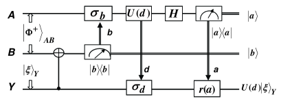
Figure 1: Quantum circuit of the simplified HPV protocol, where $U(d)$ is a quantum operation to be remotely implemented and it is diagonal or antidiagonal, $H$ is a Hadamard gate, $\sigma_{b},\sigma_{d}$ are identity matrices or not gates ($\sigma_{1}$) with respect to $b,d=0$ or $b,d=1$, respectively, and $r(a)=(1-a)\sigma_{0}+a\sigma_{3}$ is an identity matrix when $a=0$ or a phase gate ($\sigma_{3}$) when $a=1$. The measurements $\left|{a}\right\rangle$$\left\langle{a}\right|$ and $\left|{b}\right\rangle$$\left\langle{b}\right|$ are carried out in the computational basis ($a,b=0,1$). “$\Rightarrow$” (crewel with an arrow) indicates the transmission of classical communication to the location of the arrow direction.

In order to extend the RIO protocol to the cases of multiqubits, we first have to seek for the correct restricted sets of quantum operations of multiqubits that can be remotely implemented in a faithful and determined way. Actually, we have obtained their general and explicit forms in our recent works MyRIO , that is, the restricted sets of quantum operations of $N$ qubits have such forms that every row and every column of operations belonging to them only has one nonzero element. Thus, it is easy to know that there are $2^{N}!$ restricted sets of operations in the $N$-qubit systems. Denote the $x$th restricted set by $T^{r}_{N}(x,t)$, and its nonzero element in the $m$th row by $t_{m}$, we have

$$T^{r}_{N}(x,t)=\sum_{m=1}^{2^{N}}t_{m}\mbox{$\left|{m,D}\right\rangle$}\mbox{$\left\langle{p_{m}(x),D}\right|$}.$$ (5)

Here, $x=1,2,\cdots,2^{N}$ and

$$p(x)=(p_{1}(x),p_{2}(x),\cdots,p_{2^{N}}(x))$$ (6)

is an element belonging to the set of all permutations for the list $\{1,2,\cdots,2^{N}\}$. Moreover, when the requirement of the unitary condition is introduced, $t_{m}$ will be taken as ${\rm e}^{{\rm i}\phi_{m}}$, and $\phi_{m}$ is real.

To remotely implement quantum operations belonging to the above restricted sets, the sender(s) needs a mapping table which provides one-to-one mapping from $T^{r}_{N}(x,t)$ to a classical information $x$ $(x=1,2\cdots,2^{N}!)$, and the receiver knows a mapping table which gives out one-to-one mapping from a classical information $x$ $(x=1,2\cdots,2^{N}!)$ to $R_{N}(x)$ defined by

$${R}_{N}(x)=T_{N}^{r}(x,0)=\sum_{m=1}^{2^{N}}\mbox{$\left|{m,D}\right\rangle$}\mbox{$\left\langle{p_{m}(z),D}\right|$}.$$ (7)

Obviously, it has the same structure as $T_{N}^{r}(x,t)$ to be remotely implemented, and it is an important part in the final recovery operation.

For simplicity, let us consider the case of two qubits. It is clear that there are 24 kinds of restricted sets of quantum operations that can be remotely implemented. In our RIO protocol, we use two Bell states $|\Phi^{+}\rangle_{A_{1}B_{1}},|\Phi^{+}\rangle_{A_{2}B_{2}}$ as the quantum channel, where qubits $A_{1},A_{2}$ belong to Alice and $B_{1},B_{2}$ belong to Bob. Initially, an unknown state $|\xi\rangle_{Y_{1}Y_{2}}$ also belongs to Bob. Bob first performs two controlled-not ($C^{\rm not}$) transformation by using $Y_{1},Y_{2}$ as control qubits and $B_{1},B_{2}$ as target qubits, respectively. Then he measures his qubits $B_{1}$ and $B_{2}$ in the computational basis $|b_{1}\rangle_{B_{1}}\langle b_{1}|\otimes|b_{2}\rangle_{B_{2}}\langle b_{2}|$, where $b_{1},b_{2}=0,1$ and sends the results to Alice. After receiving the two classical bits, Alice first carries out the quantum operations $\sigma_{b_{1}}^{A_{1}}\otimes\sigma_{b_{2}}^{A_{2}}$ on her two qubits $A_{1},A_{2}$. Next Alice acts $T_{2}(x,t)$ on $A_{1}A_{2}$ and executes two Hadamard gate transformation $H_{A_{1}}\otimes H_{A_{2}}$. Then, she measures her two qubits in the basis $|a_{1}\rangle_{A_{1}}\langle a_{1}|\otimes|a_{2}\rangle_{A_{2}}\langle a_{2}|(a_{1},a_{2}=0,1)$ and sends the results $a_{1}a_{2}$ and $x$ to Bob. As we have mentioned, the transmission of $x$ is to let Bob choose $R_{2}(x)$ correctly. With these information, Bob’s recovery operations are taken as $\left[\mathfrak{r}^{Y_{1}}(a_{1})\otimes\mathfrak{r}^{Y_{2}}(a_{2})\right]{R}_{2}(x)$, where $\mathfrak{r}(y)=(1-y)\sigma_{0}+y\sigma_{3}$. Finally, our protocol is completed faithfully and determinedly through the above five steps.

III Controlled RIO in the cases of one qubit using one GHZ state

Now, let us first investigate the controlled remote implementations of quantum operations belonging to restricted sets of one qubit using one GHZ states. Without loss of generality, we can write the initial state in a symmetric form of three partite subsystems:

$$\mbox{$\left|{\Psi^{\rm ini}}\right\rangle$}=\mbox{$\left|{{\rm GHZ}_{+}}\right\rangle$}_{ABC}\mbox{$\left|{\chi}\right\rangle$}_{X}\mbox{$\left|{\xi}\right\rangle$}_{Y}\mbox{$\left|{\zeta}\right\rangle$}_{Z},$$ (8)

where the GHZ state has the form

$$\mbox{$\left|{{\rm GHZ}_{+}}\right\rangle$}=\frac{1}{\sqrt{2}}\left(\mbox{$\left|{000}\right\rangle$}+\mbox{$\left|{111}\right\rangle$}\right).$$ (9)

It is shared by Alice, Bob and Charlie. While $\mbox{$\left|{\chi}\right\rangle$}_{X}$, $\mbox{$\left|{\xi}\right\rangle$}_{Y}$ and $\mbox{$\left|{\zeta}\right\rangle$}_{Z}$ are all unknown states of one qubit system. The six qubits of the joint system are divided into three pairs, in which, the qubits $A$ and $X$ belong to Alice, the qubits $B$ and $Y$ belong to Bob, and the qubits $C$ and $Z$ belong to Charlie. Obviously, their roles are initially symmetric for the remote implementations of quantum operations of one qubit.

In order to clearly express our protocol and strictly prove it, specially, for the cases of multiqubits, we denote that the Hilbert space of the joint system is initially taken as a direct product of all qubit Hilbert spaces according to the following sequence:

$$H=H_{A}\otimes H_{B}\otimes H_{C}\otimes H_{X}\otimes H_{Y}\otimes H_{Z}.$$ (10)

We can simply call this direct-product “space structure” and denote it by a bit-string, for example, the space structure of the above Hilbert space is $ABCXYZ$. Note that the above space structure is only a notation rule used here, it is absolutely not a precondition of the protocols. If we would like to prove our protocols generally for the cases of multiqubits, such a kind of notation rule is convenient. This fact can be seen in Appendix A. Obviously, since taking such a space structure, the subspaces belonging to Alice, or Bob, or Charlie are separated. This will lead to inconvenience in the whole-space expression of local operations. Therefore, there is the need to change the space structure. This can be realized by a series of swapping transformations, which is studied in Appendix A.

In our protocols, in spite that only local operations and classical communication are used, the problems we deal with are related with the whole system because there is entanglement among various partite subsystems. However, knowing the space structure will be helpful for us to understand the effect of local operations. In fact, our protocol can be found due partially to the reasons that we clearly express an appreciate space structure and general swapping transformations. Therefore, in the following we keep the above sequence of direct products of qubit spaces via the whole-space expressions of our formula in the joint system.

From the symmetric initial state (8), it is easy to find that any one partite subsystem of them plays a possible role among of a sender, a receiver and a controller in the protocols. In other words, when a controller is fixed to a given partite subsystem, thus, the other two partite subsystems play a sender and a receiver, respectively. Under a controller’s permission, the remote implementations of quantum operations belonging to the restricted sets is faithfully and determinedly completed between the other two subsystems (locations).

Actually, we are always able to swap their positions in a given space structure among three partite subsystems using so-called general swapping transformations that are studied in Appendix A. Without loss of generality, as soon as a controller is chosen or dominated, we can rewrite the initial state space structure as

$$H_{\rm Controller}\otimes H_{\rm Sender}\otimes H_{\rm Receiver}\otimes H_{\rm Unknown\;\;State}.$$ (11)

This means that the first qubit belongs to the controller, the second qubit is in the sender’s partite subsystem (the local subsystem), the third qubit is mastered by the receiver, and the fourth qubit is an unknown state in the receiver’s hands. Obviously, the unknown states belong to sender and controller are needless in the protocol as soon as the roles of attendees are fixed.

When introducing a controller, our protocol of controlled remote implementations of quantum operations belonging to the restricted sets is made up of seven steps, in which, there are four steps of quantum operations including measurement and three times of classical communications. They are described as the following:

Controlling Step: This step is carried out by the controller. He/She performs a Hadamard transformation

$$H=\frac{1}{\sqrt{2}}\left(\begin{array}[]{cc}1&1\\ 1&-1\end{array}\right)$$ (12)

on his/her controlled qubit $\left|{\gamma}\right\rangle$, and then measures it in the computational basis $\mbox{$\left|{\gamma}\right\rangle$}\mbox{$\left\langle{\gamma}\right|$}\;(\gamma=0,1)$, that is

$$\mathcal{C}(\gamma) = \left(\mbox{$\left|{\gamma}\right\rangle$}\mbox{$\left\langle{\gamma}\right|$}H\right)\otimes I_{8},$$ (13)

where $I_{m}$ is a $m$ dimensional identity matrix.

This step is a key matter in our protocol. In fact, when the controller has not done it, there is no quantum entanglement between any two partite subsystems, so there is no any feasible remote implementations of operations. Only if a controller agrees or wishes that the other two partite subsystems implement the RIO protocol, he/she carries out this operation and measurement. Its action is to open the quantum channel between the sender and receiver that is necessary for the remote implementation of operations belonging to the restricted sets in a faithful and determined way.

Allowing Step: This step is still completed by the controller, that is, he/she transfers one ${c}$-bit $\bm{\gamma}$ to the sender or the receiver, which is denoted by $C_{\rm cs}(\gamma)$ or $C_{\rm cr}(\gamma)$, respectively.

This allowing step as well as the above controlling step can be arranged at any time in the RIO process, however, the different arrangement will result in influences on the steps of our protocols. If the classical bit $\gamma$ is arranged to transfer to the sender, this communication has to be done before the other parts of sending operations. If the classical bit $\gamma$ is chosen to transfer to the receiver, this communication is able to be done at the beginning (before receiver’s preparation), or in the middle (before the recovered operations), or at the end (after the standard recovered operations). At these cases, although the receiver can have the different choices to finish the protocol, we prefer to use a unified method for the RIO of one qubit, that is, we use the classical information $\gamma$ before the end of our protocol.

This step can be understood figuratively as that the controller distributes the “password” $\gamma$ to one of the sender and receiver, or gives an authorization to one of them, or says last word (to the receiver) in our protocols. This indicates the role of controller is very important and indispensable. Without the password distribution by the controller, the sender and receiver cannot faithfully and determinedly complete the RIO. This can be clearly seen in the following proofs about our protocols.

Preparing Step: This step is carried out by the receiver. There are two kinds of cases, respectively, based on whether the classical information from the controller is obtained by the receiver or not.

$\diamond$ Case one: If the receiver does not obtain the classical information from the controller, he/she first performs a controlled-not using his/her the qubit occupied by the unknown state as a control, his/her shared part (the qubit $\left|{\beta}\right\rangle$) of the GHZ state as a target, and then measures his/her shared part of the GHZ state in the computational basis $\mbox{$\left|{\beta}\right\rangle$}\mbox{$\left\langle{\beta}\right|$}\;(\beta=0,1)$, that is

$$\mathcal{P}(\beta) = I_{4}\otimes\left[\left(\mbox{$\left|{\beta}\right\rangle$}\mbox{$\left\langle{\beta}\right|$}\right)\otimes\sigma_{0}\right]\left[\sigma_{0}\otimes\left(\mbox{$\left|{0}\right\rangle$}\mbox{$\left\langle{0}\right|$}\right)+\sigma_{1}\otimes\left(\mbox{$\left|{1}\right\rangle$}\mbox{$\left\langle{1}\right|$}\right)\right]$$ (14)

$$= I_{4}\otimes\left[\left(\mbox{$\left|{\beta}\right\rangle$}\mbox{$\left\langle{\beta}\right|$}\right)\otimes\sigma_{0}\right]C^{\rm not}(2,1),$$

where $\sigma_{0}$ is $2\times 2$ identity matrix and $\sigma_{i}$ $(i=1,2,3)$ are the Pauli matrices, and $C^{\rm not}$ is a controlled-not defined by

$$C^{\rm not}(2,1)=\sigma_{0}\otimes\left(\mbox{$\left|{0}\right\rangle$}\mbox{$\left\langle{0}\right|$}\right)+\sigma_{1}\otimes\left(\mbox{$\left|{1}\right\rangle$}\mbox{$\left\langle{1}\right|$}\right)=\left(\begin{array}[]{cccc}1&0&0&0\\ 0&0&0&1\\ 0&0&1&0\\ 0&1&0&0\end{array}\right).$$ (15)

while $(2,1)$, as the variable of $C^{\rm not}$, indicates that the second qubit is a control and the first qubit is a target.

The purpose of this step is to let the unknown state be correlated with the sender’s local qubit. This is a precondition that the sender is able to remotely implement a quantum operation belonging to the restricted sets.

$\diamond$ Case two: If the controlling step has happened and the receiver gets the classical bit $\gamma$ from the controller, the preparing step has three different forms according to the time to obtain the classical bit $c$ in general.

(1) When the classical bit $\gamma$ is known at the beginning of this step, the receiver has to add a prior operation

$$\mathcal{P}^{\rm pre}(\gamma)=I_{4}\otimes\left[(1-\gamma)\sigma_{0}+\gamma\sigma_{3}\right]\otimes\sigma_{0}=I_{4}\otimes\mathfrak{r}(\gamma)\otimes\sigma_{0}$$ (16)

before the above operation (14). Here $\mathfrak{r}(a)$ is a diagonal phase gate with a parameter that is defined by

$$\mathfrak{r}(z)=(1-z)\sigma_{0}+z\sigma_{3}=\left(\begin{array}[]{cc}1&0\\ 0&1-2z\end{array}\right)=\left(\begin{array}[]{cc}1&0\\ 0&(-1)^{z}\end{array}\right).$$ (17)

Note that $z=0,1$, and then $(-1)^{z}=1-2z$. Of course, since it commutes with the project measurement, it also can be inserted between the measurement and the controlled not in the operation (14).

(2) When the classical bit $\gamma$ is known after the operation (14) or before next recovery operation, the receiver performs a supplementary operation

$$\mathcal{P}^{\rm aft}(\gamma)=I_{4}\otimes\mathfrak{r}(\gamma)\otimes\mathfrak{r}(\gamma),$$ (18)

where we have used the fact that

$$\left(\mathfrak{r}(\gamma)\otimes\mathfrak{r}(\gamma)\right)\left[\left(\mbox{$\left|{\beta}\right\rangle$}\mbox{$\left\langle{\beta}\right|$}\otimes\sigma_{0}\right)C^{\rm not}(2,1)\right]=\left[\left(\mbox{$\left|{\beta}\right\rangle$}\mbox{$\left\langle{\beta}\right|$}\otimes\sigma_{0}\right)C^{\rm not}(2,1)\right]\left(\mathfrak{r}(\gamma)\otimes\sigma_{0}\right).$$ (19)

(3) When the classical bit $\gamma$ is known after the next recovery operation, this case is discussed putting in the following recovery step. It is clear that for the above two cases, the receiver always can delay using the classical information up to after recovery operation. Therefore, this case is more general. However, it will be seen that the delaying method is able to lead in the unexpected complication in the recovery step for the cases of multiqubits.

Classical Communication from receiver to the sender: This step is that the receiver transfers a $c$-bit $\bm{\beta}$ to the sender, which is denoted by $C_{\rm rs}(\beta)$.

The aim of this step is that the receiver tells the sender that he/she is ready for receiving the remote operation, as well as his/her preparing way.

It must be emphasized that for the cases of one qubit, the receiver’s preparing has two equivalent ways with respect to $\beta=0$ or $1$, respectively. If the receiver first fixes the value of $\beta$ and tells the sender before the beginning of protocol, this step can be saved. In particular, when $\beta$ is just taken as $0$, the sender also does not need the transformation $\sigma_{\beta}$ in the next step, since $\sigma_{0}$ is trivial.

Sending step: This step is carried out by the sender. There are two cases.

$\diamond$ Case one: There is no classical information transferred from the controller to the sender. Thus, after receiving a classical bit $\beta$ from the receiver, the sender carries out her/his sending operations which are made of four parts (or five parts in the case two). The first one is simple $\sigma_{\beta}$

$$\mathcal{P}_{S}(\beta)=I_{2}\otimes\sigma_{\beta}\otimes I_{4}.$$ (20)

The second part of sending step is the operation $U(d,u)$ to be remotely implemented acting on his/her local system (the qubit $\left|{\alpha}\right\rangle$, a shared part of the GHZ state). The third part of sending step is simple a Hadamard gate. The fourth, also the final part is a measurement on the computational basis $\mbox{$\left|{\alpha}\right\rangle$}\mbox{$\left\langle{\alpha}\right|$}\;(\alpha=0,1)$. All parts of Alice’s sending can be jointly written as

$$\mathcal{S}(\alpha,\beta;d,u)=\left\{\sigma_{0}\otimes\left(\mbox{$\left|{\alpha}\right\rangle$}\mbox{$\left\langle{\alpha}\right|$}\right)\left[HU(d,u)\sigma_{\beta}\right]\otimes I_{4}\right\}.$$ (21)

The action of the first part $\sigma_{\beta}$ is to perfectly prepare the state of joint system as such a superposition that the basis in the locally acted system (belonging to sender’s subsystem) of every component state is the same as its basis in the remotely operated system (belonging to the space of unknown state in Bob’s subsystems) and the corresponding coefficients are just ones of unknown state.

The second part of sending step is just an operation belonging to the restricted sets, which will be remotely implemented in our protocol.

The third part of sending step, the Hadamard gate, is often seen in quantum computation and quantum communication. Its action is similar to the cases in the teleportation of states.

The fourth part of sending step is a measurement on the computational basis whose aim is to project to the needed result.

$\diamond$ Case two: The sender obtains the classical information $\gamma$ from the controller, he/she has to add to a prior operation

$$\mathcal{S}^{\rm add}(\gamma)=\sigma_{0}\otimes\left[(1-\gamma)\sigma_{0}+\gamma\sigma_{3}\right]\otimes I_{4}=\sigma_{0}\otimes\mathfrak{r}(\gamma)\otimes I_{4}$$ (22)

at the beginning of this step. This means that the sending step becomes

$$\mathcal{S}^{\rm all}(\alpha,\beta,\gamma;d,u)=\left\{\sigma_{0}\otimes\left(\mbox{$\left|{\alpha}\right\rangle$}\mbox{$\left\langle{\alpha}\right|$}\right)\left[HU(d,u)\sigma_{\beta}\right]\otimes I_{4}\right\}\mathcal{S}_{A}^{\rm add}(\gamma).$$ (23)

Classical Communication from sender to receiver: This step is that the sender transfers the classical information $\alpha$ and $d$ to the receiver, which is denoted by $C_{\rm sr}(\alpha;d)$.

This step is that sender tells the receiver what measurement (denoted by $\alpha$) has been done and which kind of operations (denoted by $d$) has been transferred. In our protocol, the sender has a one to one mapping table to indicate a kind of restrict set by a value of classical information. For the cases of one qubit, it can be encoded by one $c$-bit, in which, 0 denotes a restricted set of diagonal operations and 1 denotes a restricted set of antidiagonal operations.

Recovery Step: This step is carried out by the receiver. After receiving a classical bit $\alpha$ from the sender, the receiver first requires to do a recovery operation that consists of two parts or three parts. The first part is $\mathfrak{r}(\alpha)$ and the second part is a fixed form of a restricted set which has the same structure as the $U(d,u)$ to be transferred remotely but its nonzero elements are set as 1. For the cases of one qubit, the fixed forms of the restricted sets of diagonal- and antidiagonal operations are, respectively, $\sigma_{0}$ and $\sigma_{1}$. Therefore, the receiver’s recovery operations are written as

$${\mathcal{R}}(\alpha;d)=I_{8}\otimes\left[\mathfrak{r}(\alpha)\sigma_{d}\right],$$ (24)

where $d=0$ or $1$.

It must be emphasized that the above ${\mathcal{R}}(\alpha;d)$ only can guarantee the operation $U(d,u)$ is faithfully and determinedly transferred, if the protocol sets that the controller transfers his/her classical bit $\gamma$ before its action. Just as statement above, if $\gamma$ is transferred to the sender, the sender has a prior preparation part; when $\gamma$ is sent to the receiver before the his/her preparing step, he/she can add a supplementary part at the beginning, in the middle or at the end of the preparing step. Obviously, at the end of the preparing is just before the recovering, and so we can move this supplementary part to here. However, if the receiver obtains $\gamma$ from the controller after the above ${\mathcal{R}}(\alpha;d)$ action, the receiver has to perform an additional recovery part

$${\mathcal{R}}^{\rm aft}(\gamma;d)=(-1)^{\gamma d}I_{4}\otimes\mathfrak{r}(\gamma)\otimes\mathfrak{r}(\gamma),$$ (25)

where $\mathfrak{r}(z)$ is defined in Eq. (17). Note that $\mathfrak{r}(\gamma)\mbox{$\left|{\beta}\right\rangle$}\mbox{$\left\langle{\beta}\right|$}=(-1)^{\gamma\beta}\mbox{$\left|{\beta}\right\rangle$}\mbox{$\left\langle{\beta}\right|$}$, we obtain its another form

$${\mathcal{R}}^{\rm aft}(\beta,\gamma;d)=(-1)^{\gamma(d+\beta)}I_{8}\otimes\mathfrak{r}(\gamma).$$ (26)

It is clear that when the protocol sets the controller transfers his/her classical bit $\gamma$ to the receiver, we always can delay using the classical information $\gamma$. In other words, in order to standardize the protocol in the cases of one qubit, we do not add any $\mathcal{P}^{pre}$ and $\mathcal{P}^{aft}$ in the preparing step, but we always use the above ${\mathcal{R}}^{\rm aft}$ at the end of the protocol. Thus, the whole recovery operations are

$$\mathcal{R}^{\rm all}(\alpha,\gamma,d)={\mathcal{R}}^{\rm aft}(\gamma;d){\mathcal{R}}(\alpha;d).$$ (27)

However, for the case of multiqubits, it is not so simple. Generally, we put the additional recovery operations before the standard recovery operations (24), even before the preparing step in order to have the simplest additional operations for the cases of multiqubits. Of course, if we persist put the additional recovery operation in the last, we will pay a price that it gets a little complication in expressing.

In summary, when there is a controller, we have propose four kinds of protocols for controlled remote implementation of operations belonging to the restricted sets. (1) the sender obtains password; (2)-(4) the receiver obtains password respectively before the preparing, after the preparing (before the recovering) and after the recovering. The second, third and fourth kinds of our protocols can be unitedly expressed without obvious difficulty in the case of one qubit. If the controller transfers his classical bit $\gamma$ to the sender, the sequence of the above steps in our protocol will become

$$\mathcal{C}(\gamma)\rightarrow C_{\rm cs}(\gamma)\rightarrow\mathcal{P}(\beta)\rightarrow C_{\rm rs}(\beta)\rightarrow\mathcal{S}^{\rm all}(\alpha,\beta,\gamma;d)\rightarrow C_{\rm sr}(\alpha;d)\rightarrow\mathcal{R}(\alpha;d),$$ (28)

if the controller transfers his classical bit $\gamma$ to the receiver, the sequence of the above steps in our protocol is

$$\mathcal{C}(\gamma)\rightarrow C_{\rm cr}(\gamma)\rightarrow\mathcal{P}(\beta)\rightarrow C_{\rm rs}(\beta)\rightarrow\mathcal{S}(\alpha,\beta;d)\rightarrow C_{\rm sr}(\alpha;d)\rightarrow\mathcal{R}^{\rm all}(\alpha,\gamma;d).$$ (29)

It is clear that transferring $\gamma$ to the sender or the receiver can be figuratively understood as distributing a “password”, in special, while transferring $\gamma$ to the receiver at the end of protocol, it can be figuratively understood as “saying last word”. They are both important controlled means. Besides the password distributing, the controller owns the right to open the quantum channel. All of this are some main features of a controlled process. Therefore, we called the above process as a controlled remote implementations of operations.

Now, as an example, we fix the controller as Charlie, Alice as a sender and Bob as a receiver without loss of generality. Thus, the initial state is simplified as

$$\mbox{$\left|{\Psi_{ABCY}^{\rm ini}}\right\rangle$}=F^{-1}_{4}(1,3)\left[\mbox{$\left|{{\rm GHZ}_{+}}\right\rangle$}_{CAB}\mbox{$\left|{\xi}\right\rangle$}_{Y}\right],$$ (30)

where $F_{3}(1,3)$ is a forward rearrangement made of two swapping transformations between the neighbor qubits, which is defined in Appendix A. Similarly, we can discuss the other choices of the controller, sender and receiver, but we do not intend to discuss here.

If we set that the Charlie (controller) transfers the password to sender. It is the first kind of our protocols. All of the operations and measurements in our protocol can be jointedly written as

$$\mathcal{I}_{R}(a,b,c;d) = F^{-1}_{4}(1,3)\left\{\left(\mbox{$\left|{c}\right\rangle$}_{C}\mbox{$\left\langle{c}\right|$}H^{C}\right)\otimes\left(\mbox{$\left|{a}\right\rangle$}_{A}\mbox{$\left\langle{a}\right|$}H^{A}U(d,u)\sigma_{b}^{A}\mathfrak{r}(c)\right)\right.$$ (31)

$$\left.\otimes\left[\left(\sigma_{0}\otimes\mathfrak{r}(a)\right)C^{\rm not}\right]\right\}F_{4}(1,3).$$

Note that the operations with the superscripts $A,C$ denote their Hilbert spaces belonging, respectively, to the spaces of qubits $A,C$. Sometimes, if there is no any confusion, we omit these superscripts. This whole space form of our protocol has covered up the sequence of operations and steps of classical communication, but its advantage is clear. Its action on the initial state (30) yields

$$\mbox{$\left|{\Psi_{ABCY}^{\rm final}(a,b,c;d)}\right\rangle$}={\mathcal{I}}_{R}(a,b,c;d)\mbox{$\left|{\Psi_{ABCY}^{\rm ini}}\right\rangle$}=\frac{1}{2\sqrt{2}}\mbox{$\left|{abc}\right\rangle$}_{ABC}\otimes U(d,u)\mbox{$\left|{\xi}\right\rangle$}_{Y}.$$ (32)

The unknown state to be remotely implemented is just $\mbox{$\left|{\xi}\right\rangle$}_{Y}$ in Bob’s partite subsystem defined by Eq.(3). Our protocol is then determinedly and faithfully completed.

When setting that Charlie’s information transfers to Alice, the whole process of controlled remote implementation of quantum operations belonging to the restricted sets is shown in Fig.2.

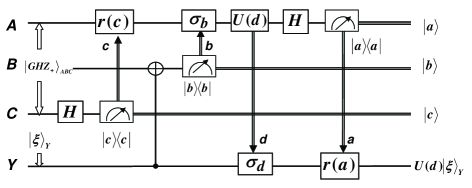
Figure 2: Quantum circuit of the controlled remote implementations of quantum operations with a controller Charlie. Here, $U(d)$ belonging to the restricted sets is a quantum operation to be remotely implemented, $H$ is a Hadamard transformation, $\sigma_{b},\sigma_{d}$ are identity matrices or not gates ($\sigma_{1}$) for $b,d=0$ or $b,d=1$ respectively, and $r(x)=(1-x)\sigma_{0}+x\sigma_{3}$ is equal an identity matrix if $x=0$ or a phase gate if $x=1$. The measurements $\left|{a}\right\rangle$$\left\langle{a}\right|$,$\left|{b}\right\rangle$$\left\langle{b}\right|$ and $\left|{c}\right\rangle$$\left\langle{c}\right|$ are carried out in the computational basis ($a,b,c=0,1$). “$\Rightarrow$” (crewel with an arrow) indicates the transmission of classical communication to the location of arrow direction.

Here, we only express the full operations for the first kind of our protocols, and provide its figure of quantum circuit. For the other three kinds of our protocols, the full operations and the figures of quantum circuits are similar. In addition, we should notice that the controller cannot choose who is a sender and who is a receiver in the other two partite subsystems. In other words, when Charlie is a controller, either of Alice and Bob can be chosen as a sender and the other one partite subsystem plays a receiver.

In the end of this section, let us prove our above protocol in detail. For simplicity, we only consider the cases that Alice is a sender, Bob is taken as a receiver, and Charlie is a controller. Initially, the joint system is in the state (30). When Charlie agrees or wishes that Alice and Bob can carry out the remote implementations of quantum operations belonging the restricted sets, he will open the quantum channel between them by preforming the controlling operation on his qubit. His action gives

$$\left|{\Psi_{ABCY}^{C}(c)}\right\rangle = F^{-1}_{4}(1,3)\mathcal{C}(c)F_{4}(1,3)\mbox{$\left|{\Psi^{\rm ini}_{ABCY}}\right\rangle$}$$ (33)

$$= \frac{1}{2}F^{-1}_{4}(1,3)\left[\mbox{$\left|{c}\right\rangle$}_{C}\otimes\left(\mbox{$\left|{00}\right\rangle$}_{AB}+(-1)^{c}\mbox{$\left|{11}\right\rangle$}_{AB}\right)\otimes\mbox{$\left|{\xi}\right\rangle$}_{Y}\right]$$

$$= \frac{1}{2}F^{-1}_{4}(1,3)\left(\sigma_{0}\otimes\mathfrak{r}(c)\otimes I_{4}\right)\left[\mbox{$\left|{c}\right\rangle$}_{C}\otimes\left(\mbox{$\left|{00}\right\rangle$}_{AB}+\mbox{$\left|{11}\right\rangle$}_{AB}\right)\otimes\mbox{$\left|{\xi}\right\rangle$}_{Y}\right]$$ (34)

$$= \frac{1}{2}F^{-1}_{4}(1,3)\left(I_{4}\otimes\mathfrak{r}(c)\otimes\sigma_{0}\right)\left[\mbox{$\left|{c}\right\rangle$}_{C}\otimes\left(\mbox{$\left|{00}\right\rangle$}_{AB}+\mbox{$\left|{11}\right\rangle$}_{AB}\right)\otimes\mbox{$\left|{\xi}\right\rangle$}_{Y}\right],$$ (35)

where we have used the definition of $\mathfrak{r}(y)$ in Eq. (17). Thus, Alice and Bob now share a Bell state, and they can carry out the protocol of RIO. However, because HPV protocol is dependent on the type of Bell state, Charlie has to send the “password” $c$ to Alice or Bob. Actually, this indicates the Charlie has his control right.

We need to consider two cases.

The first case is that the protocol sets Charlie to transfer his classical information $c$ to Alice. Using $\mathcal{P}(b)$, Bob prepares his state as

$$\left|{\Psi_{ABCY}^{P}(b,c)}\right\rangle = F^{-1}_{4}(1,3)\mathcal{P}(b)F_{4}(1,3)\mbox{$\left|{\Psi^{C}_{ABCY}}\right\rangle$}$$ (36)

$$= \frac{1}{2}\left[F^{-1}_{4}(1,3)\left(I_{2}\otimes\mathfrak{r}(c)\otimes I_{4}\right)\right]\mbox{$\left|{c}\right\rangle$}_{C}\otimes\left\{\sigma_{0}\otimes\left[\left(\mbox{$\left|{b}\right\rangle$}\mbox{$\left\langle{b}\right|$}\otimes\sigma_{0}\right)C^{\rm not}\right]\right\}$$

$$\times\left[\sum_{k=0}^{1}y_{k}\left(\mbox{$\left|{00k}\right\rangle$}_{ABY}+\mbox{$\left|{11k}\right\rangle$}_{ABY}\right)\right].$$

Note that

$$\left\{\sigma_{0}\otimes\left[\left(\mbox{$\left|{b}\right\rangle$}\mbox{$\left\langle{b}\right|$}\right)C^{\rm not}(2,1)\right]\right\}\left[\left(\mbox{$\left|{00k}\right\rangle$}+\mbox{$\left|{11k}\right\rangle$}\right)\right]$$ (37)

$$= \left[\sigma_{0}\otimes\left(\mbox{$\left|{b}\right\rangle$}\mbox{$\left\langle{b}\right|$}\right)\otimes\sigma_{0}\right]\left\{\left(\mbox{$\left|{000}\right\rangle$}+\mbox{$\left|{110}\right\rangle$}\right)\delta_{k0}+\left(\mbox{$\left|{011}\right\rangle$}+\mbox{$\left|{101}\right\rangle$}\right)\delta_{k1}\right\}$$

$$= \left(\mbox{$\left|{0b0}\right\rangle$}\delta_{b0}+\mbox{$\left|{1b0}\right\rangle$}\delta_{b1}\right)\delta_{k0}+\left(\mbox{$\left|{0b1}\right\rangle$}\delta_{b1}+\mbox{$\left|{1b1}\right\rangle$}\delta_{b0}\right)\delta_{k1}$$

$$= \left[\mbox{$\left|{bb0}\right\rangle$}\left(\delta_{b0}+\delta_{b1}\right)\delta_{k0}+\mbox{$\left|{(1-b)b1}\right\rangle$}\left(\delta_{b1}+\delta_{b0}\right)\delta_{k1}\right]$$

$$= \left(\sigma_{b}\otimes I_{4}\right)\left(\delta_{k0}\mbox{$\left|{0b0}\right\rangle$}+\delta_{k1}\mbox{$\left|{1b1}\right\rangle$}\right)$$

$$= \left(\sigma_{b}\otimes I_{4}\right)\left(\delta_{k0}+\delta_{k1}\right)\mbox{$\left|{kbk}\right\rangle$}$$

$$= \left(\sigma_{b}\otimes I_{4}\right)\mbox{$\left|{kbk}\right\rangle$},$$

where we have used the facts that $\sigma_{b}\mbox{$\left|{b}\right\rangle$}=\mbox{$\left|{0}\right\rangle$}$ and $\sigma_{b}\mbox{$\left|{1-b}\right\rangle$}=\mbox{$\left|{1}\right\rangle$}$ for $b=0,1$. It results in

$$\left|{\Psi_{ABCY}^{P}(b,c)}\right\rangle = \frac{1}{2}\left[F^{-1}_{4}(2,4)\left(\mathfrak{r}(c)\sigma_{b}\otimes I_{8}\right)\right]\left[\left(y_{0}\mbox{$\left|{00}\right\rangle$}_{AY}+y_{1}\mbox{$\left|{11}\right\rangle$}_{AY}\right)\otimes\mbox{$\left|{bc}\right\rangle$}_{BC}\right].$$ (38)

After Bob is ready, he transfers a classical bit $b$ in order to tell Alice his preparing way. So Alice starts with a supplementary operation so that the state of joint system is perfectly ready via the (22), that is

$$\left|{\Psi^{P}_{f}(b,c)}\right\rangle = F^{-1}_{4}(1,3)\mathcal{S}_{A}^{\rm add}(c)F_{4}(1,3)\mbox{$\left|{\Psi^{P}_{ABCY}}\right\rangle$}$$ (39)

$$= \frac{1}{2}F^{-1}_{4}(2,4)\left[\left(\sigma_{b}\otimes\sigma_{0}\right)\left(y_{0}\mbox{$\left|{00}\right\rangle$}_{AY}+y_{1}\mbox{$\left|{11}\right\rangle$}_{AY}\right)\otimes\mbox{$\left|{b}\right\rangle$}_{B}\mbox{$\left|{c}\right\rangle$}_{C}\right].$$

Therefore, Alice’s sending step yields

$$\left|{\Psi^{S}(a,b,c;d)}\right\rangle = F^{-1}_{4}(1,3)\mathcal{S}^{\rm all}(a,b,c,d)F_{4}(1,3)\mbox{$\left|{\Psi^{P}_{ABCY}}\right\rangle$}$$ (40)

$$= \frac{1}{2}F^{-1}_{4}(2,4)\left\{\left[\sum_{k}^{1}y_{k}\mbox{$\left\langle{a}\right|$}HU(d,u)\mbox{$\left|{k}\right\rangle$}\mbox{$\left|{a}\right\rangle$}_{A}\mbox{$\left|{k}\right\rangle$}_{Y}\right]\otimes\mbox{$\left|{bc}\right\rangle$}_{BC}\right\}.$$

The second case is that the protocol sets Charlie to transfer his classical information $c$ to Bob. If Bob choose to first perform $\mathcal{P}^{\rm pre}$, then its action is the same as Alice’s. Therefore, when Alice finishes the sending operation, we also obtain Eq. (40). Note that $\mathcal{P}^{\rm aft}(c)\mathcal{P}(b)=\mathcal{P}(b)\mathcal{P}^{\rm pre}(c)$, we can, after $\mathcal{P}(b)$ acting, use $\mathcal{P}^{\rm aft}(c)$. From $\mathcal{R}(a;d)\mathcal{P}^{\rm aft}(c)=(-1)^{cd}\mathcal{P}^{\rm aft}(c)\mathcal{R}(a;d)$, this also means that Bob can delay the additional recovery operation to the end. It is clear that the results of three kinds of procedures are the same.

Now, Bob performs recovery operation (24). From the relation that $U(d,u)=U(0,u)\sigma_{d}$, and the facts that $U(0,u)=\sum_{j=0}^{1}u_{j}\mbox{$\left|{j}\right\rangle$}\mbox{$\left\langle{j}\right|$}$ and $\mathfrak{r}(a)=\sum_{l=0}^{1}(-1)^{al}\mbox{$\left|{l}\right\rangle$}\mbox{$\left\langle{l}\right|$}$, it follows that

$$\left|{\Psi^{\rm final}(a,b,c;d)}\right\rangle = F^{-1}_{4}(1,3)\mathcal{R}(a,d)F_{4}(1,3)\mbox{$\left|{\Psi^{S}_{ABCY}}\right\rangle$}$$ (41)

$$= \frac{1}{2}F^{-1}_{4}(2,4)\left\{\left[\sum_{k}^{1}y_{k}\mbox{$\left\langle{a}\right|$}HU(d,u)\mbox{$\left|{k}\right\rangle$}\mbox{$\left|{a}\right\rangle$}_{A}\left(\mathfrak{r}(a)\sigma_{d}\mbox{$\left|{k}\right\rangle$}_{Y}\right)\right]\otimes\mbox{$\left|{bc}\right\rangle$}_{BC}\right\}$$

$$= \frac{1}{2}\mbox{$\left|{a}\right\rangle$}_{A}\otimes F^{-1}_{3}(1,3)\left\{\left[\sum_{j=0}^{1}\sum_{k=0}^{1}\sum_{l=0}^{1}u_{j}y_{k}\mbox{$\left\langle{a}\right|$}H\mbox{$\left|{j}\right\rangle$}\right.\right.$$

$$\left.\left.\times\left(\mbox{$\left\langle{j}\right|$}\sigma_{d}\mbox{$\left|{k}\right\rangle$}(-1)^{al}\mbox{$\left\langle{l}\right|$}\sigma_{d}\mbox{$\left|{k}\right\rangle$}\right)\mbox{$\left|{l}\right\rangle$}_{Y}\right]\mbox{$\left|{bc}\right\rangle$}_{BC}\right\}.$$

Note that

$$\mbox{$\left\langle{j}\right|$}\sigma_{d}\mbox{$\left|{k}\right\rangle$}\mbox{$\left\langle{l}\right|$}\sigma_{d}\mbox{$\left|{k}\right\rangle$}=\mbox{$\left\langle{j}\right|$}\sigma_{d}\mbox{$\left|{k}\right\rangle$}\delta_{jl},$$ (42)

we have

$$\left|{\Psi^{\rm final}(a,b,c;d)}\right\rangle = \frac{1}{2}\mbox{$\left|{a}\right\rangle$}_{A}\otimes F^{-1}_{3}(1,3)\left\{\left[\sum_{j=0}^{1}\sum_{k=0}^{1}u_{j}y_{k}(-1)^{aj}\mbox{$\left\langle{a}\right|$}H\mbox{$\left|{j}\right\rangle$}\mbox{$\left\langle{j}\right|$}\sigma_{d}\mbox{$\left|{k}\right\rangle$}\mbox{$\left|{j}\right\rangle$}_{Y}\right]\otimes\mbox{$\left|{bc}\right\rangle$}_{BC}\right\}.$$ (43)

Since

$$(-1)^{aj}\mbox{$\left\langle{a}\right|$}H\mbox{$\left|{j}\right\rangle$}=\frac{1}{\sqrt{2}}$$ (44)

for any $a$ and $j$, the above equation becomes

$$\left|{\Psi^{\rm final}(a,b,c;d)}\right\rangle = \frac{1}{2\sqrt{2}}\mbox{$\left|{a}\right\rangle$}_{A}\otimes F^{-1}_{3}(1,3)\left\{\left[\sum_{j=0}^{1}\sum_{k=0}^{1}u_{j}y_{k}\mbox{$\left\langle{j}\right|$}\sigma_{d}\mbox{$\left|{k}\right\rangle$}\mbox{$\left|{j}\right\rangle$}_{Y}\right]\otimes\mbox{$\left|{bc}\right\rangle$}_{BC}\right\}$$ (45)

$$= \frac{1}{2\sqrt{2}}\mbox{$\left|{a}\right\rangle$}_{A}\otimes F^{-1}_{3}(1,3)\left\{\left[\sum_{k=0}^{1}y_{k}U(0,u)\sigma_{d}\mbox{$\left|{k}\right\rangle$}_{Y}\right]\otimes\mbox{$\left|{bc}\right\rangle$}_{BC}\right\}$$

$$= \frac{1}{2\sqrt{2}}\mbox{$\left|{abc}\right\rangle$}_{ABC}\otimes U(d,u)\mbox{$\left|{\xi}\right\rangle$}_{Y}.$$

That is, we obtain the conclusion (32) of our protocol. Therefore, we finish the proof our protocols of controlled RIO with a controller in the cases of one qubit.

IV Combined RIO in the case of one qubit using one GHZ state

Now, let us consider a quantum operation that is a product of two parts $\mathcal{U}_{2}$ and $\mathcal{U}_{1}$, that is, $\mathcal{U}=\mathcal{U}_{2}\mathcal{U}_{1}$. Assuming $\mathcal{U}_{1}$ and $\mathcal{U}_{2}$ both belong to the restricted sets, we can denote them by $U(d_{1},u)$ and $U(d_{2},v)$, respectively, in our notation. Thus, the remote implementation of $\mathcal{U}$ can be completed via sending $\mathcal{U}_{1}$ and $\mathcal{U}_{2}$ in turn by one sender in the known protocols Huelga2 ; MyRIO , but two shared Bell pairs are needed. However, we find that this task can be faithfully and determinedly completed by two senders via one GHZ state. Moreover, we will see that the RIO protocol with two senders using one GHZ state has higher security compared with one using two Bell states. More analysis about the security enhancement has been given in our introduction.

Without loss of generality, we set Alice and Bob as two senders, and Alice first sends $U(d_{1},u)$, Bob then sends $U(d_{2},v)$. Charlie plays a receiver. Except for the unknown state is replaced by $\mbox{$\left|{\zeta}\right\rangle$}=z_{0}\mbox{$\left|{0}\right\rangle$}_{Z}+z_{1}\mbox{$\left|{1}\right\rangle$}_{Z}$, the initial state has not the other difference form Eq. (30). Since the significance and actions of the most related operations have been explained in Sec. III, we do not intend to repeat them here. Our protocol is made of the following seven steps.

Step one: Charlie’s preparing.

$$\mathcal{P}_{C}(c)=I_{4}\otimes\left[\left(\mbox{$\left|{c}\right\rangle$}_{C}\mbox{$\left\langle{c}\right|$}\right)\otimes\sigma_{0}^{Z}\right]\left[\sigma_{0}^{C}\otimes\left(\mbox{$\left|{0}\right\rangle$}_{Z}\mbox{$\left\langle{0}\right|$}\right)+\sigma_{1}^{C}\otimes\left(\mbox{$\left|{1}\right\rangle$}_{Z}\mbox{$\left\langle{1}\right|$}\right)\right].$$ (46)

Step two: First classical communication. Charlie sends the classical information $c$ to Alice and Bob.

Step three: Alice’s sending.

$$\mathcal{S}_{A}(a,c;d_{1},u)=\left(\mbox{$\left|{a}\right\rangle$}_{A}\mbox{$\left\langle{a}\right|$}\right)\left[H^{A}U(d_{1},u)\right]\sigma_{c}^{A}\otimes I_{8}.$$ (47)

Step four: Second classical communication. Alice sends the classical information $d_{1}$ to Bob and $a$ to Charlie.

Step five: Bob’s sending.

$$\mathcal{S}_{B}(b,c;d_{1},d_{2},v)=\sigma_{0}\otimes\left(\mbox{$\left|{b}\right\rangle$}_{B}\mbox{$\left\langle{b}\right|$}\right)\left[H^{B}U(d_{2},v)\right]\left(\sigma_{d_{1}}^{B}\sigma_{c}^{B}\right)\otimes I_{4}.$$ (48)

Step six: Third classical communication. Bob sends the classical information $b$ and $d_{2}$ to Charlie.

Step seven: Charlie’s recovering

$${\mathcal{R}}_{C}(a,b;d_{1},d_{2})=I_{4}\otimes\sigma_{0}^{C}\otimes\left(\mathfrak{r}(b)\sigma_{d_{2}}\right).\left(\mathfrak{r}(a)\sigma_{d_{1}}\right).$$ (49)

All of the operations and measurements in our above protocol can be jointly written as

$$\mathcal{I}_{R}(a,b,c;d_{1},d_{2},u,v) = \left(\mbox{$\left|{a}\right\rangle$}_{A}\mbox{$\left\langle{a}\right|$}H^{A}U(d_{1},u)\sigma_{c}^{A}\right)\otimes\left(\mbox{$\left|{b}\right\rangle$}_{B}\mbox{$\left\langle{b}\right|$}H^{B}U(d_{2},v)\sigma_{d_{1}}\sigma_{c}^{A}\right)$$ (50)

$$\times\left[\left(\mbox{$\left|{c}\right\rangle$}\mbox{$\left\langle{c}\right|$}\otimes\mathfrak{r}(b)\sigma_{d_{2}}\mathfrak{r}(a)\sigma_{d_{1}}\right)C^{\rm not}\right].$$

Its acting on the initial state gives

$$\mbox{$\left|{\Psi_{C}^{\rm final}(a,b,c;d_{1},d_{2},u,v)}\right\rangle$}={\mathcal{I}}_{R}(a,b,c;d_{1},d_{2},u,v)\mbox{$\left|{\Psi_{C}^{\rm ini}}\right\rangle$}=\frac{1}{2\sqrt{2}}\mbox{$\left|{abc}\right\rangle$}_{ABC}\otimes U(d_{2},v)U(d_{1},u)\mbox{$\left|{\zeta}\right\rangle$}_{Z},$$ (51)

where $a,b,c=0,1$ denote the spin up or down, and $d_{1},d_{2}=0$ and $d_{1},d_{2}=1$ respectively indicate the operations of diagonal and antidiagonal restricted sets. Therefore, the remote implementations of the combination of two quantum operations belonging to restricted sets are faithfully and determinedly completed. It can be called the combined remote implementation of quantum operations which can be displayed by Fig.3.

Figure 3: Quantum circuit of the combined remote implementation of quantum operation with two sender Alice and Bob . Here, $U_{1}(d_{1})$ and $U_{2}(d_{2})$ are respectively a part of the quantum operation $U(d_{1},d_{2})=U_{2}(d_{2})U_{1}(d_{1})$ that is remotely implemented by combining Alice and Bob’s actions, $H$ is a Hadamard transformation, $\sigma_{c},\sigma_{d_{1}},\sigma_{d_{2}}$ are identity matrices or not gates ($\sigma_{1}$) for $c,d_{1},d_{2}=0$ or $c,d_{1},d_{2}=1$ respectively, and $r(x)=(1-x)\sigma_{0}+x\sigma_{3}$ is an identity matrix if $x=0$ or a phase gate ($\sigma_{3}$) if $x=1$. The measurements $\left|{a}\right\rangle$$\left\langle{a}\right|$,$\left|{b}\right\rangle$$\left\langle{b}\right|$ and $\left|{c}\right\rangle$$\left\langle{c}\right|$ are carried out in the computational basis ($a,b,c=0,1$). “$\Rightarrow$” (crewel with an arrow) indicates the transmission of classical communication to the location of arrow direction.

In order to prove our protocol with two senders, we first need the equation

$$\left\{\sigma_{0}\otimes\left[\left(\mbox{$\left|{c}\right\rangle$}\mbox{$\left\langle{c}\right|$}\otimes\sigma_{0}\right)C^{\rm not}(2,1)\right]\right\}\mbox{$\left|{\rm GHZ_{+}}\right\rangle$}\otimes\mbox{$\left|{k}\right\rangle$}=F^{-1}_{4}(3,4)\left(\sigma_{c}\otimes\sigma_{c}\otimes I_{4}\right)\left(\mbox{$\left|{kkk}\right\rangle$}\otimes\mbox{$\left|{c}\right\rangle$}\right).$$ (52)

Its proof is similar to Eq. (37). Therefore, Charlie’s preparation gives

$$\left|{\Psi^{P}(c)}\right\rangle = \mathcal{P}_{C}(c)\mbox{$\left|{\Psi^{\rm ini}_{ABCZ}}\right\rangle$}$$ (53)

$$= \frac{1}{\sqrt{2}}F^{-1}_{4}(3,4)\left[\left(\sigma_{c}\otimes\sigma_{c}\otimes I_{4}\right)\left(z_{0}\mbox{$\left|{00}\right\rangle$}_{AB}\otimes\mbox{$\left|{0}\right\rangle$}_{Y}+z_{1}\mbox{$\left|{11}\right\rangle$}_{AB}\otimes\mbox{$\left|{1}\right\rangle$}_{Y}\right)\otimes\mbox{$\left|{c}\right\rangle$}_{C}\right],$$

where $F_{N}(i,j)$ is defined in Appendix A.

After receiving the classical information $c$ from Charlie (receiver), Alice supplements a $\sigma_{c}$ transformation, and then performs the first sending operations, we have

$$\left|{\Psi_{1}^{S}(a,c;d_{1},u)}\right\rangle = \mathcal{S}_{A}(a,c,d_{1},u)\mbox{$\left|{\Psi^{P}(c)}\right\rangle$}$$ (54)

$$= \frac{1}{\sqrt{2}}F^{-1}_{4}(3,4)\left[\sum_{k=0}^{1}z_{k}(\mbox{$\left|{a}\right\rangle$}_{A}\mbox{$\left\langle{a}\right|$}HU(d_{1},u)\mbox{$\left|{k}\right\rangle$})\left(\sigma_{c}\mbox{$\left|{k}\right\rangle$}_{B}\right)\mbox{$\left|{k}\right\rangle$}_{Y}\right]\otimes\mbox{$\left|{c}\right\rangle$}_{C}.$$

Alice again tells Bob $d_{1}$ and Charlie $a$. In succession, based on the classical information $c$ (coming from Charlie) and $d_{1}$ (coming from Alice), Bob first carries out $\sigma_{d_{1}}\sigma_{c}$, and then performs the second sending operations:

$$\left|{\Psi_{2}^{S}(a,b,c;d_{1},d_{2},u,v)}\right\rangle = \mathcal{S}_{B}(b,c,d_{2},v)\mbox{$\left|{\Psi^{S}_{1}(a,c,d_{1},u}\right\rangle$}$$ (55)

$$= \frac{1}{\sqrt{2}}F^{-1}_{4}(3,4)\left[\sum_{k=0}^{1}z_{k}\left(\mbox{$\left|{a}\right\rangle$}_{A}\mbox{$\left\langle{a}\right|$}HU(d_{1},u)\mbox{$\left|{k}\right\rangle$}_{A}\right)\right.$$

$$\otimes\left.\left(\mbox{$\left|{b}\right\rangle$}_{B}\mbox{$\left\langle{b}\right|$}HU(d_{2},v)\sigma_{d_{1}}\mbox{$\left|{k}\right\rangle$}_{B}\right)\mbox{$\left|{k}\right\rangle$}_{Y}\right]\otimes\mbox{$\left|{c}\right\rangle$}_{C}.$$

Finally, Bob’s recovery operation gives

$$\left|{\Psi^{\rm final}(a,b,c;d_{1},d_{2},u,v)}\right\rangle = \mathcal{R}_{B}(a,b,d_{1},d_{2})\mbox{$\left|{\Psi^{S}_{2}(a,b,c,d_{1},d_{2},u,v}\right\rangle$}$$ (56)

$$= \frac{1}{\sqrt{2}}F^{-1}_{4}(3,4)\left[\sum_{k=0}^{1}z_{k}\left(\mbox{$\left|{a}\right\rangle$}_{A}\mbox{$\left\langle{a}\right|$}HU(d_{1},u)\mbox{$\left|{k}\right\rangle$}\right)\right.$$

$$\left.\times\left(\mbox{$\left|{b}\right\rangle$}_{B}\mbox{$\left\langle{b}\right|$}HU(d_{2},v)\sigma_{d_{1}}\mbox{$\left|{k}\right\rangle$}\right)\right.$$

$$\otimes\left.\mathfrak{r}(b)\sigma_{d_{2}}\mathfrak{r}(a)\sigma_{d_{1}}\mbox{$\left|{k}\right\rangle$}_{Z}\right]\otimes\mbox{$\left|{c}\right\rangle$}_{C}.$$

The remaining steps of this proof is similar to the ones in the end of Sec. III, but it needs to repeat three times. First, using $U(d_{1},u)=U(0,u)\sigma_{d_{1}}=\sum_{j=0}^{1}u_{j}\mbox{$\left|{j}\right\rangle$}\mbox{$\left\langle{j}\right|$}\sigma_{d_{1}}$ and $\mathfrak{r}(a)=\sum_{l=0}^{1}(-1)^{al}\mbox{$\left|{l}\right\rangle$}\mbox{$\left\langle{l}\right|$}$ we have

$$\left|{\Psi^{\rm final}(a,b,c;d_{1},d_{2},u,v)}\right\rangle = \frac{1}{\sqrt{2}}\left[\sum_{j=0}^{1}\sum_{k=0}^{1}\sum_{l=0}^{1}u_{j}y_{k}\left(\mbox{$\left|{a}\right\rangle$}_{A}\mbox{$\left\langle{a}\right|$}H\mbox{$\left|{j}\right\rangle$}\mbox{$\left\langle{j}\right|$}\sigma_{d_{1}}\mbox{$\left|{k}\right\rangle$}\right)\right.$$ (57)

$$\otimes\left(\mbox{$\left|{b}\right\rangle$}_{B}\mbox{$\left\langle{b}\right|$}HU(d_{2},v)\sigma_{d_{1}}\mbox{$\left|{k}\right\rangle$}\right)$$

$$\left.\otimes\mathfrak{r}(b)\sigma_{d_{2}}(-1)^{al}\mbox{$\left|{l}\right\rangle$}_{Y}\mbox{$\left\langle{l}\right|$}\sigma_{d_{1}}\mbox{$\left|{k}\right\rangle$}\right]\otimes\mbox{$\left|{c}\right\rangle$}_{C}.$$

Because that $\mbox{$\left\langle{j}\right|$}\sigma_{y}\mbox{$\left|{k}\right\rangle$}\mbox{$\left\langle{l}\right|$}\sigma_{d_{1}}\mbox{$\left|{k}\right\rangle$}=\delta_{jl}\mbox{$\left\langle{j}\right|$}\sigma_{y}\mbox{$\left|{k}\right\rangle$}$, it becomes

$$\left|{\Psi^{\rm final}(a,b,c;d_{1},d_{2},u,v)}\right\rangle = \frac{1}{\sqrt{2}}\mbox{$\left|{ab}\right\rangle$}_{AB}\otimes\left[\sum_{j=0}^{1}\sum_{k=0}^{1}u_{j}y_{k}\left(\mbox{$\left\langle{a}\right|$}H\mbox{$\left|{j}\right\rangle$}(-1)^{aj}\right)\right.$$ (58)

$$\times\left(\mbox{$\left\langle{b}\right|$}HU(d_{2},v)\sigma_{d_{1}}\mbox{$\left|{k}\right\rangle$}\right)\left.\mathfrak{r}(b)\sigma_{d_{2}}\mbox{$\left|{j}\right\rangle$}_{Y}\mbox{$\left\langle{j}\right|$}\sigma_{d_{1}}\mbox{$\left|{k}\right\rangle$}\right]\otimes\mbox{$\left|{c}\right\rangle$}_{C}.$$

While from $\mbox{$\left\langle{a}\right|$}H\mbox{$\left|{j}\right\rangle$}(-1)^{aj}=1/\sqrt{2}$, it follows that

$$\left|{\Psi^{\rm final}(a,b,c;d_{1},d_{2},u,v)}\right\rangle = \frac{1}{2}\mbox{$\left|{ab}\right\rangle$}_{AB}\otimes\left[\sum_{j=0}^{1}\sum_{k=0}^{1}u_{j}y_{k}\left(\mbox{$\left\langle{b}\right|$}HU(d_{2},v)\sigma_{d_{1}}\mbox{$\left|{k}\right\rangle$}\right)\right.$$ (59)

$$\times\left.\mathfrak{r}(b)\sigma_{d_{2}}\mbox{$\left|{j}\right\rangle$}_{Y}\mbox{$\left\langle{j}\right|$}\sigma_{d_{1}}\mbox{$\left|{k}\right\rangle$}\right]\otimes\mbox{$\left|{c}\right\rangle$}_{C}.$$

Again inserted the complete relation after $U(d_{2})$ and based on the above same reason, the above equation is reduced to

$$\left|{\Psi^{\rm final}(a,b,c;d_{1},d_{2},u,v)}\right\rangle = \frac{1}{2}\mbox{$\left|{ab}\right\rangle$}_{AB}\otimes\left[\sum_{j=0}^{1}\sum_{k=0}^{1}\sum_{l=0}^{1}u_{j}y_{k}\left(\mbox{$\left\langle{b}\right|$}HU(d_{2},v)\mbox{$\left|{l}\right\rangle$}\mbox{$\left\langle{l}\right|$}\sigma_{d_{1}}\mbox{$\left|{k}\right\rangle$}\right)\right.$$ (60)

$$\left.\times\mathfrak{r}(b)\sigma_{d_{2}}\mbox{$\left|{j}\right\rangle$}_{Y}\mbox{$\left\langle{j}\right|$}\sigma_{d_{1}}\mbox{$\left|{k}\right\rangle$}\right]\otimes\mbox{$\left|{c}\right\rangle$}_{C}$$

$$= \frac{1}{2}\mbox{$\left|{ab}\right\rangle$}_{AB}\otimes\left[\sum_{j=0}^{1}\sum_{k=0}^{1}u_{j}y_{k}\left(\mbox{$\left\langle{b}\right|$}HU(d_{2},v)\mbox{$\left|{j}\right\rangle$}\right)\right.$$

$$\left.\times\mathfrak{r}(b)\sigma_{d_{2}}\mbox{$\left|{j}\right\rangle$}_{Y}\mbox{$\left\langle{j}\right|$}\sigma_{d_{1}}\mbox{$\left|{k}\right\rangle$}\right]\otimes\mbox{$\left|{c}\right\rangle$}_{C}.$$

Repeatedly using the above skills, that is $U(d_{2})=U(0,v)\sigma_{d_{2}}=\sum_{i=0}^{1}v_{i}\mbox{$\left|{i}\right\rangle$}\mbox{$\left\langle{i}\right|$}\sigma_{d_{2}}$ and $\mathfrak{r}(b)=\sum_{l=0}^{1}(-1)^{bl}\mbox{$\left|{l}\right\rangle$}\mbox{$\left\langle{l}\right|$}$, we obtain

$$\left|{\Psi^{\rm final}(a,b,c;d_{1},d_{2},u,v)}\right\rangle = \frac{1}{2}\mbox{$\left|{ab}\right\rangle$}_{AB}\otimes\left[\sum_{i=0}^{1}\sum_{j=0}^{1}\sum_{k=0}^{1}\sum_{l=0}^{1}v_{i}u_{j}y_{k}\left(\mbox{$\left\langle{b}\right|$}H\mbox{$\left|{i}\right\rangle$}\mbox{$\left\langle{i}\right|$}\sigma_{d_{2}}\mbox{$\left|{j}\right\rangle$}\right)\right.$$ (61)

$$\left.\times(-1)^{bl}\mbox{$\left|{l}\right\rangle$}_{Y}\mbox{$\left\langle{l}\right|$}\sigma_{d_{2}}\mbox{$\left|{j}\right\rangle$}\mbox{$\left\langle{j}\right|$}\sigma_{d_{1}}\mbox{$\left|{k}\right\rangle$}\right]\otimes\mbox{$\left|{c}\right\rangle$}_{C}$$

$$= \frac{1}{2}\mbox{$\left|{ab}\right\rangle$}_{AB}\otimes\left[\sum_{i=0}^{1}\sum_{j=0}^{1}\sum_{k=0}^{1}v_{i}u_{j}y_{k}\left(\mbox{$\left\langle{b}\right|$}H\mbox{$\left|{i}\right\rangle$}(-1)^{bi}\right)\right.$$

$$\left.\times\mbox{$\left\langle{i}\right|$}\sigma_{d_{2}}\mbox{$\left|{j}\right\rangle$}\mbox{$\left\langle{j}\right|$}\sigma_{d_{1}}\mbox{$\left|{k}\right\rangle$}\mbox{$\left|{i}\right\rangle$}_{Y}\right]\otimes\mbox{$\left|{c}\right\rangle$}_{C}$$

$$= \frac{1}{2\sqrt{2}}\mbox{$\left|{ab}\right\rangle$}_{AB}\otimes\left[\sum_{i=0}^{1}\sum_{j=0}^{1}\sum_{k=0}^{1}v_{i}u_{j}y_{k}\mbox{$\left\langle{i}\right|$}\sigma_{d_{2}}\mbox{$\left|{j}\right\rangle$}\mbox{$\left\langle{j}\right|$}\sigma_{d_{1}}\mbox{$\left|{k}\right\rangle$}\mbox{$\left|{i}\right\rangle$}_{Y}\right]\otimes\mbox{$\left|{c}\right\rangle$}_{C}$$

$$= \frac{1}{2\sqrt{2}}\mbox{$\left|{ab}\right\rangle$}_{AB}\otimes\left[U(d_{2},v)U(d_{1},u)\mbox{$\left|{\xi}\right\rangle$}_{Y}\right]\otimes\mbox{$\left|{c}\right\rangle$}_{C}.$$

The proof of our protocol with two senders using one GHZ state is finished.

V Protocols in the cases of $N$ qubits

We have proposed and proved the protocols of controlled and combined remote implementations of quantum operations for one qubit using one GHZ state, respectively. The controlled RIO has a controller, a sender and a receiver, and the roles of three partite subsystems can be exchanged with each other. The combined RIO has two senders and a receiver, and every sender transfers an operation (or a part of one decomposable operation), two transferred operations are combined together according to the sequence of transferred time to form a total operation that is remotely implemented. In the following let us investigate the cases of multiqubits.

We have seen that since a controller or an extra sender being fetched in the protocols for the cases of one qubit, the entanglement resource really used to the remote implementations of operations is still one Bell pair, in spite that our protocols is carried out via one GHZ state. In other words, the design of adding controller or extra sender will use a part of the entanglement resource. Therefore, for the cases of more than one qubit, our restricted sets MyRIO are still suitable to our controlled and combined RIOs.

V.1 Some notations

Usually, in order to avoid the possible errors, we need to denote the sequential structure of direct product space of qubits, or a sequence of direct products of qubit space basis vectors in the multiqubit systems. For Alice’s space, we set its sequential structure as $A_{1}A_{2}\cdots A_{N}$, in other words, its basis vector has the form $\mbox{$\left|{a_{1}}\right\rangle$}_{A_{1}}\mbox{$\left|{a_{2}}\right\rangle$}_{A_{2}}\cdots\mbox{$\left|{a_{N}}\right\rangle$}_{A_{N}}$ (or $\mbox{$\left|{a_{1}a_{2}\cdots a_{N}}\right\rangle$}_{A_{1}A_{2}\cdots A_{N}}$). Similarly, we set the sequential structure of Bob’s space as $B_{1}B_{2}\cdots B_{N}Y_{1}Y_{2}\cdots Y_{N}$, in other words, its basis vector has the form $\mbox{$\left|{b_{1}}\right\rangle$}_{B_{1}}\mbox{$\left|{b_{2}}\right\rangle$}_{B_{2}}\cdots\mbox{$\left|{b_{N}}\right\rangle$}_{B_{N}}\mbox{$\left|{k_{1}}\right\rangle$}_{Y_{1}}\mbox{$\left|{k_{2}}\right\rangle$}_{Y_{2}}\cdots\mbox{$\left|{k_{N}}\right\rangle$}_{Y_{N}}$. It is clear that for a $N$-qubit system, its space structure can be represented by a bit-string with the length of $N$.

In order to write our formula compactly and clearly, and then prove our protocols more conveniently, we need to use some general swapping transformations, for example, $F_{N}(i,j)$, $P_{N}(j,k)$, $\Lambda(2,N)$, $\Omega(2,N)$, $\Omega(3,N)$ and $\Upsilon(3,N)$, that are studied in Appendix A and we will not repeatedly write their definitions here.

In addition, we still need to define

$$\Theta_{N}=\Omega(3,N)\Upsilon^{-1}(3,N)$$ (62)

and then introduce

$$\Theta_{A}(n)=\left(I_{2^{n}}\otimes\Lambda(2,N)\otimes I_{2^{N}}\right)\left(\Theta_{n}\otimes I_{2^{3N-2n)}}\right),$$ (63)

$$\Theta_{B}(n)=\left(I_{2^{n}}\otimes\Upsilon(3,N)\right)\left(\Theta_{n}\otimes I_{2^{3N-2n)}}\right),$$ (64)

$$\Theta_{C}(n)=\left(\Theta_{n}\otimes I_{2^{3N-2n)}}\right).$$ (65)

Thus, we have

$$\Theta_{A}(n)\left[\left(\bigotimes_{m=1}^{n}\mbox{$\left|{a_{m}b_{m}c_{m}}\right\rangle$}_{A_{m}B_{m}C_{m}}\right)\left(\bigotimes_{s=n+1}^{N}\mbox{$\left|{a_{s}b_{s}}\right\rangle$}_{A_{s}B_{s}}\right)\otimes\left(\bigotimes_{t=1}^{N}\mbox{$\left|{k_{t}}\right\rangle$}_{Y_{t}}\right)\right]$$

$$\quad=\left(\bigotimes_{m=1}^{n}\mbox{$\left|{c_{m}}\right\rangle$}_{C_{m}}\right)\left(\bigotimes_{s=n+1}^{N}\mbox{$\left|{a_{s}}\right\rangle$}_{A_{s}}\right)\left(\bigotimes_{m=1}^{N}\mbox{$\left|{b_{m}}\right\rangle$}_{B_{m}}\right)\otimes\left(\bigotimes_{m=1}^{N}\mbox{$\left|{k_{m}}\right\rangle$}_{Y_{m}}\right),$$ (66)

$$\Theta_{B}(n)\left[\left(\bigotimes_{m=1}^{n}\mbox{$\left|{a_{m}b_{m}c_{m}}\right\rangle$}_{A_{m}B_{m}C_{m}}\right)\left(\bigotimes_{s=n+1}^{N}\mbox{$\left|{a_{s}b_{s}}\right\rangle$}_{A_{s}B_{s}}\right)\otimes\left(\bigotimes_{s=1}^{N}\mbox{$\left|{k_{s}}\right\rangle$}_{Y_{s}}\right)\right]$$

$$\quad=\left(\bigotimes_{m=1}^{n}\mbox{$\left|{c_{m}}\right\rangle$}_{C_{m}}\right)\left(\bigotimes_{s=1}^{N}\mbox{$\left|{a_{s}b_{s}k_{s}}\right\rangle$}_{A_{s}B_{s}Y_{s}}\right),$$ (67)

$$\Theta_{C}(n)\left[\left(\bigotimes_{m=1}^{n}\mbox{$\left|{a_{m}b_{m}c_{m}}\right\rangle$}_{A_{m}B_{m}C_{m}}\right)\left(\bigotimes_{s=n+1}^{N}\mbox{$\left|{a_{s}b_{s}}\right\rangle$}_{A_{s}B_{s}}\right)\otimes\left(\bigotimes_{t=1}^{N}\mbox{$\left|{k_{t}}\right\rangle$}_{Y_{t}}\right)\right]$$

$$\quad=\left(\bigotimes_{m=1}^{n}\mbox{$\left|{c_{m}}\right\rangle$}_{C_{m}}\right)\left(\bigotimes_{s=1}^{N}\mbox{$\left|{a_{s}b_{s}}\right\rangle$}_{A_{s}B_{s}}\right)\otimes\left(\bigotimes_{t=1}^{N}\mbox{$\left|{k_{t}}\right\rangle$}_{Y_{t}}\right).$$ (68)

Similarly, we can obtain the transformed relations acting on the operations (or matrices).

By comparing with the cases of one qubit, we can extend the controlled and combined RIO protocols to the cases of $N$ qubits in terms of our restricted sets. However, we find that the variety of protocols is more obvious, the expressions and proofs of protocols get a little complicated. Our protocols are still made up of seven steps for controlled and combined remote implementations of $N$-qubit quantum operations belonging to our restricted sets. For the cases with $n<N$ controllers, we only need $n$ GHZ states and $N-n$ Bell pairs. While when two senders are fetched in, we need $N$ GHZ states.

Without loss of generality, when with $n$ controllers, we set the former $n$ shared entangled states as GHZ states, the initial state reads

$$\mbox{$\left|{\Psi_{N}^{\rm ini}}\right\rangle$}=\left(\bigotimes_{m=1}^{n}\mbox{$\left|{\rm GHZ^{+}}\right\rangle$}_{A_{m}B_{m}C_{m}}\right)\otimes\left(\bigotimes_{s=n+1}^{N}\mbox{$\left|{\Phi^{+}}\right\rangle$}_{A_{s}B_{s}}\right)\otimes\mbox{$\left|{\xi}\right\rangle$}_{Y_{1}Y_{2}\cdots Y_{N}},$$ (69)

when with two senders, we take the $N$ shared GHZ states, the initial state becomes

$$\mbox{$\left|{\Psi_{N}^{\rm ini}}\right\rangle$}=\left(\bigotimes_{m=1}^{N}\mbox{$\left|{\rm GHZ^{+}}\right\rangle$}_{A_{m}B_{m}C_{m}}\right)\otimes\mbox{$\left|{\xi}\right\rangle$}_{Y_{1}Y_{2}\cdots Y_{N}},$$ (70)

where $\mbox{$\left|{\xi}\right\rangle$}_{y_{1}Y_{2}\cdots y_{N}}$ is an arbitrary (unknown) pure state in the $N$-qubit systems:

$$\mbox{$\left|{\xi}\right\rangle$}_{Y_{1}\cdots Y_{N}}=\sum_{k_{1},\cdots,k_{N}=0}^{1}y_{k_{1}\cdots k_{N}}\mbox{$\left|{k_{1}k_{2}\cdots k_{N}}\right\rangle$}.$$ (71)

Therefore, we know that the space structures are initially

$$\prod_{m=1}^{n}A_{m}B_{m}C_{m}\prod_{s=n+1}^{N}A_{s}B_{s}\prod_{t=1}^{N}Y_{t}$$ (72)

for the case with $n$ controllers, and

$$\prod_{m=1}^{N}A_{m}B_{m}C_{m}\prod_{t=1}^{N}Y_{t}$$ (73)

for the case with two senders.

For simplicity, in the following, we only present the operations and measurements done by the three partite subsystems and omit the steps of classical communications. Of course, we still have to remember the implementing sequence of them. Moreover, we do not detailedly account for the significance and action of every step, which can be understood from the cases of one qubit.

V.2 With $n$ controllers

For the cases with $n$ controllers, we set Charlies as controllers, Alice as a sender and Bob as a receiver.

The controllers’s (Charlies’) startup is

$$\mathcal{C}(c_{1},\cdots,c_{n})=\Theta_{C}^{-1}(n)\left[\bigotimes_{m=1}^{n}\left(\mbox{$\left|{c_{m}}\right\rangle$}_{C_{m}}\mbox{$\left\langle{c_{m}}\right|$}H^{C_{m}}\right)\otimes I_{2^{3N}}\right]\Theta_{C}(n).$$ (74)

Bob’s prior preparation is

$${\mathcal{P}}^{\rm add}_{B}(c_{1},c_{2},\cdots,c_{n}) = \Theta^{-1}_{B}(n)\left\{I_{2^{n}}\otimes\left(\bigotimes_{m=1}^{n}\sigma_{0}^{A_{m}}\otimes\mathfrak{r}^{B_{m}}(c_{m})\otimes\sigma_{0}^{Y_{m}}\right)\otimes I_{2^{3(N-n)}}\right\}\Theta_{B}(n).$$ (75)

Bob’s preparing is

$${\mathcal{P}}_{B}(b_{1},b_{2},\cdots,b_{N}) = \Theta^{-1}_{B}(n)\left\{I_{2^{n}}\otimes\left[\bigotimes_{m=1}^{N}\sigma_{0}^{A_{m}}\otimes\left(\mbox{$\left|{b_{m}}\right\rangle$}_{B_{m}}\mbox{$\left\langle{b_{m}}\right|$}\otimes\sigma_{0}^{Y_{m}}\right)\right.\right.$$ (76)

$$\left.\left.\times\left(\sigma_{0}^{B_{m}}\otimes\mbox{$\left|{0}\right\rangle$}_{Y_{m}}\mbox{$\left\langle{0}\right|$}+\sigma_{1}^{B_{m}}\otimes\mbox{$\left|{1}\right\rangle$}_{Y_{m}}\mbox{$\left\langle{1}\right|$}\right)\right]\right\}\Theta_{B}(n).$$

Alice’s prior sending is

$${\mathcal{S}}_{A}^{\rm add}(c_{1},c_{2},\cdots,c_{n}) = \Theta^{-1}_{A}(n)\left\{I_{2^{n}}\otimes\left(\bigotimes_{m=1}^{n}\mathfrak{r}(c_{m})\right)\otimes I_{2^{N-n}}\otimes I_{4^{N}}\right\}\Theta_{A}(n).$$ (77)

Alice’s sending is

$${\mathcal{S}}_{A}(a_{1},b_{1},a_{2},b_{2},\cdots,a_{N},b_{N};x,u) = \Theta^{-1}_{A}(n)\left\{I_{2^{n}}\otimes\left[\left(\bigotimes_{m=1}^{N}\mbox{$\left|{a_{m}}\right\rangle$}_{A_{m}}\mbox{$\left\langle{a_{m}}\right|$}\right)\left(\bigotimes_{m=1}^{N}H^{A_{m}}\right)\right.\right.$$ (78)

$$\left.\times T^{r}_{N}(x,u)\left.\left(\bigotimes_{m=1}^{N}\sigma_{b_{m}}^{A_{m}}\right)\right]\otimes I_{4^{N}}\right\}\Theta_{A}(n).$$

Bob’s supplementary recovering is

$${\mathcal{R}}_{B}^{\rm add}(c_{1},c_{2}\cdots c_{n})=\left(\bigotimes_{m=1}^{n}\sigma_{0}^{A_{m}}\otimes\mathfrak{r}(c_{m})\otimes\sigma_{0}^{C_{m}}\right)\otimes I_{2^{2(N-n)}}\otimes\left(\bigotimes_{m=1}^{n}\mathfrak{r}(c_{m})^{Y_{m}}\right)\otimes I_{2^{N-n}}.$$ (79)

Bob’s recovering is

$${\mathcal{R}}_{B}(a_{1},a_{2}\cdots a_{N};x)=I_{2^{(2N+n)}}\otimes\left(\bigotimes_{m=1}^{N}\mathfrak{r}(a_{m})^{Y_{m}}\right){R}_{N}(x).$$ (80)

In particular, since ${R}_{N}(x)\left[\left(\bigotimes_{m=1}^{n}\mathfrak{r}(c_{m})^{Y_{m}}\right)\otimes I_{2^{N-n}}\right]R^{\dagger}_{N}(x)$ and $\left(\bigotimes_{m=1}^{N}\mathfrak{r}(a_{m})^{Y_{m}}\right)$ are diagonal, they commute each other. Again from $R^{\dagger}_{N}(x)R_{N}(x)=I_{2^{N}}$, it follows that

$${R}_{N}(x)\left[\left(\bigotimes_{m=1}^{n}\mathfrak{r}(c_{m})^{Y_{m}}\right)\otimes I_{2^{N-n}}\right]R^{\dagger}_{N}(x)\left[\left(\bigotimes_{m=1}^{N}\mathfrak{r}(a_{m})^{Y_{m}}\right){R}_{N}(x)\right]$$

$$\quad=\left[\left(\bigotimes_{m=1}^{N}\mathfrak{r}(a_{m})^{Y_{m}}\right){R}_{N}(x)\right]\left[\left(\bigotimes_{m=1}^{n}\mathfrak{r}(c_{m})^{Y_{m}}\right)\otimes I_{2^{N-n}}\right].$$ (81)

Therefore, we obtain a final recovery operation

$${\mathcal{R}}_{B}^{\rm aft}(c_{1},c_{2}\cdots c_{n};x) = \left(\bigotimes_{m=1}^{n}\sigma_{0}^{A_{m}}\otimes\mathfrak{r}(c_{m})\otimes\sigma_{0}^{C_{m}}\right)\otimes I_{2^{2(N-n)}}$$ (82)

$$\otimes\left\{{R}_{N}(x)\left[\left(\bigotimes_{m=1}^{n}\mathfrak{r}(c_{m})^{Y_{m}}\right)\otimes I_{2^{N-n}}\right]R^{\dagger}_{N}(x)\right\}.$$

Obviously, such a finally additional recovery-operation is complicated in form compared with the other additional operations. Perhaps, it is not worth being used in our protocols.

It must be pointed out that three times of classical communication are, respectively: (1) Charlies to Alice or Bob $n$ $c$-bits; (2) Bob to Alice $N$ $c$-bits; (3) Alice to Bob $N+\left[\log_{2}(2^{N}!)\right]+1$ $c$-bits. ($x$ may be encoded by $\left[\log_{2}(2^{N}!)\right]+1$ $c$-bit string, where $[\cdots]$ means taking the integer part).

Based on the kinds and time of the controllers distributing to the sender or receiver, we only can use one beforehand operation for Bob or Alice or Charlies, which has been seen in the cases of one qubit. The whole operations and measurements can be jointly written according to four cases (omitting arguments for simplicity):

(1) Alice (sender) obtains password before her sending

$$\mathcal{I}_{R}(1)=\mathcal{R}_{B}\mathcal{S}_{A}\mathcal{S}_{A}^{\rm add}\mathcal{P}_{B};$$ (83)

(2) Bob (receiver) obtains password before his preparation

$$\mathcal{I}_{R}(2)=\mathcal{R}_{B}\mathcal{S}_{A}\mathcal{P}_{B}\mathcal{P}_{B}^{\rm add};$$ (84)

(3) Bob (receiver) obtains password after his preparation

$$\mathcal{I}_{R}(3)=\mathcal{R}_{B}\mathcal{R}_{B}^{\rm add}\mathcal{S}_{A}\mathcal{P}_{B};$$ (85)

(4) Bob (receiver) obtains password after his recovery operations

$$\mathcal{I}_{R}(4)=\mathcal{R}^{\rm aft}\mathcal{R}_{B}\mathcal{S}_{A}\mathcal{P}_{B}.$$ (86)

V.3 With two senders

In the case of two senders, we set Bob as a receiver, Alice as the first sender and Charlie as the second sender. It is different from the cases of one qubit, where Charlie is a receiver, Alice is the first sender and Bob is the second sender. However, it is unimportant since the symmetry among three partite subsystems.

Bob’s preparation and Alice’s sending are the same as the above (76) and (78), but $n=N$. Charlie’s second sending is

$${\mathcal{S}}_{C}(c_{1},c_{2},\cdots,c_{N};x,y,v) = \Theta^{-1}_{C}(N)\left\{\left[\left(\bigotimes_{m=1}^{N}\mbox{$\left|{c_{m}}\right\rangle$}_{C_{m}}\mbox{$\left\langle{c_{m}}\right|$}\right)\left(\bigotimes_{m=1}^{N}H^{C_{m}}\right)\right.\right.$$ (87)

$$\left.\left.\times T_{N}^{r}(y,v)R_{N}(x)\right]\otimes I_{2^{3N}}\right\}\Theta_{C}(N).$$

Bob’s recovery operation is

$${\mathcal{R}}_{B}(a_{1},a_{2},\cdots,a_{N},b_{1},b_{2},\cdots,b_{n},c_{1},c_{2},\cdots,c_{N};x,y)$$

$$\quad=I_{2^{3N}}\otimes\left[\left(\bigotimes_{m=1}^{N}\mathfrak{r}^{Y_{m}}(c_{m})\right)R_{N}(y)\right]\left[\bigotimes_{m=1}^{N}\left(\mathfrak{r}^{Y_{m}}(a_{m})\right)R_{N}(x)\right]\left(\bigotimes_{m=1}^{N}\sigma_{b_{m}}^{Y_{m}}\right),$$ (88)

where $\mathfrak{r}(y)$ is defined by Eq. (17).

It must be pointed out that four times of classical communication are respectively: (1) Bob to Alice $N$ $c$-bits and to Charlies $N$ $c$-bits; (2) Alice to Bob $N+\left[\log_{2}(2^{N}!)\right]+1$ $c$-bits; (3) Alice to Charlie $\left[\log_{2}(2^{N}!)\right]+1$ $c$-bits; (4) Charlie to Bob $N+\left[\log_{2}(2^{N}!)\right]+1$ $c$-bits.

Obviously, the whole operations and measurements can be jointly written as

$$\mathcal{I}_{R}=\mathcal{R}_{B}\mathcal{S}_{C}\mathcal{S}_{A}\mathcal{P}_{B}.$$ (89)

It is not difficult to prove our protocols for the cases of $N$ qubits because all of steps are similar to the cases of one qubit, which is put in Appendix B.

VI Discussion and conclusion

We have investigated the controlled and combined remote implementation of the quantum operations belonging to our restricted sets MyRIO using GHZ state(s). The main motivations to use GHZ state(s) in our protocols are to enhance security, increase variety, extend applications as well as advance efficiency via fetching in many controllers and two senders.

It must be emphasized that knowing the forms of the restricted sets of quantum operations that can be remotely implemented is a key matter to successfully carry out the RIO protocols. In our resent work MyRIO , we obtained their general and explicit forms. Moreover, we provided evidence of the uniqueness and optimization of our restricted sets based on the precondition that our protocol only uses $N$ maximally entangled states. It must be emphasized that before the beginning of our protocols, we have to build two mapping tables, one of them provides one-to-one mapping from $T^{r}_{N}(x)\in\mathbb{T}^{r}_{N}$ to the classical information $x$ which is known by the senders, the other one provides one-to-one mapping from a classical information $x$ to $R_{N}(x)$ which is known by the receiver. Since the unified recovery operations are obtained, all of quantum operations belonging to our restricted sets can be remotely implemented via our protocols in a faithful and determined way. In addition, although the important and interesting quantum operations belonging to the restricted sets should be unitary, but this limitation does not affect our protocol.

In this paper, we not only propose our protocols in detail, but also prove them strictly in the cases of one and more than one qubit. Through respectively describing the cases with the one or many controllers as well as with one or two senders, we explain clearly their roles in our protocols.

It should be pointed out that the implementations of $R_{N}(x)$ are important in our protocols. It is a key to design a recovery quantum circuits in the near future. In principle, we can construct $R_{N}(x)$ by using a series of universal gates NielsenBook . In special, we have found that $R_{2}(x)$ can be constructed by $C^{\rm not}$ and $\sigma_{x}$ Ours2 :

$$R_{2}(1) = I_{Y_{1}}\otimes I_{Y_{2}},$$ (90)

$$R_{2}(2) = C^{\rm not}(Y_{1},Y_{2}),$$ (91)

$$R_{2}(3) = C^{\rm not}(Y_{2},Y_{1})C_{\sc not}(Y_{1},Y_{2})C^{\rm not}(Y_{2},Y_{1})$$ (92)

$$R_{2}(4) = C^{\rm not}(Y_{2},Y_{1})C^{\rm not}(Y_{1},Y_{2}),$$ (93)

$$R_{2}(5) = C^{\rm not}(Y_{1},Y_{2})C^{\rm not}(Y_{2},Y_{1}),$$ (94)

$$R_{2}(6) = C^{\rm not}(Y_{2},Y_{1}),$$ (95)

$$R_{2}(7) = C^{\rm not}(Y_{1},Y_{2})(I\otimes\sigma_{1}),$$ (96)

$$R_{2}(8) = (I\otimes\sigma_{1}),$$ (97)

$$R_{2}(9) = (\sigma_{1}\otimes I)C^{\rm not}(Y_{1},Y_{2})C^{\rm not}(Y_{2},Y_{1}),$$ (98)

$$R_{2}(10) = C^{\rm not}(Y_{2},Y_{1})(I\otimes\sigma_{1}),$$ (99)

$$R_{2}(11) = C^{\rm not}(Y_{2},Y_{1})(\sigma_{1}\otimes I)C^{\rm not}(Y_{1},Y_{2})C^{\rm not}(Y_{2},Y_{1}),$$ (100)

$$R_{2}(12) = C^{\rm not}(Y_{2},Y_{1})C^{\rm not}(Y_{1},Y_{2})(I\otimes\sigma_{1}),$$ (101)

$$R_{2}(13) = C^{\rm not}(Y_{2},Y_{1})C^{\rm not}(Y_{1},Y_{2})(\sigma_{1}\otimes I),$$ (102)

$$R_{2}(14) = C^{\rm not}(Y_{2},Y_{1})C^{\rm not}(Y_{1},Y_{2})(\sigma_{1}\otimes I)C^{\rm not}(Y_{2},Y_{1}),$$ (103)

$$R_{2}(15) = C^{\rm not}(Y_{2},Y_{1})(\sigma_{1}\otimes I),$$ (104)

$$R_{2}(16) = C^{\rm not}(Y_{1},Y_{2})(\sigma_{1}\otimes I)C^{\rm not}(Y_{2},Y_{1}),$$ (105)

$$R_{2}(17) = (\sigma_{1}\otimes I),$$ (106)

$$R_{2}(18) = C^{\rm not}(Y_{1},Y_{2})(\sigma_{1}\otimes I),$$ (107)

$$R_{2}(19) = (I\otimes\sigma_{1})C^{\rm not}(Y_{2},Y_{1}),$$ (108)

$$R_{2}(20) = C^{\rm not}(Y_{1},Y_{2})(I\otimes\sigma_{1})C^{\rm not}(Y_{2},Y_{1}),$$ (109)

$$R_{2}(21) = C^{\rm not}(Y_{2},Y_{1})(\sigma_{1}\otimes I)C^{\rm not}(Y_{1},Y_{2}),$$ (110)

$$R_{2}(22) = C^{\rm not}(Y_{2},Y_{1})C^{\rm not}(Y_{1},Y_{2})(I\otimes\sigma_{1})C^{\rm not}(Y_{2},Y_{1}),$$ (111)

$$R_{2}(23) = (\sigma_{1}\otimes I)C^{\rm not}(Y_{1},Y_{2}),$$ (112)

$$R_{2}(24) = (\sigma_{1}\otimes\sigma_{1}).$$ (113)

where $C^{\rm not}(Y_{1},Y_{2})$ means that we use qubit $Y_{1}$ as the control qubit, $Y_{2}$ as the target qubit to do the control-not transformation, and $C^{\rm not}(Y_{2},Y_{1})$ means we use qubit $Y_{2}$ as the control qubit and qubit $Y_{1}$ as the target qubit. Furthermore, we are interesting in the construction of a unified recovery quantum circuit, which will be studied in our other manuscript. It is worthy pointing out that the unified recovery operations in our protocols imply that quantum operations that can be remotely implemented can belong to all of the restricted sets but not only a kind of restricted set. This advantage obviously reveals that the power of remote implementations of quantum operations in our protocols is enhanced.

Form the controlled RIOs, we have seen that the controller(s) is (are) an (a group of) administrator(s) in our protocols. If the controllers (controller) accept(s) the application of remote implementations of operations from sender and receiver, or intend(s) to let sender(s) and receiver(s) carry out the RIO task, they (he/she) will perform the startup operation (controlling step) and then transfer the classical information as a “password” to the sender(s) (allowing step) or the receiver so that the protocols can begin and be faithfully completed. When controllers, a sender and a receiver share $N$ GHZ states, it does not mean that the sender and receiver can carry out RIO protocols. This is because that the quantum channel between the sender and receiver has not been opened. The startup of the quantum channel is obtained by the controllers’ operation. It is just one of reasons why we use the name of controller(s). Then, the controller(s) transfers his/her classical information as a “password”. However, as soon as the password is transferred, the controller has no any means to stop the protocols. Therefore, we suggest a scheme to delay this transmission (password distributing) and send the password(s) to the receiver until the finishing of the receiver’s standard recovered step so that the controller(s) keeps his/her’s interrupting right up to the end of the protocols, that is, “saying last word”. However, it is possible to lead to a little complicated form of the receiver’s recovery operation for the multiqubits cases, so we may give up this kind of scheme and put the additional recovery operation before the standard recovery operations.

It should be pointed out that when three partite subsystems share $N$ GHZ states, their position and right are symmetric. Therefore, any partite subsystem can be one of controller, sender and receiver. The controller is determined by the other two parties’ choice based on their requirement of RIO, and/or his/her own decision in order to authorize the other two partite subsystems carrying out RIO. If an advanced administrator nominates a controller, he/she can demand this controller to open the quantum channel between the other two partite subsystems but keep the classical information in hands as a controlled means. If the number of shared GHZ states is $n$ less than $N$, only two partite subsystems will be symmetric and they can choose as either of a sender and a receiver, the other one partite subsystem with $n$ qubits only can play the controllers.

For the combined remote implementation of quantum operations, we also have displayed that two senders respectively complete the remote implementations of two parts of a quantum operation and then combine them together to obtain the finally remote implementation of the whole quantum operations via GHZ states. Because the second sender has to know the classical information from the first sender, the combination of two parts of operations has a sequence. This implies that the cooperation of all the senders are needed. It is clear that the security of remote implementations of operations is enhanced. The related reasons have been stated in the introduction. This advantage does not exist in the RIO protocol with two senders using two Bell states. In practice, it is possible that different senders have different operational resources and different operational rights, therefore, we can set a suitable combination of their resource and right. It implies that the combined remote implementation can overcome the senders’s possible shortcoming and help us to farthest arrive at the power of our protocols in theory. In addition, it is interesting to study the quantum resource cost in the RIO protocol with two senders by comparing the different schemes using one GHZ state with using two Bell state.

Furthermore, if we wish to consider our protocols with more than two senders, or both many controllers and many senders, then the entangled states of three partite subsystems are not enough when only using $N$ GHZ states in order to remotely implement the operations of $N$ qubits. In general, for the cases of quantum operations of $N$ qubits, if there are $n\;(\leq N))$ controllers and $m\;(\leq N))$ senders, we need using $N$ EPR-GHZ states at least with $m+n+1$ partite subsystems.

In summary, using $GHZ$ states in the RIOs protocols indeed can enhance their security, increase their variety, extend their possible applications, and even advance their efficiency. These advantages can not be replaced by using Bell states. Therefore, we can say the different quantum resources have the different features and purposes in quantum information processing and communications.

Appendix A Swapping transformation

In this appendix, we first study the general swapping transformations, which are the combinations of a series of usual swapping transformations. They are used in our protocols in order to express our formula clearly and compactly, and prove our protocols more easily.

Note that a swapping transformation of two neighbor qubits is defined by

$$S_{W}=\left(\begin{array}[]{cccc}1&0&0&0\\ 0&0&1&0\\ 0&1&0&0\\ 0&0&0&1\end{array}\right).$$ (114)

Its action is

$$S_{W}\mbox{$\left|{\alpha_{X}\beta_{Y}}\right\rangle$}=\mbox{$\left|{\beta_{Y}\alpha_{X}}\right\rangle$},\quad S_{W}(M^{X}\otimes M^{Y})S_{W}=M^{Y}\otimes M^{X}.$$ (115)

This means that the swapping transformation changes the space structure $H_{X}\otimes H_{Y}$ into $H_{Y}\otimes H_{X}$.

For an $N$-qubit system, the swapping gate of the $i$th qubit and the $(i+1)$th qubit reads

$$S_{N}(i,i+1)=\sigma_{0}^{\otimes(i-1)}\otimes S_{W}\otimes\sigma_{0}^{\otimes(N-i-1)}.$$ (116)

Two rearranged transformations are defined by

$$F_{N}(i,j)=\prod_{\alpha=1\leftarrow}^{j-i}S_{N}(j-\alpha,j+1-\alpha)$$ (117)

$$P_{N}(j,k)=\prod_{\beta=j\leftarrow}^{k-1}S_{N}(\beta,\beta+1)$$ (118)

where $F_{N}(i,j)$ extracts out the spin-state of site $j$, and rearranges it forwards to the site $i$ ($i<j$) in the qubit-string, where $P_{N}(j,k)$ extracts out the spin-state of site $j$, and rearranges it backwards to the site $k$ ($k>j$) in the qubit-string. Note that “$\leftarrow$” means that the factors are arranged from right to left corresponding to $\alpha,\beta$ from small to large. Now, in terms of $P(j,k)$, we can introduce two general swapping transformations with the forms

$${\Lambda}(2,N)=\prod_{i=1\leftarrow}^{N-1}P_{2N}\left(2(N-i),2N-i\right),\quad(N\geq 2),$$ (119)

$${\Omega}(2,N)=\prod_{i=1\leftarrow}^{N}P_{2N}\left(1,2N\right),\quad(N\geq 2).$$ (120)

Thus,

$${\Lambda}(2,N)\left(\bigotimes_{i=1}^{N}\mbox{$\left|{a_{i}b_{i}}\right\rangle$}\right)=\left(\bigotimes_{i=1}^{N}\mbox{$\left|{a_{i}}\right\rangle$}\right)\otimes\left(\bigotimes_{j=1}^{N}\mbox{$\left|{b_{j}}\right\rangle$}\right),$$ (121)

$${\Lambda}(2,N)\left(\bigotimes_{k=1}^{N}\left(M_{\alpha_{i}}^{A_{i}}\otimes M_{\beta_{i}}^{B_{i}}\right)\right){\Lambda}^{-1}(2,N)=\left(\bigotimes_{i=1}^{N}M_{\alpha_{i}}^{A_{i}}\right)\otimes\left(\bigotimes_{j=1}^{N}M_{\beta_{j}}^{B_{j}}\right),$$ (122)

$${\Omega}(2,N)\left[\left(\bigotimes_{i=1}^{N}\mbox{$\left|{a_{i}}\right\rangle$}\right)\otimes\left(\bigotimes_{j=1}^{N}\mbox{$\left|{b_{j}}\right\rangle$}\right)\right]=\left(\bigotimes_{i=1}^{N}\mbox{$\left|{b_{i}}\right\rangle$}\right)\otimes\left(\bigotimes_{j=1}^{N}\mbox{$\left|{a_{j}}\right\rangle$}\right),$$ (123)

$${\Omega}(2,N)\left[\left(\bigotimes_{i=1}^{N}M_{\alpha_{i}}^{A_{i}}\right)\left(\bigotimes_{i=1}^{N}M_{\beta_{i}}^{B_{i}}\right)\right]{\Omega}^{-1}(2,N)=\left(\bigotimes_{i=1}^{N}M_{\beta_{i}}^{B_{i}}\right)\otimes\left(\bigotimes_{j=1}^{N}M_{\alpha_{j}}^{A_{j}}\right).$$ (124)

Similarly, we can introduce

$${\Upsilon}(3,N)=\prod_{i=1\leftarrow}^{N-1}F_{3N}\left(3i,2N+i\right),\quad(N\geq 2);$$ (125)

$${\Upsilon}(4,N)=\prod_{i=1\leftarrow}^{N-1}F_{4N}\left(4i,3N+i\right),\quad(N\geq 2).$$ (126)

$$\Gamma(3,N)=\left(I_{2^{N}}\otimes\Omega(2,N)\right)\left(\Lambda(2,N)\otimes I_{2^{N}}\right).$$ (127)

Thus,

$${\Upsilon}(3,N)\left(\bigotimes_{i=1}^{N}\mbox{$\left|{a_{i}b_{i}}\right\rangle$}\right)\otimes\left(\bigotimes_{j=1}^{N}\mbox{$\left|{k_{j}}\right\rangle$}\right)=\bigotimes_{i=1}^{N}\mbox{$\left|{a_{i}b_{i}k_{i}}\right\rangle$},$$ (128)

$${\Upsilon}(3,N)\left[\bigotimes_{k=1}^{N}\left(M_{\alpha_{i}}^{A_{i}}\otimes M_{\beta_{i}}^{B_{i}}\right)\right]\left(\bigotimes_{j=1}^{N}M_{\gamma_{j}}^{Y_{j}}\right){\Upsilon}^{-1}(3,N)=\bigotimes_{i=1}^{N}\left(M_{\alpha_{i}}^{A_{i}}\otimes M_{\beta_{i}}^{B_{i}}\otimes M_{\gamma_{i}}^{Y_{i}}\right).$$ (129)

$${\Upsilon}(4,N)\left(\bigotimes_{i=1}^{N}\mbox{$\left|{a_{i}b_{i}c_{i}}\right\rangle$}\right)\otimes\left(\bigotimes_{j=1}^{N}\mbox{$\left|{k_{j}}\right\rangle$}\right)=\bigotimes_{i=1}^{N}\mbox{$\left|{a_{i}b_{i}c_{i}k_{i}}\right\rangle$},$$ (130)

$${\Upsilon}(4,N)\left[\bigotimes_{k=1}^{N}\left(M_{\alpha_{i}}^{A_{i}}\otimes M_{\beta_{i}}^{B_{i}}\otimes M_{\gamma_{i}}^{C_{i}}\right)\right]\left(\bigotimes_{j=1}^{N}M_{\delta_{j}}^{Y_{j}}\right){\Upsilon}^{-1}(4,N)=\bigotimes_{i=1}^{N}\left(M_{\alpha_{i}}^{A_{i}}\otimes M_{\beta_{i}}^{B_{i}}\otimes M_{\gamma_{i}}^{C_{i}}\otimes M_{\delta_{i}}^{Y_{i}}\right).$$ (131)

$${\Gamma}(3,N)\left(\bigotimes_{i=1}^{N}\mbox{$\left|{a_{i}b_{i}}\right\rangle$}\right)\otimes\left(\bigotimes_{j=1}^{N}\mbox{$\left|{k_{j}}\right\rangle$}\right)=\left(\bigotimes_{i=1}^{N}\mbox{$\left|{a_{i}}\right\rangle$}\right)\otimes\left(\bigotimes_{j=1}^{N}\mbox{$\left|{k_{j}}\right\rangle$}\right)\otimes\left(\bigotimes_{k=1}^{N}\mbox{$\left|{b_{k}}\right\rangle$}\right),$$ (132)

$${\Gamma}(3,N)\left[\bigotimes_{k=1}^{N}\left(M_{\alpha_{i}}^{A_{i}}\otimes M_{\beta_{i}}^{B_{i}}\right)\right]\left(\bigotimes_{j=1}^{N}M_{\gamma_{j}}^{Y_{j}}\right){\Gamma}^{-1}(3,N)$$

$$\quad=\left(\bigotimes_{i=1}^{N}M_{\alpha_{i}}^{A_{i}}\right)\otimes\left(\bigotimes_{j=1}^{N}M_{\gamma_{j}}^{Y_{j}}\right)\otimes\left(\bigotimes_{k=1}^{N}M_{\beta_{k}}^{B_{k}}\right).$$ (133)

For the cases with $n$ GHZ states and $N-n$ Bell states, we introduce

$$\Omega(3,N)=\left(\Omega(2,N)\otimes I_{2^{N}}\right)\left(I_{2^{N}}\otimes\Omega(2,N)\right).$$ (134)

Obviously

$${\Omega}(3,N)\left[\left(\bigotimes_{i=1}^{N}\mbox{$\left|{a_{i}b_{i}}\right\rangle$}\right)\otimes\left(\bigotimes_{j=1}^{N}\mbox{$\left|{c_{j}}\right\rangle$}\right)\right]=\left(\bigotimes_{i=1}^{N}\mbox{$\left|{c_{i}}\right\rangle$}\right)\otimes\left(\bigotimes_{j=1}^{N}\mbox{$\left|{a_{j}b_{j}}\right\rangle$}\right),$$ (135)

$${\Omega}(3,N)\left\{\left[\bigotimes_{i=1}^{N}\left(M_{\alpha_{i}}^{A_{i}}\otimes M_{\beta_{i}}^{B_{i}}\right)\right]\left(\bigotimes_{i=1}^{N}M_{\gamma_{i}}^{C_{i}}\right)\right\}\Omega^{-1}(3,N)=\left(\bigotimes_{i=1}^{N}M_{\gamma_{i}}^{C_{i}}\right)\otimes\left[\bigotimes_{j=1}^{N}\left(M_{\alpha_{j}}^{A_{j}}\otimes M_{\beta_{j}}^{B_{j}}\right)\right].$$ (136)

More generally, consider the set $\mathbb{Q}_{N}$ to be a whole permutation of the bit-string ${a_{1}a_{2}\cdots a_{N}}$, and denote the $z$ element with a bit-string form $Q(z)=q_{1}(z)q_{2}(z)\cdots q_{N}(z)$, we always can obtain such a general swapping transformation $W_{N}$ that a computational basis $\left|{a_{1}a_{2}\cdots a_{N}}\right\rangle$ of $N$-qubit systems can be swapped as another basis $\left|{q_{1}(z)q_{2}(z)\cdots q_{N}(z)}\right\rangle$ in which $q_{1}(z)q_{2}(z)\cdots q_{N}(z)$ is an arbitrary element of $\mathbb{Q}_{N}$. Thus, we can write a given general swapping transformation $W_{N}\left(a_{1}a_{2}\cdots a_{N}\rightarrow q_{1}(z)q_{2}(z)\cdots q_{N}(z)\right)$,

$$W_{N}\left[{a_{1}a_{2}\cdots a_{N}}\rightarrow{q_{1}(z)q_{2}(z)\cdots q_{N}(z)}\right]\mbox{$\left|{a_{1}a_{2}\cdots a_{N}}\right\rangle$}=\mbox{$\left|{q_{1}(z)q_{2}(z)\cdots q_{N}(z)}\right\rangle$}.$$ (137)

Furthermore, if we denote two dimensional space $A_{i}$ spanned by $\left|{a_{i}}\right\rangle$ ($a_{i}=0,1$ and $i=1,2,\cdots N$), while $M^{A_{i}}$ is a matrix belonging to this space, we obviously have

$$W_{N}^{-1}\left[{a_{1}a_{2}\cdots a_{N}}\rightarrow{q_{1}(z)q_{2}(z)\cdots q_{N}(z)}\right]\left(\prod_{i=1}^{N}M^{A_{i}}\right)W_{N}\left[{a_{1}a_{2}\cdots a_{N}}\rightarrow{q_{1}(z)q_{2}(z)\cdots q_{N}(z)}\right]=\left(\prod_{i=1}^{N}M^{A_{q_{i}(z)}}\right).\hskip 28.45274pt$$ (138)

Therefore, the general swapping transformation $W_{N}$ defined above can be used to change the space structure of multiqubits systems.

Appendix B The proof of our protocol in the cases more than one qubit

Here, we would like to prove our protocols of controlled and combined RIO belonging to our restricted sets in the cases of more than one qubit.

For the cases with $n$ controllers, since

$$\left(I_{4}\otimes\mbox{$\left|{c}\right\rangle$}\mbox{$\left\langle{c}\right|$}H\right)\mbox{$\left|{\rm GHZ_{+}}\right\rangle$}=\frac{1}{2}\left(\mbox{$\left|{00}\right\rangle$}+(-1)^{c}\mbox{$\left|{11}\right\rangle$}\right)\otimes\mbox{$\left|{c}\right\rangle$}.$$ (139)

The initial state is transformed as

$$\left|{\Psi^{C}_{N}}\right\rangle = \mathcal{C}(c_{1},c_{2},\cdots,c_{n})\mbox{$\left|{\Psi^{\rm ini}_{N}}\right\rangle$}=\frac{1}{\sqrt{2^{n}}}\left(\bigotimes_{m=1}^{n}\mbox{$\left|{\rm Bell_{c_{m}}}\right\rangle$}_{A_{m}B_{m}}\otimes\mbox{$\left|{c_{m}}\right\rangle$}\right)\left(\bigotimes_{s=n+1}^{N}\mbox{$\left|{\rm Bell_{+}}\right\rangle$}_{A_{j}B_{j}}\right)\otimes\mbox{$\left|{\xi}\right\rangle$}_{y_{1}\cdots y_{N}},$$ (140)

where

$$\mbox{$\left|{\rm Bell_{c_{i}}}\right\rangle$}=\frac{1}{\sqrt{2}}\left(\mbox{$\left|{00}\right\rangle$}+(-1)^{c_{i}}\mbox{$\left|{11}\right\rangle$}\right).$$ (141)

Again introducing the swapping transformation

$$\Xi_{N}(n)=\left[I_{n}\otimes\Upsilon(3,N)\right]\Theta^{-1}_{C}(n),$$ (142)

where $\Upsilon(3,N)$ and $\Theta_{C}(n)$ is defined as above, we can rewrite

$$\left|{\Psi^{C}_{N}}\right\rangle = \frac{1}{\sqrt{2^{N+n}}}\Xi_{N}(n)\left(\bigotimes_{i=1}^{n}\mbox{$\left|{c_{i}}\right\rangle$}\right)\sum_{k_{1},\cdots k_{N}=0}^{1}y_{k_{1}\cdots k_{N}}$$ (145)

$$\bigotimes_{m=1}^{n}\left(\mathfrak{r}(c_{i})\otimes I_{4}\right)\left(\mbox{$\left|{00k_{m}}\right\rangle$}_{A_{m}B_{m}y_{m}}+(-1)^{c_{m}}\mbox{$\left|{11k_{m}}\right\rangle$}_{A_{m}B_{m}y_{m}}\right)$$

$$\bigotimes_{s=n+1}^{N}\left(\mbox{$\left|{00k_{s}}\right\rangle$}_{A_{s}B_{s}Y_{s}}+\mbox{$\left|{11k_{s}}\right\rangle$}_{A_{s}B_{s}Y_{s}}\right)$$

$$= \frac{1}{\sqrt{2^{N+n}}}\Xi_{N}(n)\left(\bigotimes_{i=1}^{n}\mbox{$\left|{c_{i}}\right\rangle$}\right)\sum_{k_{1},\cdots k_{N}=0}^{1}y_{k_{1}\cdots k_{N}}$$

$$\bigotimes_{m=1}^{n}\left(I_{2}\otimes\mathfrak{r}(c_{i})\otimes I_{2}\right)\left(\mbox{$\left|{00k_{m}}\right\rangle$}_{A_{m}B_{m}y_{m}}+(-1)^{c_{m}}\mbox{$\left|{11k_{m}}\right\rangle$}_{A_{m}B_{m}y_{m}}\right)$$

$$\bigotimes_{s=n+1}^{N}\left(\mbox{$\left|{00k_{s}}\right\rangle$}_{A_{s}B_{s}Y_{s}}+\mbox{$\left|{11k_{s}}\right\rangle$}_{A_{s}B_{s}Y_{s}}\right).$$

Since $\mathfrak{r}(c_{i})\mathfrak{r}(c_{i})=I_{2}$, therefore, whatever Charlies transfer their information to Alice or Bob, all factors $\mathfrak{r}(c_{i})$ will be eliminated because the product of it and the prior transformation $\mathfrak{r}(c_{i})$ gets $1$. If we delay the controllers’ information to after the preparing, then we can similarly discuss in terms of Eq. (19). If we delay the controllers’ information to the end of our protocols (that is “say last word”) in the cases of multiqubits, we will pay the price that a more complicated additionally recovery operation is resulted in. In the following, for simplicity, we only prove the case that Charlies’ information is transferred to Bob. The other kinds of our protocols can be proved similar to the cases of one qubit.

From Bob’s preparing (after his prior operation), it follows that

$$\left|{\Psi^{P}(b_{1},\cdots b_{N})}\right\rangle = \mathcal{P}_{B}(b_{1},b_{2},\cdots,b_{N})\mathcal{P}_{B}^{\rm add}(c_{1},c_{2},\cdots,c_{n})\mbox{$\left|{\Psi^{C}_{N}}\right\rangle$}$$ (146)

$$= \frac{1}{\sqrt{2^{N+n}}}\Xi_{N}(n)\left(\bigotimes_{m=1}^{n}\mbox{$\left|{c_{m}}\right\rangle$}\right)\sum_{k_{1},\cdots k_{N}=0}^{1}y_{k_{1}\cdots k_{N}}\bigotimes_{s=1}^{N}$$

$$\times\left[\sigma_{0}\left(\otimes\mbox{$\left|{b_{s}}\right\rangle$}\mbox{$\left\langle{b_{s}}\right|$}\otimes\sigma_{0}\right)C^{\rm not}(2,1)\right]\left(\mbox{$\left|{00k_{s}}\right\rangle$}_{A_{s}B_{s}Y_{s}}+\mbox{$\left|{11k_{s}}\right\rangle$}_{A_{s}B_{s}Y_{s}}\right)$$

$$= \frac{1}{\sqrt{2^{N+n}}}\Xi_{N}(n)\left(\bigotimes_{m=1}^{n}\mbox{$\left|{c_{m}}\right\rangle$}\right)\left[\bigotimes_{s=1}^{N}\left(\sigma_{b_{s}}\otimes\sigma_{0}\right)\otimes I_{2^{N}}\right]$$

$$\times\sum_{k_{1},\cdots k_{N}=0}^{1}y_{k_{1}\cdots k_{N}}\bigotimes_{t=1}^{N}\mbox{$\left|{k_{t}b_{t}k_{t}}\right\rangle$}_{A_{t}B_{t}Y_{t}},$$

where we have used Eq. (37)

Actually, the physical idea to design our protocol is to perfectly prepare the state of joint system being in the correlated superposition. If there is the controller(s), the whole preparing is completed by the controller’s startup, receiver’s setting and sender’s assistance, that $\mathcal{P}=\mathcal{P}_{S}\mathcal{P}_{B}\mathcal{P}^{\rm add}_{B}\mathcal{C}$. It is easy to see that

$$\left|{\Psi_{f}^{\rm P}}\right\rangle = \mathcal{P}_{S}\mbox{$\left|{\Psi^{\rm ini}}\right\rangle$}=\frac{1}{\sqrt{2^{N+n}}}\Xi_{N}(n)\left(\bigotimes_{m=1}^{n}\mbox{$\left|{c_{m}}\right\rangle$}\right)\otimes\sum_{k_{1},\cdots k_{N}=0}^{1}y_{k_{1}\cdots k_{N}}\bigotimes_{s=1}^{N}\mbox{$\left|{k_{s}b_{s}k_{s}}\right\rangle$}_{AsB_{s}y_{s}}$$ (147)

$$= \frac{1}{\sqrt{2^{N+n}}}\Xi^{\prime}_{N}(n)\left(\bigotimes_{m=1}^{n}\mbox{$\left|{c_{m}}\right\rangle$}\right)\otimes\sum_{k_{1},\cdots k_{N}=0}^{1}y_{k_{1}\cdots k_{N}}\left(\bigotimes_{s=1}^{N}\mbox{$\left|{k_{s}}\right\rangle$}_{A_{s}}\right)$$

$$\otimes\left(\bigotimes_{s=1}^{N}\mbox{$\left|{k_{s}}\right\rangle$}_{Y_{s}}\right)\left(\bigotimes_{t=1}^{N}\mbox{$\left|{b_{t}}\right\rangle$}_{B_{t}}\right),$$

where we have defined

$${\Xi}^{\prime}_{N}(n)=\Xi_{N}(n)\left[I_{2^{n}}\otimes\Upsilon^{-1}(3,N)\Gamma^{-1}(3,N)\right].$$ (148)

For simplicity, we only need to consider the subspace $A_{1}A_{2}\cdots A_{N}Y_{1}Y_{2}\cdots Y_{N}$, and omit the general swapping transformation as well as the coefficient, we rewrite

$$\mbox{$\left|{\psi_{f}^{\rm P}}\right\rangle$}\propto\sum_{k_{1},\cdots k_{N}=0}^{1}y_{k_{1}\cdots k_{N}}\left(\bigotimes_{m=1}^{N}\mbox{$\left|{k_{m}}\right\rangle$}_{A_{m}}\right)\otimes\left(\bigotimes_{m=1}^{N}\mbox{$\left|{k_{m}}\right\rangle$}_{Y_{m}}\right).$$ (149)

Thus, Alice’s sending step and Bob’s recovery operations yield the final state in our interesting subsystem as

$$\left|{\psi^{\rm final}_{N}}\right\rangle \propto \bigotimes_{m=1}^{N}\mbox{$\left|{a_{m}}\right\rangle$}_{A_{m}}\otimes\sum_{k_{1},\cdots k_{N}=0}^{1}y_{k_{1}\cdots k_{N}}$$ (150)

$$\times\left[\left(\bigotimes_{m=1}^{N}\mbox{$\left\langle{a_{m}}\right|$}\right)\left(\bigotimes_{m=1}^{N}H^{A_{m}}\right)T_{N}^{r}(x,t)\left(\bigotimes_{m=1}^{N}\mbox{$\left|{k_{m}}\right\rangle$}\right)\right]$$

$$\times\left(\bigotimes_{m=1}^{N}\mathfrak{r}^{Y_{m}}(a_{m})\right)R_{N}(x)\left(\bigotimes_{m=1}^{N}\mbox{$\left|{k_{m}}\right\rangle$}_{Y_{m}}\right).$$

It is a key matter that we can prove the relation

$$T_{N}^{r}(1)R_{N}(x)=\sum_{m=1}^{2^{N}}t_{m}\mbox{$\left|{i,D}\right\rangle$}\mbox{$\left\langle{m,D}\right|$}\sum_{n=1}^{2^{N}}\mbox{$\left|{n,D}\right\rangle$}\mbox{$\left\langle{p_{n}(x),D}\right|$}=\sum_{m=1}^{2^{N}}t_{m}\mbox{$\left|{m,D}\right\rangle$}\mbox{$\left\langle{p_{m}(x),D}\right|$}=T_{N}^{r}(x),$$ (151)

and we have known that

$$T^{r}_{N}(1)=\sum_{j_{1},\cdots,j_{N}=0}^{1}t_{j_{1}j_{2}\cdots j_{N}}\mbox{$\left|{j_{1}j_{2}\cdots j_{N}}\right\rangle$}\mbox{$\left\langle{j_{1}j_{2}\cdots j_{N}}\right|$},$$ (152)

$$\mathfrak{r}(a_{m})=\sum_{l_{m}=0}^{1}(-1)^{a_{m}l_{m}}\mbox{$\left|{l_{m}}\right\rangle$}\mbox{$\left\langle{l_{m}}\right|$}.$$ (153)

Substituting them into (150), we have

$$\left|{\psi^{\rm final}_{N}}\right\rangle \propto \bigotimes_{m=1}^{N}\mbox{$\left|{a_{m}}\right\rangle$}_{A_{m}}\otimes\left\{\sum_{j_{1},\cdots,j_{N}}^{1}\sum_{k_{1},\cdots k_{N}=0}^{1}\sum_{l_{1},\cdots,l_{N}}^{1}t_{j_{1}\cdots j_{N}}y_{k_{1}\cdots k_{N}}\right.$$ (154)

$$\times\left(\prod_{m=1}^{N}\mbox{$\left\langle{a_{m}}\right|$}H\mbox{$\left|{j_{m}}\right\rangle$}\right)\left[\left(\bigotimes_{m=1}^{N}\mbox{$\left\langle{j_{m}}\right|$}\right)R_{N}(x)\left(\bigotimes_{m=1}^{N}\mbox{$\left|{k_{m}}\right\rangle$}_{Y_{m}}\right)\right]$$

$$\times\left[\left(\bigotimes_{m=1}^{N}\mbox{$\left\langle{l_{m}}\right|$}\right)R_{N}(x)\left(\bigotimes_{m=1}^{N}\mbox{$\left|{k_{m}}\right\rangle$}_{Y_{m}}\right)\right]\left(\prod_{m=1}^{N}(-1)^{a_{m}l_{m}}\right)\bigotimes_{m=1}^{N}\mbox{$\left|{l_{m}}\right\rangle$}_{Y_{m}}.$$

Because that $R_{N}(x)$ is such a matrix that its every row and every column only has a nonzero element, we can obtain

$$\left[\left(\bigotimes_{m=1}^{N}\mbox{$\left\langle{j_{m}}\right|$}\right)R_{N}(x)\left(\bigotimes_{m=1}^{N}\mbox{$\left|{k_{m}}\right\rangle$}_{Y_{m}}\right)\right]\left[\left(\bigotimes_{m=1}^{N}\mbox{$\left\langle{l_{m}}\right|$}\right)R_{N}(x)\left(\bigotimes_{m=1}^{N}\mbox{$\left|{k_{m}}\right\rangle$}_{Y_{m}}\right)\right]$$

$$=\left(\prod_{m=1}^{N}\delta_{j_{m}l_{m}}\right)\left[\left(\bigotimes_{m=1}^{N}\mbox{$\left\langle{j_{m}}\right|$}\right)R_{N}(x)\left(\bigotimes_{m=1}^{N}\mbox{$\left|{k_{m}}\right\rangle$}_{Y_{m}}\right)\right].$$ (155)

Again from

$$\mbox{$\left\langle{a_{m}}\right|$}H\mbox{$\left|{j_{m}}\right\rangle$}(-1)^{a_{m}j_{m}}=\frac{1}{\sqrt{2}},$$ (156)

we can derive out

$$\left|{\psi^{\rm final}_{N}}\right\rangle \propto \bigotimes_{m=1}^{N}\mbox{$\left|{a_{m}}\right\rangle$}_{A_{m}}\otimes\left\{\sum_{j_{1},\cdots,j_{N}}^{1}\sum_{k_{1},\cdots k_{N}=0}^{1}\sum_{l_{1},\cdots,l_{N}}^{1}t_{j_{1}\cdots j_{N}}y_{k_{1}\cdots k_{N}}\right.$$ (157)

$$\times\left[\left(\bigotimes_{m=1}^{N}\mbox{$\left\langle{j_{m}}\right|$}\right)R_{N}(x)\left(\bigotimes_{m=1}^{N}\mbox{$\left|{k_{m}}\right\rangle$}_{Y_{m}}\right)\right]\bigotimes_{m=1}^{N}\mbox{$\left|{j_{m}}\right\rangle$}_{Y_{m}}.$$

If we directly act $T_{N}^{r}(x,t)$ on the unknown state, we have

$$T^{r}_{N}(x,t)\mbox{$\left|{\xi}\right\rangle$}_{Y_{1}\cdots Y_{N}} = \sum_{k_{1},\cdots,k_{N}=0}^{1}y_{k_{1}\cdots k_{N}}T^{r}_{N}(1,t)R(x)\mbox{$\left|{k_{1}k_{2}\cdots k_{n}}\right\rangle$}$$ (158)

$$= \sum_{k_{1},\cdots,k_{N}=0}^{1}\sum_{k_{1},\cdots,k_{N}=0}^{1}t_{j_{1}\cdots j_{N}}y_{k_{1}\cdots k_{N}}$$

$$\times\mbox{$\left\langle{j_{1}j_{2}\cdots j_{N}}\right|$}R(x)\mbox{$\left|{k_{1}k_{2}\cdots k_{n}}\right\rangle$}\mbox{$\left|{j_{1}j_{2}\cdots j_{N}}\right\rangle$}.$$

This means that

$$\mbox{$\left|{\psi^{\rm final}_{N}}\right\rangle$}\propto\bigotimes_{i=1}^{N}\mbox{$\left|{a_{i}}\right\rangle$}_{A_{i}}\otimes\left(T^{r}_{N}(x,t)\mbox{$\left|{\xi}\right\rangle$}_{y_{1}\cdots y_{N}}\right).$$ (159)

Finally, we add the other subspaces and restore the structure of Hilbert’s space by using the swapping transformations, and then finish the proof of our protocols for the cases with $n$ controllers.

When there are two senders, our protocol is actually the combination of twice remote implementations. However, after the first operation is transferred remotely, the second sender’s local system loses perfectly correlation with the remote system to be operated. Since we use one GHZ state as a quantum channel, the first transfer has not exhausted all of correlation in the joint system. Compared with the cases of one qubit, we can obtain the method to rebuild their correlation through replacing $\sigma_{d}$ by the fixed form of the first operation.

To our purpose, let us start with the state prepared by Bob:

$$\left|{\Psi^{P}_{N}}\right\rangle = \frac{1}{\sqrt{2^{N}}}\Upsilon^{-1}(4,N)\mathcal{P}_{B}(b_{1},\cdots,b_{N})\Upsilon^{-1}(4,N)\left[\sum_{k_{1},\cdots,k_{N}=0}^{1}y_{k_{1}\cdots k_{N}}\bigotimes_{m=1}^{N}\left(\mbox{$\left|{000k_{m}}\right\rangle$}+\mbox{$\left|{111k_{m}}\right\rangle$}\right)\right]$$ (160)

$$= \frac{1}{\sqrt{2^{N}}}\Upsilon^{-1}(4,N)\left(\bigotimes_{m=1}F_{4}^{-1}(1,3)\right)\left\{\bigotimes_{m=1}^{N}\left[I_{4}\otimes\left(\mbox{$\left|{b_{m}}\right\rangle$}\mbox{$\left\langle{b_{m}}\right|$}\otimes\sigma_{0}\right)C^{\rm not}(2,1)\right]\right.$$

$$\left.\times\left[\mbox{$\left|{000k_{m}}\right\rangle$}_{C_{m}A_{m}B_{m}Y_{m}}+\mbox{$\left|{111k_{m}}\right\rangle$}_{C_{m}A_{m}B_{m}Y_{m}}\right]\right\}.$$

Using Eq. (52), we have

$$\left|{\Psi^{P}_{N}}\right\rangle = \frac{1}{\sqrt{2^{N}}}\Upsilon^{-1}(4,N)\left(\bigotimes_{m=1}F_{4}^{-1}(1,3)\right)$$ (161)

$$\times\sum_{k_{1}\cdots k_{N}=0}^{1}y_{k_{1}\cdots k_{n}}\left[\bigotimes_{m=1}^{N}\left(\sigma_{b_{m}}\otimes\sigma_{b_{m}}\otimes I_{4}\right)\mbox{$\left|{k_{m}k_{m}b_{m}k_{m}}\right\rangle$}_{C_{m}A_{m}B_{m}Y_{m}}\right]$$

$$= \frac{1}{\sqrt{2^{N}}}\sum_{k_{1}\cdots k_{N}=0}^{1}y_{k_{1}\cdots k_{n}}\left[\bigotimes_{m=1}^{N}\left(\sigma_{b_{m}}\otimes\sigma_{0}\otimes\sigma_{b_{m}}\right)\mbox{$\left|{k_{m}b_{m}k_{m}}\right\rangle$}_{A_{m}B_{m}C_{m}}\right]\otimes\left(\bigotimes_{m=1}^{N}\mbox{$\left|{k_{m}}\right\rangle$}_{Y_{m}}\right)$$

$$= \frac{1}{\sqrt{2^{N}}}\left(\Lambda(2,N)\otimes I_{4^{N}}\right)\left(\Gamma^{-1}(3,N)\otimes I_{2^{N}}\right)\sum_{k_{1}\cdots k_{N}=0}^{1}y_{k_{1}\cdots k_{n}}\left(\bigotimes_{m=1}^{N}\sigma_{b_{m}}\mbox{$\left|{k_{m}}\right\rangle$}_{A_{m}}\right)$$

$$\otimes\left(\bigotimes_{m=1}^{N}\mbox{$\left|{b_{m}}\right\rangle$}_{B_{m}}\right)\otimes\left(\bigotimes_{m=1}^{N}\sigma_{b_{m}}\mbox{$\left|{k_{m}}\right\rangle$}_{C_{m}}\right)\otimes\left(\bigotimes_{m=1}^{N}\mbox{$\left|{k_{m}}\right\rangle$}_{Y_{m}}\right).$$

Omitting the swapping transformations as well as coefficient and keeping the relevant subspaces, we have

$$\mbox{$\left|{\psi^{P}_{N}}\right\rangle$}\propto\sum_{k_{1}\cdots k_{N}=0}^{1}y_{k_{1}\cdots k_{n}}\left(\bigotimes_{m=1}^{N}\sigma_{b_{m}}\mbox{$\left|{k_{m}}\right\rangle$}_{A_{m}}\right)\otimes\left(\bigotimes_{m=1}^{N}\sigma_{b_{m}}\mbox{$\left|{k_{m}}\right\rangle$}_{C_{m}}\right)\otimes\left(\bigotimes_{m=1}^{N}\mbox{$\left|{k_{m}}\right\rangle$}_{Y_{m}}\right).$$ (162)

Alice’s sending, Charlie’s sending and Bob’s recovery operations lead to

$$\left|{\psi^{\rm final}_{N}}\right\rangle \propto \left(\bigotimes_{m=1}^{N}\mbox{$\left|{a_{m}}\right\rangle$}_{A_{m}}\right)\otimes\left(\bigotimes_{m=1}^{N}\mbox{$\left|{c_{m}}\right\rangle$}_{C_{m}}\right)$$ (163)

$$\times\sum_{k_{1}\cdots k_{N}=0}^{1}y_{k_{1}\cdots k_{n}}\left[\left(\bigotimes_{m=1}^{N}\mbox{$\left\langle{a_{m}}\right|$}\right)\left(\bigotimes_{m=1}^{N}H\right)T^{r}_{N}(x,u)\left(\bigotimes_{m=1}^{N}\mbox{$\left|{k_{m}}\right\rangle$}\right)\right]$$

$$\times\left[\left(\bigotimes_{m=1}^{N}\mbox{$\left\langle{b_{m}}\right|$}\right)\left(\bigotimes_{m=1}^{N}H\right)T^{r}_{N}(y,v)R_{N}(x)\left(\bigotimes_{m=1}^{N}\mbox{$\left|{k_{m}}\right\rangle$}\right)\right]$$

$$\otimes\left[\left(\bigotimes_{m=1}^{N}\mathfrak{r}(b_{m})\right)R_{N}(y)\left(\bigotimes_{m=1}^{N}\mathfrak{r}(a_{m})\right)R_{N}(x)\left(\bigotimes_{m=1}^{N}\mbox{$\left|{k_{m}}\right\rangle$}_{Y_{m}}\right)\right].$$

Now, we have seen that it is similar to the cases of one qubit as well as the cases of multiqubits with the controllers, the proof skills have been shown in the last of Secs. III and IV. Firstly, in terms of Eqs.(152) and (153), we have

$$\left|{\psi^{\rm final}_{N}}\right\rangle \propto \left(\bigotimes_{m=1}^{N}\mbox{$\left|{a_{m}}\right\rangle$}_{A_{m}}\right)\otimes\left(\bigotimes_{m=1}^{N}\mbox{$\left|{c_{m}}\right\rangle$}_{C_{m}}\right)\sum_{j_{1}\cdots j_{N}=0}^{1}\sum_{k_{1}\cdots k_{N}=0}^{1}\sum_{l_{1}\cdots l_{N}=0}^{1}u_{j_{1}\cdots j_{N}}y_{k_{1}\cdots k_{n}}$$ (164)

$$\times\left[\left(\bigotimes_{m=1}^{N}\mbox{$\left\langle{a_{m}}\right|$}\right)\left(\bigotimes_{m=1}^{N}H\right)\left(\bigotimes_{m=1}^{N}\mbox{$\left|{j_{m}}\right\rangle$}\right)\left(\prod_{m=1}^{N}(-1)^{a_{m}l_{m}}\right)\right]$$

$$\times\left[\left(\bigotimes_{m=1}^{N}\mbox{$\left\langle{j_{m}}\right|$}\right)R_{N}(x)\left(\bigotimes_{m=1}^{N}\mbox{$\left|{k_{m}}\right\rangle$}\right)\right]\left[\left(\bigotimes_{m=1}^{N}\mbox{$\left\langle{l_{m}}\right|$}\right)R_{N}(x)\left(\bigotimes_{m=1}^{N}\mbox{$\left|{k_{m}}\right\rangle$}\right)\right]$$

$$\times\left[\left(\bigotimes_{m=1}^{N}\mbox{$\left\langle{b_{m}}\right|$}\right)\left(\bigotimes_{m=1}^{N}H\right)T^{r}_{N}(y,v)R_{N}(x)\left(\bigotimes_{m=1}^{N}\mbox{$\left|{k_{m}}\right\rangle$}\right)\right]$$

$$\otimes\left[\left(\bigotimes_{m=1}^{N}\mathfrak{r}(b_{m})\right)R_{N}(y)\left(\bigotimes_{m=1}^{N}\mbox{$\left|{l_{m}}\right\rangle$}_{Y_{m}}\right)\right].$$

Secondly, from the Eqs.(B) and (156), it follows that

$$\left|{\psi^{\rm final}_{N}}\right\rangle \propto \left(\bigotimes_{m=1}^{N}\mbox{$\left|{a_{m}}\right\rangle$}_{A_{m}}\right)\otimes\left(\bigotimes_{m=1}^{N}\mbox{$\left|{c_{m}}\right\rangle$}_{C_{m}}\right)\sum_{j_{1}\cdots j_{N}=0}^{1}\sum_{k_{1}\cdots k_{N}=0}^{1}u_{j_{1}\cdots j_{N}}y_{k_{1}\cdots k_{n}}$$ (165)

$$\times\left[\left(\bigotimes_{m=1}^{N}\mbox{$\left\langle{j_{m}}\right|$}\right)R_{N}(x)\left(\bigotimes_{m=1}^{N}\mbox{$\left|{k_{m}}\right\rangle$}\right)\right]\left[\left(\bigotimes_{m=1}^{N}\mbox{$\left\langle{b_{m}}\right|$}\right)\left(\bigotimes_{m=1}^{N}H\right)T^{r}_{N}(y,v)R_{N}(x)\left(\bigotimes_{m=1}^{N}\mbox{$\left|{k_{m}}\right\rangle$}\right)\right]$$

$$\otimes\left[\left(\bigotimes_{m=1}^{N}\mathfrak{r}(b_{m})\right)R_{N}(y)\left(\bigotimes_{m=1}^{N}\mbox{$\left|{j_{m}}\right\rangle$}_{Y_{m}}\right)\right].$$

Thirdly, inserting the complete relation after $T^{r}_{N}(y)$ and using Eq. (B), we will eliminate a $R_{N}(x)$

$$\left|{\psi^{\rm final}_{N}}\right\rangle \propto \left(\bigotimes_{m=1}^{N}\mbox{$\left|{a_{m}}\right\rangle$}_{A_{m}}\right)\otimes\left(\bigotimes_{m=1}^{N}\mbox{$\left|{c_{m}}\right\rangle$}_{C_{m}}\right)\sum_{j_{1}\cdots j_{N}=0}^{1}\sum_{k_{1}\cdots k_{N}=0}^{1}u_{j_{1}\cdots j_{N}}y_{k_{1}\cdots k_{n}}$$ (166)

$$\times\left[\left(\bigotimes_{m=1}^{N}\mbox{$\left\langle{j_{m}}\right|$}\right)R_{N}(x)\left(\bigotimes_{m=1}^{N}\mbox{$\left|{k_{m}}\right\rangle$}\right)\right]\left[\left(\bigotimes_{m=1}^{N}\mbox{$\left\langle{b_{m}}\right|$}\right)\left(\bigotimes_{m=1}^{N}H\right)T^{r}_{N}(y,v)\left(\bigotimes_{m=1}^{N}\mbox{$\left|{j_{m}}\right\rangle$}\right)\right]$$

$$\otimes\left[\left(\bigotimes_{m=1}^{N}\mathfrak{r}(b_{m})\right)R_{N}(y)\left(\bigotimes_{m=1}^{N}\mbox{$\left|{j_{m}}\right\rangle$}_{Y_{m}}\right)\right].$$

Fourthly, substituting Eqs.(152) and (153) gives

$$\left|{\psi^{\rm final}_{N}}\right\rangle \propto \left(\bigotimes_{m=1}^{N}\mbox{$\left|{a_{m}}\right\rangle$}_{A_{m}}\right)\otimes\left(\bigotimes_{m=1}^{N}\mbox{$\left|{c_{m}}\right\rangle$}_{C_{m}}\right)\sum_{i_{1}\cdots i_{N}=0}^{1}\sum_{j_{1}\cdots j_{N}=0}^{1}\sum_{k_{1}\cdots k_{N}=0}^{1}\sum_{l_{1}\cdots l_{N}=0}^{1}v_{i_{1}\cdots i_{N}}u_{j_{1}\cdots j_{N}}y_{k_{1}\cdots k_{n}}$$ (167)

$$\times\left[\left(\bigotimes_{m=1}^{N}\mbox{$\left\langle{j_{m}}\right|$}\right)R_{N}(x)\left(\bigotimes_{m=1}^{N}\mbox{$\left|{k_{m}}\right\rangle$}\right)\right]\left[\left(\bigotimes_{m=1}^{N}\mbox{$\left\langle{b_{m}}\right|$}\right)\left(\bigotimes_{m=1}^{N}H\right)\left(\bigotimes_{m=1}^{N}\mbox{$\left|{i_{m}}\right\rangle$}\right)\right]\left(\prod_{m=1}^{N}(-1)^{b_{m}l_{m}}\right)$$

$$\times\left[\left(\bigotimes_{m=1}^{N}\mbox{$\left\langle{i_{m}}\right|$}\right)R_{N}(y)\left(\bigotimes_{m=1}^{N}\mbox{$\left|{j_{m}}\right\rangle$}\right)\right]\left[\left(\bigotimes_{m=1}^{N}\mbox{$\left\langle{l_{m}}\right|$}\right)R_{N}(y)\left(\bigotimes_{m=1}^{N}\mbox{$\left|{j_{m}}\right\rangle$}\right)\right]\otimes\left(\bigotimes_{m=1}^{N}\mbox{$\left|{l_{m}}\right\rangle$}_{Y_{m}}\right).$$

Finally, from Eqs.(B) and (156), it follows that

$$\left|{\psi^{\rm final}_{N}}\right\rangle \propto \left(\bigotimes_{m=1}^{N}\mbox{$\left|{a_{m}}\right\rangle$}_{A_{m}}\right)\otimes\left(\bigotimes_{m=1}^{N}\mbox{$\left|{c_{m}}\right\rangle$}_{C_{m}}\right)\sum_{i_{1}\cdots i_{N}=0}^{1}\sum_{j_{1}\cdots j_{N}=0}^{1}\sum_{k_{1}\cdots k_{N}=0}^{1}v_{i_{1}\cdots i_{N}}u_{j_{1}\cdots j_{N}}y_{k_{1}\cdots k_{n}}$$ (168)

$$\times\left[\left(\bigotimes_{m=1}^{N}\mbox{$\left\langle{j_{m}}\right|$}\right)R_{N}(x)\left(\bigotimes_{m=1}^{N}\mbox{$\left|{k_{m}}\right\rangle$}\right)\right]\left[\left(\bigotimes_{m=1}^{N}\mbox{$\left\langle{i_{m}}\right|$}\right)R_{N}(y)\left(\bigotimes_{m=1}^{N}\mbox{$\left|{j_{m}}\right\rangle$}\right)\right]\otimes\left(\bigotimes_{m=1}^{N}\mbox{$\left|{i_{m}}\right\rangle$}_{Y_{m}}\right)$$

$$= \left(\bigotimes_{m=1}^{N}\mbox{$\left|{a_{m}}\right\rangle$}_{A_{m}}\right)\otimes\left(\bigotimes_{m=1}^{N}\mbox{$\left|{c_{m}}\right\rangle$}_{C_{m}}\right)\otimes T^{r}_{N}(y,v)T^{r}_{N}(x,u)\mbox{$\left|{\xi}\right\rangle$}_{Y_{1}\cdots Y_{N}},$$

where we have used the fact that

$$T^{r}_{N}(y,v)T^{r}_{N}(x,u)\mbox{$\left|{\xi}\right\rangle$}_{Y_{1}\cdots Y_{N}} = \sum_{j_{1},\cdots,j_{N}=0}^{1}\sum_{k_{1},\cdots,k_{N}=0}^{1}u_{j_{1}\cdots j_{N}}y_{k_{1}\cdots k_{N}}$$ (169)

$$\times\left[\left(\bigotimes_{m=1}^{N}\mbox{$\left\langle{j_{m}}\right|$}\right)R_{N}(x)\left(\bigotimes_{m=1}^{N}\mbox{$\left|{k_{m}}\right\rangle$}\right)\right]T^{r}_{N}(y,v)\left(\bigotimes_{m=1}^{N}\mbox{$\left|{j_{m}}\right\rangle$}_{Y_{m}}\right)$$

$$= \sum_{i_{1}\cdots i_{N}=0}^{1}\sum_{j_{1}\cdots j_{N}=0}^{1}\sum_{k_{1}\cdots k_{N}=0}^{1}v_{i_{1}\cdots i_{N}}u_{j_{1}\cdots j_{N}}y_{k_{1}\cdots k_{n}}\left[\left(\bigotimes_{m=1}^{N}\mbox{$\left\langle{j_{m}}\right|$}\right)R_{N}(x)\left(\bigotimes_{m=1}^{N}\mbox{$\left|{k_{m}}\right\rangle$}\right)\right]$$

$$\times\left[\left(\bigotimes_{m=1}^{N}\mbox{$\left\langle{i_{m}}\right|$}\right)R_{N}(y)\left(\bigotimes_{m=1}^{N}\mbox{$\left|{j_{m}}\right\rangle$}\right)\right]\otimes\left(\bigotimes_{m=1}^{N}\mbox{$\left|{i_{m}}\right\rangle$}_{Y_{m}}\right).$$

Therefore, after restoring the coefficient, adding the other subspaces and rearranging the space structure, we finish the proof of our protocol with two senders in the cases of $N$ qubits.

References

• (1) C.H. Bennett, G. Brassard, C. Crépeau, R. Jozsa, A. Peres, and W. K. Wootters, Phys. Rev. Lett. 70, 1895 (1993)
• (2) S. F. Huelga, J. A. Vaccaro, A. Chefles, and M. B. Plenio, Phys. Rev. A 63, 042303 (2001)
• (3) S. F. Huelga, M. B. Plenio, and J. A. Vaccaro, Phys. Rev. A 65, 042316 (2002)
• (4) An Min Wang, Phys. Rev. A, 74 032317 (2006); quant-ph/0510209
• (5) J. I. Cirac, A. K. Ekert, S. F. Huelga, and C. Macchiavello, Phys. Rev. A 59, 4249 (1999)
• (6) J. Eisert, K. Jacobs, P. Papadopoulos, and M. B. Plenio, Phys. Rev. A 62, 052317 (2000)
• (7) M. A. Nielsen and I. L. Chuang, Phys. Rev. Lett. 79, 321 (1997)
• (8) A. S. Sørensen and K. Mølmer, Phys. Rev. A 58, 2745 (1998)
• (9) D. Collins, N. Linden, and S. Popescu, Phys. Rev. A 64, 032302 (2001)
• (10) Y.-F Huang, X.-F Ren, Y.-S. Zhang, L.-M. Duan, and G.-C Guo, Phys. Rev. Lett. 93, 240501 (2004)
• (11) G.-Y Xiang, J. Li, G.-C. Guo, Phys. Rev. A 71, 044304 (2005)
• (12) S. F. Huelga, M. B. Plenio, G.-Y. Xiang, J. Li, and G.-C Guo, quant-ph/0509057
• (13) D. M. Greenberger, M.A.Horne, and A.Zeilinger, in Bell s Theorem, Quantum Theory, and Conceptions of the Universe, edited by M. Kafatos (Kluwer Academic, Dordrecht, 1989), pp.73-76; D. M. Greenberger, M. A. Horne, A. Shimony, and A. Zeilinger, Am.J.Phys. 58,1131 (1990)
• (14) A. Karlsson and M. Bourennane, Phys. Rev. A 58, 4394 (1998)
• (15) C.-P. Yang, S.-I Chu, and S. Han, Phys. Rev. A 70, 022329 (2004)
• (16) F.-G. Yang, C.-Y. Li, H.-Y. Zhou, and Y. Wang, Phys. Rev. A 72, 022338 (2005)
• (17) M. Hillery, V. Bužek, and A. Berthiaume, Phys. Rev. A 59, 1829 (1999)
• (18) W. K. Wootters and W. H. Zurek, Nature (London) 299, 802 (1982)
• (19) H.Barnum, C. M. Caves, C. A. Fuchs, R. Jozsa, and B. Schumacher, Phys. Rev. Lett. 76, 2818 (1996)
• (20) M.A. Nielsen, I.I. Chuang, Quantum Computation and Quantum Information(Cambridge University Press, 2000)
• (21) Liang Qiu and An Min Wang, unpublished