Remote implementations
of partially unknown quantum operations of multiqubits

Abstract

We propose and prove the protocol of remote implementations of partially unknown quantum operations of multiqubits belonging to the restricted sets. Moreover, we obtain the general and explicit forms of restricted sets and present evidence of their uniqueness and optimization. In addition, our protocol has universal recovery operations that can enhance the power of remote implementations of quantum operations.

I Introduction

Teleportation of a quantum state Bennett means this unknown state is being transferred from a local system to a remote system without physically sending the particle. Thus, teleportation of a quantum operation may be understood as this unknown quantum operation being transferred from a local system to a remote system without physically sending the device. However, in the historical literature, it is more interesting that an unknown quantum operation acting on the local system (the sender’s) is teleported and acts on an unknown state belonging to the remote system (the receiver’s) Huelga1 . Taking both teleportation and the action of a quantum operation into account, one can denote it as “remote implementation of operation” (RIO).

If not only a receiver’s quantum state (belonging to the remote system) but also a sender’s quantum operation (performing on the local system) are completely unknown (arbitrary) at the beginning, the required resource of RIO will be maximum Huelga1 . Moreover, if there is a protocol of RIO, then it will be of significance only when the resource cost of RIO is less than twice the required resource of teleportation, because that can always be completed via so-called bidirectional quantum state teleportation (BQST). Here, BQST contains three steps, that is, the receiver first teleports an unknown target state to the sender, then the sender performs an unknown operation (to be remotely implemented) on the received state to obtain an acted state, and finally the sender teleports this acted state back to the receiver.

Usually, when a teleported state is partially unknown or partially known (even completely known), this state transmission process from a local system to a remote system is called “remote state preparation” Lo ; Pati , while when a teleported operation is partially unknown or partially known, this operation transmission process from a local system to a remote system is called “remote control of states” Huelga2 . So-called “partially unknown” or “partially known” quantum operations refer to those belonging to some restricted sets that satisfy some given restricted conditions. In Ref. Huelga2 , the authors presented two kinds of restricted sets of quantum operations in the case of one qubit, that is, one set consists of diagonal operations and the other set consists of antidiagonal operations. It is clear that the restricted sets of quantum operations still include a very large amount of unitary transformations Huelga2 . Actually, the remote implementations of quantum operations belonging to the restricted sets will consume fewer overall resources than one of completely unknown quantum operations, and they can satisfy the requirements of some practical applications. Moreover, the remote implementations of quantum operations are closely related with nonlocal quantum operations via local implementations. They both play the important roles in distributed quantum computation Cirac ; Eisert , quantum programs Nielsen ; Sorensen and other tasks of remote quantum information processing and communication. Recently, a series of works on the remote implementations of quantum operations appeared and made some interesting progress both in theory Collins ; Huelga1 ; Huelga2 and in experiment Huang ; Xiang ; Huelga3 . Therefore, from our point of view, it is very important and useful to investigate the extension of remote implementations of quantum operations to the cases of multiqubits.

To this end, we have to solve some key problems in the cases of multiqubits, such as how to determine and classify the restricted sets of quantum operations, how to obtain and express the explicit form of restricted sets, and finally to present the protocol of remote implementation of partially unknown quantum operations belonging to the restricted sets. This paper will focus on these problems. It must be emphasized that for the cases of $N$ qubits, the protocol proposed by us only uses $N$ Bell pairs that is half of the overall quantum resources of the BQST scheme. In addition, there are universal recovery operations performed by the receiver in this protocol. This implies that the quantum operations that can be remotely implemented are extended from within a given restricted set to all of the restricted sets. One of its advantages is to enhance the power of remote implementations of quantum operations. This is useful because one can design the universal recovery quantum circuits that can be used to the remote implementations of quantum operations belonging to our restricted sets in the near future. Because the explicit forms of our restricted sets of multiqubit quantum operations are not reducible to the direct products of two restricted sets of one qubit quantum operations, our protocol can be thought of a development of the scheme of Huelga, Plenio and Vaccaro’s (HPV) Huelga2 .

This paper is organized as follows. In Sec. II two, we first recall HPV protocol and point out its simplification; in Sec. III, we obtain the general and explicit form of restricted sets of $N$ qubit operations, and present evidence of their uniqueness and optimization in our protocol; in Sec. IV, we propose the protocol of remote implementations of two-qubit operations belonging to our restricted sets; in Sec. V, we extend our protocol to the cases of $N$ qubits; in Sec. VI, we summarize our conclusions and discuss some problems; in the appendixes, we explain some notation in this paper, introduce general swapping transformations, and prove our protocol of remote implementations of $N$-qubit operations belonging to our restricted sets.

II Simplified HPV protocol

The remote implementation of a quantum operation within some given restricted set was proposed by Huelga, Plenio, and Vaccaro (HPV) Huelga2 . In HPV protocol, Alice is set as a sender and Bob is set as a receiver. Thus, the initial state in the joint system of Alice and Bob reads

$$\mbox{$\left|{\Psi_{ABY}^{\rm ini}}\right\rangle$}=\mbox{$\left|{\Phi^{+}}\right\rangle$}_{AB}\otimes\mbox{$\left|{\xi}\right\rangle$}_{Y},$$ (1)

where

$$\mbox{$\left|{\Phi^{+}}\right\rangle$}_{AB}=\frac{1}{\sqrt{2}}\left(\mbox{$\left|{00}\right\rangle$}_{AB}+\mbox{$\left|{11}\right\rangle$}_{AB}\right)$$ (2)

is one of four Bell states that are shared by Alice (the first qubit) and Bob (the second qubit), and the unknown state (the third qubit)

$$\mbox{$\left|{\xi}\right\rangle$}_{Y}=y_{0}\mbox{$\left|{0}\right\rangle$}_{Y}+y_{1}\mbox{$\left|{1}\right\rangle$}_{Y}$$ (3)

belongs to Bob. Note that Dirac’s vectors with the subscripts $A,B,Y$ indicate their bases, respectively, belonging to the qubits $A,B,Y$.

The quantum operation to be remotely implemented belongs to one of two restricted sets defined by

$$U(0)=\left(\begin{array}[]{cc}u_{00}&0\\ 0&u_{11}\end{array}\right)\quad U(1)=\left(\begin{array}[]{cc}0&u_{01}\\ u_{10}&0\end{array}\right).$$ (4)

We can say that they are partially unknown in the sense that the values of their matrix elements are unknown, but their structures, that is, the positions of their nonzero matrix elements, are known. Thus, HPV’s protocol and its simplification can be expressed as the following steps.

Step one: Bob’s preparation. In the original HPV protocol, in order to receive the remote control, Bob first performs a controlled-not using his shared part of the $e$-bit as a control, and then measures his second qubit (the third qubit in the joint system of Alice and Bob) in the computational bases $\mbox{$\left|{b}\right\rangle$}_{Y}\mbox{$\left\langle{b}\right|$}$ $(b=0,1)$. So, Bob’s preparation can be written as

$${\mathcal{P}}_{B}^{\rm original}(b)=\left(\sigma_{b}^{B}\otimes\sigma_{0}^{Y}\right)\left(\sigma_{0}^{B}\otimes\mbox{$\left|{b}\right\rangle$}_{Y}\mbox{$\left\langle{b}\right|$}\right)\left(\mbox{$\left|{0}\right\rangle$}_{B}\mbox{$\left\langle{0}\right|$}\otimes\sigma_{0}^{Y}+\mbox{$\left|{1}\right\rangle$}_{B}\mbox{$\left\langle{1}\right|$}\otimes\sigma_{1}^{Y}\right),$$ (5)

where $\sigma_{0}$ is a $2\times 2$ identity matrix and $\sigma_{i}$ $(i=1,2,3)$ are the Pauli matrices. Note that the matrices with the superscripts $A,B,Y$ denote their Hilbert spaces belonging, respectively, to the spaces of qubits $A,B,Y$. Obviously, the reduced space of Alice or Bob is easy to obtain by partial tracing.

In fact, the first step in the original HPV protocol can be simplified by changing Bob’s preparation as Huelga3

$${\mathcal{P}}_{B}(b)=\left(\mbox{$\left|{b}\right\rangle$}_{B}\mbox{$\left\langle{b}\right|$}\otimes\sigma_{0}^{Y}\right)\left(\sigma_{0}^{B}\otimes\mbox{$\left|{0}\right\rangle$}_{Y}\mbox{$\left\langle{0}\right|$}+\sigma_{1}^{B}\otimes\mbox{$\left|{1}\right\rangle$}_{Y}\mbox{$\left\langle{1}\right|$}\right),$$ (6)

that is, Bob first performs a controlled-not using his second qubit (the third qubit in the joint system of Alice and Bob) as a control, and then measures his first qubit in the computational bases $\mbox{$\left|{b}\right\rangle$}_{B}\mbox{$\left\langle{b}\right|$}$ $(b=0,1)$. This change is very simple but it is nontrivial because it saves a not gate performed by Bob; moreover, an additional swapping gate at the end of the original HPV protocol becomes redundant.

Step two: Classical communication from Bob to Alice. After finishing his measurement on the computational basis $\left|{b}\right\rangle$$\left\langle{b}\right|$ $(b=0,1)$, Bob transfers a classical bit $b$ to Alice. This step is necessary so that Alice can determine her operation.

It must be emphasized that Bob’s preparation can be done in two equivalent ways with respect to $b=0$ and $1$, respectively. Bob can fix his measurement as $\left|{0}\right\rangle$$\left\langle{0}\right|$ and tells Alice before the beginning of the protocol, this communication step can be saved, and then the next Alice’s sending step will not need a first $\sigma_{b}(=\sigma_{0})$ transformation. Similarly, if Bob takes $b=1$ and tells Alice before the beginning of the protocol, this step can be saved also, but Alice’s next sending step still needs a prior transformation $\sigma_{1}$. In the above sense, the protocol may be able to save a classical bit, even a not gate.

Step three: Alice’s sending. After receiving Bob’s classical bit $b$, Alice first performs a prior transformation $\sigma_{b}$ dependent on $b$, and then carries out the quantum operation $U(d)$ to be remotely implemented on her qubit (the first qubit). Finally, Alice executes a Hadamard transformation and measures her qubit in the computational basis $\mbox{$\left|{a}\right\rangle$}_{A}\mbox{$\left\langle{a}\right|$}$ $(a=0,1)$. All of Alice’s local operations and measurement are just

$${\mathcal{S}}_{A}(a,b;d)=\left(\mbox{$\left|{a}\right\rangle$}_{A}\mbox{$\left\langle{a}\right|$}\right)\left[H^{A}U(d)\sigma_{b}^{A}\right],$$ (7)

where the Hadamard transformation $H$ is defined by

$$H=\frac{1}{\sqrt{2}}\left(\begin{array}[]{cc}1&1\\ 1&-1\end{array}\right).$$ (8)

$U(d)$, defined by Eq. (4), belongs to diagonal or antidiagonal restricted sets, respectively, when $d=0$ or $1$, and $\sigma_{b}$ is taken as $\sigma_{0}$- or $\sigma_{1}$-dependent on the received classical information $b=0$ or $1$.

Step four: Classical communication from Alice to Bob. After finishing her measurement on the computational basis $\mbox{$\left|{a}\right\rangle$}_{A}\mbox{$\left\langle{a}\right|$}$ $(a=0,1)$, Alice transfers a classical bit $a$ to Bob. Moreover, Alice also needs to transfer an additional classical information $d=0$ or $1$ in order to tell Bob whether the transferred operation is diagonal or antidiagonal, unless they have prescribed the transferred operation belonging to a given restricted set before the beginning of the protocol.

Step five: Bob’s recovery. In order to obtain the remote implementation of this quantum operation in a faithful and determined way, Bob has to preform his recovery operation in general. In the original HPV protocol, this operation is

$${\mathcal{R}}_{B}^{\rm original}(a;d)=\left\{\left[(1-a)\sigma_{0}^{B}+a\sigma_{3}^{B}\right]\sigma_{d}^{B}\right\}\otimes\sigma_{0}^{Y}.$$ (9)

In the simplified HPV protocol, Bob’s recovery operation becomes

$${\mathcal{R}}_{B}(a;d)=\sigma_{0}^{B}\otimes\left\{\left[(1-a)\sigma_{0}^{Y}+a\sigma_{3}^{Y}\right]\sigma_{d}^{Y}\right\}.$$ (10)

It is clear that the original HPV protocol will result in $U(d)\left(y_{0}\mbox{$\left|{0}\right\rangle$}_{B}+y_{1}\mbox{$\left|{1}\right\rangle$}_{B}\right)$ in the second qubit of the joint system. One cannot help to perform an additional swapping operation between the second qubit and the third qubit defined by

$${\mathcal{B}}_{\rm swap}^{\rm original}=\left(\begin{array}[]{cccc}1&0&0&0\\ 0&0&1&0\\ 0&1&0&0\\ 0&0&0&1\end{array}\right).$$ (11)

However, in terms of the simplified HPV protocol, after carrying out the above steps from one to five, we can directly obtain $U(d)\left(y_{0}\mbox{$\left|{0}\right\rangle$}_{Y}+y_{1}\mbox{$\left|{1}\right\rangle$}_{Y}\right)$ in the third qubit of the joint system. This means that an additional swapping step has been saved.

All of the operations including measurements in the simplified HPV protocol can be jointly written as

$${\mathcal{I}}_{R}(a,b;d)=\left[\sigma_{0}^{A}\otimes{\mathcal{R}}_{B}(a;d)\right]\left[{\mathcal{S}}_{A}(a,b;d)\otimes\sigma_{0}^{B}\otimes\sigma_{0}^{Y}\right]\left[\sigma_{0}^{A}\otimes{\mathcal{P}}_{B}(b)\right].$$ (12)

Its action on the initial state (1) gives

$$\mbox{$\left|{\Psi_{ABY}^{\rm final}(a,b;d)}\right\rangle$}={\mathcal{I}}_{R}(a,b;d)\mbox{$\left|{\Psi_{ABY}^{\rm ini}}\right\rangle$}=\frac{1}{2}\mbox{$\left|{ab}\right\rangle$}_{AB}\otimes U(d)\mbox{$\left|{\xi}\right\rangle$}_{Y}.$$ (13)

where $a,b=0$ or $1$ denotes the spin up or spin down, and $d=0$ or $1$ indicates the diagonal operation or antidiagonal operation, respectively. Therefore, the remote implementations of one-qubit quantum operations belonging to two restricted sets are faithfully and determinedly completed.

It is easy to plot the quantum circuit of the simplified HPV protocol; see Fig. 1.

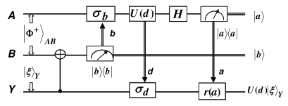
Figure 1: Quantum circuit of the simplified HPV protocol, where $U(d)$ is a quantum operation to be remotely implemented and it is diagonal or antidiagonal, $H$ is a Hadamard gate, $\sigma_{b},\sigma_{d}$ are identity matrices or not gates ($\sigma_{1}$) with respect to $b,d=0$ or $b,d=1$, respectively, and $r(a)=(1-a)\sigma_{0}+a\sigma_{3}$ is an identity matrix when $a=0$ or a phase gate ($\sigma_{3}$) when $a=1$. The measurements $\left|{a}\right\rangle$$\left\langle{a}\right|$ and $\left|{b}\right\rangle$$\left\langle{b}\right|$ are carried out in the computational basis ($a,b=0,1$). “$\Rightarrow$” (crewel with an arrow) indicates the transmission of classical communication to the location of the arrow direction.

III Restricted sets of quantum operations

We have described the simplified HPV protocol of remote implementations of one qubit quantum operations in detail. For our purpose to extend it to the cases of multiqubits, we first seek for the restricted sets of multiqubit quantum operations that can be remotely implemented in a faithful and determined way. Here, through analyzing and discussing the cases of one- and two-qubit operations, we can exhibit our method to obtain the general and explicit forms of restricted sets of multiqubit quantum operations.

Let us start with the analysis of HPV protocol for one qubit. From our point of view, the purpose of Bob’s preparation is to lead to the first qubit (locally acted qubit in Alice’s subsystem) being correlated with the third qubit (remotely operated or controlled qubit in Bob’s subsystem) in such a superposition that for its every orthogonal component state, the first qubit and the third qubit are always located at the same computational bases. Bob arrives at this aim with two possible ways via quantum entanglement resource between the first qubit and the second qubit (in Bob’s subsystem). When Bob uses $b=0$, then this aim has been achieved at, but if Bob takes $b=1$, Alice has to supplement a $\sigma_{1}$ transformation for this aim. It is clear that such a superposition state has at most two orthogonal component states that is equal to the dimension of Hilbert’s space of an unknown state. This implies that we can, at most, transfer two unknown complex numbers from the first qubit to the third qubit. We think that this is a really physical reason why we can only remotely implement a quantum operation belongings to the restricted sets. Without using additional correlation (entanglement), we cannot change this physical fact. However, using additional entanglement will destroy our attempt to save quantum resources.

In the second step, the communication from Bob to Alice is to tell Alice which preparing way Bob has used. In order to include all contributions of operation on the first qubit and transfer them to the third qubit, we need a Hadamard gate acting on the transformed qubit so that Alice’s project measurement on a given computational basis does not lead to losing the actions on the other computational bases, because the first qubit and the third qubit are correlated in the above way. However, the action of the Hadamard gate will result in an algebraic addition of all of matrix elements in some row or column of this operation arising in front of some computation bases. Its advantage is that we are able to transfer the whole effect of operation to the third qubit, but its disadvantage is that we are not able to redivide the algebraic addition of matrix elements in some row or column of this operation because these elements are unknown. A uniquely choice way is to set only one nonzero element in every row or every column of this operation. In fact, this choice is also optimal since it allows the maximal numbers that can be transferred and also includes the unitary operations with such forms. This requirement yields the limitations to the structures of operations that can be remotely implemented, that is, so-called restricted sets of quantum operations. In the case of one qubit, it is easy to see that two restricted sets of quantum operations are made from a kind of diagonal operation and a kind of antidiagonal operation.

For the cases of two qubits, the above analyses are still feasible and valid. Because the unique nonzero element in the first row has four possible positions, the unique nonzero element in the second row has three possible positions, the unique nonzero element in the third row has two possible positions, and the unique nonzero element in the fourth row has one possible position, the restricted sets of operations are made of $4!=24$ kinds of operations.

It is easy to write the set of all of permutations for the list $\{1,2,3,4\}$,

$$\mathbb{P}_{4} = \{(1,2,3,4),(1,2,4,3),(1,3,2,4),(1,3,4,2),(1,4,2,3),(1,4,3,2),$$ (14)

$$(2,1,3,4),(2,1,4,3),(2,3,1,4),(2,3,4,1),(2,4,1,3),(2,4,3,1),$$

$$(3,1,2,4),(3,1,4,2),(3,2,1,4),(3,2,4,1),(3,4,1,2),(3,4,2,1),$$

$$(4,1,2,3),(4,1,3,2),(4,2,1,3),(4,2,3,1),(4,3,1,2),(4,3,2,1)\}.$$

Denoting the $x$th element in this set by

$$p(x)=(p_{1}(x),p_{2}(x),p_{3}(x),p_{4}(x)),$$ (15)

for example $p(1)=(1,2,3,4),p(2)=(1,2,4,3)$, and so on, we can obtain 24 restricted sets of two-qubit operations as follows:

$$T_{2}^{r}(x,t)=\sum_{m=1}^{4}t_{m}\mbox{$\left|{m,D}\right\rangle$}\mbox{$\left\langle{p_{m}(x),D}\right|$},$$ (16)

where we have defined $\mbox{$\left|{1,D}\right\rangle$}=\mbox{$\left|{00}\right\rangle$},\mbox{$\left|{2,D}\right\rangle$}=\mbox{$\left|{01}\right\rangle$},\mbox{$\left|{3,D}\right\rangle$}=\mbox{$\left|{10}\right\rangle$},\mbox{$\left|{4,D}\right\rangle$}=\mbox{$\left|{11}\right\rangle$}$. Here, the label $D$ indicates the decimal system.

It is easy to verify that

$$T_{2}^{r}(x,t)[T_{2}^{r}(x,t)]^{\dagger} = \sum_{m=1}^{4}t_{m}t_{m}^{*}\mbox{$\left|{m,D}\right\rangle$}\mbox{$\left\langle{m,D}\right|$}$$ (17)

$$\left[T_{2}^{r}(x)\right]^{\dagger}T_{2}^{r}(x) = \sum_{m=1}^{4}t_{i}t_{m}^{*}\mbox{$\left|{p_{m}(x),D}\right\rangle$}\mbox{$\left\langle{p_{m}(x),D}\right|$}.$$ (18)

Therefore, in terms of the requirement of the unitary condition for quantum operations, the only nonzero element $t_{m}$ in the $m$th row of quantum operations belonging to the restricted sets should be taken as ${\rm e}^{{\rm i}\phi_{m}}$, and $\phi_{m}$ is real.

The above analyses and discussions have provided evidence of unique forms of restricted sets of two-qubit operations in a kind of protocol of RIO such as ours. In fact, this kind of protocol uses the Hadamard gates to transfer the whole effect of operation to the different qubits, but does not use the extra correlation doing it. Therefore, the forms of restricted sets are uniquely determined. Otherwise, the operation cannot be remotely implemented by using such a kind of protocol.

To remotely implement quantum operations belonging to the above restricted sets, Bob needs a mapping table that provides one-to-one mapping from a classical information $x$ $(x=1,2\cdots,24)$ to a part of his recovery operation $R_{2}(x)$ defined by

$${R}_{2}(x)=T_{2}^{r}(x,0)=\sum_{m=1}^{4}\mbox{$\left|{m,D}\right\rangle$}\mbox{$\left\langle{p_{m}(z),D}\right|$}.$$ (19)

Obviously, it has the same structure as $T_{2}^{r}(x,t)$ to be remotely implemented.

It is easy to see that the controlled kinds of operations

$$U_{C}(1)=\left.T_{2}^{r}(2,t)\right|_{t_{1}=t_{2}=1}=\begin{pmatrix}1&0\\ 0&0\end{pmatrix}\otimes\begin{pmatrix}1&0\\ 0&1\end{pmatrix}+\begin{pmatrix}0&0\\ 0&1\end{pmatrix}\otimes\begin{pmatrix}0&t_{3}\\ t_{4}&0\end{pmatrix}$$ (20)

$$U_{C}(2)=\left.T_{2}^{r}(6,t)\right|_{t_{1}=t_{3}=1}=\begin{pmatrix}1&0\\ 0&1\end{pmatrix}\otimes\begin{pmatrix}1&0\\ 0&0\end{pmatrix}+\begin{pmatrix}0&t_{2}\\ t_{4}&0\end{pmatrix}\otimes\begin{pmatrix}0&0\\ 0&1\end{pmatrix}$$ (21)

$$U_{C}(3)=\left.T_{2}^{r}(7,t)\right|_{t_{1}=t_{2}=1}=\begin{pmatrix}1&0\\ 0&0\end{pmatrix}\otimes\begin{pmatrix}0&t_{3}\\ t_{4}&0\end{pmatrix}+\begin{pmatrix}0&0\\ 0&1\end{pmatrix}\otimes\begin{pmatrix}1&0\\ 0&1\end{pmatrix}$$ (22)

$$U_{C}(4)=\left.T_{2}^{r}(15,t)\right|_{t_{2}=t_{4}=1}=\begin{pmatrix}0&t_{1}\\ t_{3}&0\end{pmatrix}\otimes\begin{pmatrix}1&0\\ 0&0\end{pmatrix}+\begin{pmatrix}1&0\\ 0&1\end{pmatrix}\otimes\begin{pmatrix}0&0\\ 0&1\end{pmatrix}$$ (23)

belong to the restricted set. They are important operations in quantum information processing.

Based on the same reasons stated above, any restricted set of $N$-qubit operations has such a structure that every row and every column of its operations only has one nonzero element, and we denote this nonzero element in the $m$th row by $t_{m}$, that is, the members of $2^{N}!$ restricted sets of $N$-qubit operations have the forms

$$T^{r}_{N}(x,t)=\sum_{m=1}^{2^{N}}t_{m}\mbox{$\left|{m,D}\right\rangle$}\mbox{$\left\langle{p_{m}(x),D}\right|$},$$ (24)

where $x=1,2,\cdots,2^{N}!$ and

$$p(x)=(p_{1}(x),p_{2}(x),\cdots,p_{2^{N}}(x))$$ (25)

is an element belonging to the set of all permutations for the list $\{1,2,\cdots,2^{N}\}$. All of the restricted sets of $N$-qubit operations are denoted by $\mathbb{T}^{r}_{N}$.

For the cases of $N$-qubit operations, we can take all nonzero elements of $T^{r}_{N}(x,t)$ as $1$ and obtain its fixed form $R_{N}(x)$, that is

$${R}_{N}(x)=T^{r}_{N}(x,0)=\sum_{m=1}^{2^{N}}\mbox{$\left|{m,D}\right\rangle$}\mbox{$\left\langle{p_{m}(x),D}\right|$}.$$ (26)

It will be used in Bob’s recovery operation of our protocol.

It must be emphasized that we usually study the cases in which $T^{r}_{N}(x,t)$ is unitary, although it does not affect our protocol. Before the beginning of the protocol, we need to build two mapping tables: one provides one-to-one mapping from $T^{r}_{N}(x,t)\in\mathbb{T}^{r}_{N}$ to the classical information $x$ which is known by Alice and another provides one-to-one mapping from a classical information $x$ to $R_{N}(x)$ which is known by Bob.

It is clear that our explicit restricted sets of multiqubit operations are not reducible to the simple direct product of two restricted sets of one qubit operations. Thus, in this sense, our protocol can be thought of as a development of HPV protocol to the cases of multiqubits.

IV Protocol in the case of two qubits

Now let us propose the protocol of remote implementations of two-qubit quantum operations belonging to 24 restricted sets in detail.

Assume the initial state of the joint system to be

$$\mbox{$\left|{\Psi_{A_{1}B_{1}A_{2}B_{2}Y_{1}Y_{2}}^{\rm ini}}\right\rangle$}=\mbox{$\left|{\Phi^{+}}\right\rangle$}_{A_{1}B_{1}}\otimes\mbox{$\left|{\Phi^{+}}\right\rangle$}_{A_{2}B_{2}}\mbox{$\left|{\xi}\right\rangle$}_{Y_{1}Y_{2}},$$ (27)

where the unknown state of two qubits is

$$\mbox{$\left|{\xi}\right\rangle$}_{Y_{1}Y_{2}}=\sum_{j_{1},j_{2}=0}^{1}y_{j_{1}j_{2}}\mbox{$\left|{j_{1}j_{2}}\right\rangle$}_{Y_{1}Y_{2}},$$ (28)

the qubits $A_{1},A_{2}$ belong to Alice, the other four qubits $B_{1},B_{2},Y_{1},Y_{2}$ are owned by Bob. It is clear that Alice and Bob share initially two Bell states.

Note that the Hilbert space of the joint system is initially taken as a series of direct products of Hilbert spaces of all qubits according to the following sequence:

$$H=H_{A_{1}}\otimes H_{B_{1}}\otimes H_{A_{2}}\otimes H_{B_{2}}\otimes H_{Y_{1}}\otimes H_{Y_{2}}.$$ (29)

We can simply call this sequence “space structure” and denote it by a bit-string; for example, the space structure of the above Hilbert space is $A_{1}B_{1}A_{2}B_{2}Y_{1}Y_{2}$. Obviously, taking such a space structure, the subspace belonging to Alice or Bob is separated. It will lead to inconvenience in the expression of local operations acting on their full subspaces and in the proof of the protocol of multiqubits. Therefore, there is a need to change the space structure. This can be realized by a series of swapping transformations, which are studied in Appendix A.

In terms of the general swapping transformations defined in Appendix A, we can change the initial space structure, for example,

$$\mbox{$\left|{a_{1}b_{1}a_{2}b_{2}y_{1}y_{2}}\right\rangle$}_{A_{1}B_{1}A_{2}B_{2}Y_{1}Y_{2}} = \Upsilon^{-1}(3,2)\left(\mbox{$\left|{a_{1}b_{1}y_{1}}\right\rangle$}_{A_{1}B_{1}Y_{1}}\otimes\mbox{$\left|{a_{2}b_{2}y_{2}}\right\rangle$}_{A_{2}B_{2}Y_{2}}\right)$$ (30)

$$\mbox{$\left|{a_{1}b_{1}a_{2}b_{2}y_{1}y_{2}}\right\rangle$}_{A_{1}B_{1}A_{2}B_{2}Y_{1}Y_{2}} = \left[\Lambda^{-1}(2,2)\otimes I_{4}\right]\left(\mbox{$\left|{a_{1}a_{2}}\right\rangle$}_{A_{1}A_{2}}\otimes\mbox{$\left|{b_{1}b_{2}}\right\rangle$}_{B_{1}B_{2}}\otimes\mbox{$\left|{y_{1}y_{2}}\right\rangle$}_{Y_{1}Y_{2}}\right)$$ (31)

$$\mbox{$\left|{a_{1}b_{1}a_{2}b_{2}y_{1}y_{2}}\right\rangle$}_{A_{1}B_{1}A_{2}B_{2}Y_{1}Y_{2}} = \Gamma^{-1}(3,2)\left(\mbox{$\left|{a_{1}a_{2}}\right\rangle$}_{A_{1}A_{2}}\otimes\mbox{$\left|{y_{1}y_{2}}\right\rangle$}_{Y_{1}Y_{2}}\otimes\mbox{$\left|{b_{1}b_{2}}\right\rangle$}_{B_{1}B_{2}}\right).$$ (32)

Thus, we can express our formula compactly and clearly in the whole space, and can finally prove our protocol conveniently and strictly. Our notations in the whole space will be helpful for in understanding the problems even if a little complication in expressions is induced. It will be seen that such notations are more useful for the extension to the cases of multiqubits. However, it must be emphasized that these swapping transformations in the following formula do not really exist in the practical process.

Step One: Bob’s preparation. Our protocol begins from this step. Bob first performs two controlled-not using, respectively, his qubits $Y_{1}$ and $Y_{2}$ as two control qubits, $B_{1}$ and $B_{2}$ as two target qubits, and then measures his two qubits $B_{1}$ and $B_{2}$ in the computational basis $\mbox{$\left|{b_{1}}\right\rangle$}_{B_{1}}\mbox{$\left\langle{b_{1}}\right|$}\otimes\mbox{$\left|{b_{2}}\right\rangle$}_{B_{2}}\mbox{$\left\langle{b_{2}}\right|$}$ $(b_{1},b_{2}=0,1)$. Therefore, Bob’s preparation reads

$${\mathcal{P}}_{B}(b_{1},b_{2})=\Upsilon^{-1}(3,2)\left\{\bigotimes_{m=1}^{2}\sigma_{0}^{A_{m}}\otimes\left[\left(\mbox{$\left|{b_{m}}\right\rangle$}_{B_{m}}\mbox{$\left\langle{b_{m}}\right|$}\otimes\sigma_{0}^{Y_{m}}\right)C^{\rm not}(0,1)\right]\right\}\Upsilon(3,2),$$ (33)

where $\Upsilon(3,N)$ is defined in Appendix A. Note that this expression is written in the whole joint system so that we can prove our protocol more conveniently in Appendix B.

If we do not use the swapping transformations, the form of Bob’s preparation becomes

$${\mathcal{P}}_{B}(b_{1},b_{2}) = \left(\sigma_{0}^{A_{1}}\otimes\mbox{$\left|{b_{1}}\right\rangle$}_{B_{1}}\mbox{$\left\langle{b_{1}}\right|$}\otimes\sigma_{0}^{A_{2}}\otimes\mbox{$\left|{b_{2}}\right\rangle$}_{B_{2}}\mbox{$\left\langle{b_{2}}\right|$}\otimes\sigma_{0}^{Y_{1}}\otimes\sigma_{0}^{Y_{2}}\right)\cdot\left(\sigma_{0}^{A_{1}}\otimes C^{\rm not}_{2}(0,1)\otimes\sigma_{0}^{Y_{2}}\right)$$ (34)

$$\times\left(\sigma_{0}^{A_{1}}\otimes\sigma_{0}^{B_{1}}\otimes\sigma_{0}^{A_{2}}\otimes C_{1}^{\rm not}(0,1)\right).$$

Here, $C_{M}^{\rm not}$ can be called the separated controlled-not since its control and target are separated by $M$ qubits, that is, its definition is

$$C^{\rm not}_{M}(0,1)=\sigma_{0}\otimes\left(\bigotimes_{m=1}^{M}\sigma_{0}\right)\otimes\left(\mbox{$\left|{0}\right\rangle$}\mbox{$\left\langle{0}\right|$}\right)+\sigma_{1}\otimes\left(\bigotimes_{m=1}^{M}\sigma_{0}\right)\otimes\left(\mbox{$\left|{1}\right\rangle$}\mbox{$\left\langle{1}\right|$}\right),$$ (35)

while $(0,1)$ indicates that the last qubit is a control and the first qubit is a target and is flipped when the control qubit is $\left|{1}\right\rangle$. If $M=0$, it comes back to the usual controlled-not. It is clear that using the general swapping transformations can simplify the expressions of formula in form.

Step Two: Classical communication from Bob to Alice. After finishing his measurement on the computational basis, Bob transfers two classical bits $b_{1},b_{2}$ to Alice. This step is necessary so that Alice can determine her sending operations.

It must be emphasized that Bob’s preparation step has four equivalent ways corresponding to, respectively, $b_{1}b_{2}$ taking $00,01,10,11$ in order to carry out the protocol. If Bob first fixes the value of $b_{1}b_{2}$ and tells Alice before the beginning of the protocol, this step can be saved. In particular, when $b_{1}b_{2}$ is just taken as $00$, Alice also does not need the transformation $\sigma_{b_{1}}\otimes\sigma_{b_{2}}$ in the next step, since $\sigma_{0}\otimes\sigma_{0}$ is trivial.

Step Three: Alice’s sending. After receiving Bob’s classical bits $b_{1}b_{2}$, Alice, on her two qubits (the qubits $A_{1}A_{2}$), first performs $\sigma_{b_{1}}^{A_{1}}\otimes\sigma_{b_{2}}^{A_{2}}$, secondly acts $T_{2}^{r}(x,t)$ to be remotely implemented, then carries out two Hadamard transformations, and finally measures her two qubits in the computational basis $\mbox{$\left|{a_{1}}\right\rangle$}_{A_{1}}\mbox{$\left\langle{a_{1}}\right|$}\otimes\mbox{$\left|{a_{2}}\right\rangle$}_{A_{2}}\mbox{$\left\langle{a_{2}}\right|$}$ $(a_{1},a_{2}=0,1)$. Since the basis vector of Alice’s space has the structure $\mbox{$\left|{a_{1}a_{2}}\right\rangle$}_{A_{1}A_{2}}$, all of Alice’s local operations and measurement are just

$${\mathcal{S}}_{A}(a_{1},b_{1},a_{2},b_{2};x,t) = \left[\Lambda^{-1}(2,2)\otimes I_{4}\right]\left\{\left[\left(\mbox{$\left|{a_{1}a_{2}}\right\rangle$}_{A_{1}A_{2}}\mbox{$\left\langle{a_{1}a_{2}}\right|$}\right)\left(H^{A_{1}}\otimes H^{A_{2}}\right)\right.\right.$$ (36)

$$\left.\left.\times T_{2}^{r}(x,t)\left(\sigma_{b_{1}}^{A_{1}}\otimes\sigma_{b_{2}}^{A_{2}}\right)\right]\otimes I_{16}\right\}\left[\Lambda(2,2)\otimes I_{4}\right],$$

where $\Lambda(2,2)$ is defined in Appendix A and $I_{m}$ is a $m$ dimensional identity matrix.

Step Four: Classical communication from Alice to Bob. After finishing her measurement on the computational basis $\mbox{$\left|{a_{1}}\right\rangle$}_{A_{1}}\mbox{$\left\langle{a_{1}}\right|$}\otimes\mbox{$\left|{a_{2}}\right\rangle$}_{A_{2}}\mbox{$\left\langle{a_{2}}\right|$}$ $(a_{1},a_{2}=0,1)$, Alice transfers two classical bits $a_{1},a_{2}$ to Bob. Moreover, Alice also needs to transfer $x$ (which can be encoded by five classical bits) to Bob in order to let him know the transferred operation $T_{2}^{r}(x,t)$ belonging to which restricted set, unless they prescribed the transferred operation $T_{2}^{r}(x,t)$ belonging to a given restricted set before the beginning of the protocol. All of the classical information is necessary for Bob so that he can determine his recovery operations.

Step Five: Bob’s recovery. In order to obtain the remote implementations of quantum operations in a faithful and determined way, Bob performs his recovery operation,

$${\mathcal{R}}_{B}(a_{1},a_{2};x)=I_{16}\otimes\left\{\left[\mathfrak{r}^{Y_{1}}(a_{1})\otimes\mathfrak{r}^{Y_{2}}(a_{2})\right]\cdot{R}_{2}(x)\right\},$$ (37)

where $\mathfrak{r}(y)$ is defined by

$$\mathfrak{r}(y)=(1-y)\sigma_{0}+y\sigma_{3},$$ (38)

while $R_{2}(x)$ is obtained by the mapping table from the classical information $x$ to $R_{2}(x)$. For example, Bob receives $1$ (which can be encoded by $00000$), thus he knows $R(1)$ is an identity matrix; Bob receives $2$ (which can be encoded by $00001$), thus he knows

$$R_{2}(2)=\left(\begin{array}[]{cccc}1&0&0&0\\ 0&1&0&0\\ 0&0&0&1\\ 0&0&1&0\end{array}\right),$$ (39)

and so on. The mapping between $x$ and $R_{2}(x)$ is given in advance before the beginning of the protocol.

Finally, all of the operations including measurements in the whole space for the remote implementations of quantum operations of two qubit can be written jointly as

$${\mathcal{I}}_{R}(a_{1},b_{1},a_{2},b_{2};x,t)={\mathcal{R}}_{B}(a_{1},a_{2};x)\cdot{\mathcal{S}}_{A}(a_{1},b_{1},a_{2},b_{2};x,t)\cdot{\mathcal{P}}_{B}(b_{1},b_{2}).$$ (40)

Its action on the initial state gives the remote implementations of two qubit quantum operations belonging to the above 24 restricted sets, that is, the final state becomes

$$\left|{\Psi_{A_{1}B_{1}A_{2}B_{2}Y_{1}Y_{2}}^{\rm final}(a_{1},b_{1},a_{2},b_{2};x,t)}\right\rangle = {\mathcal{I}}_{R}(a_{1},b_{1},a_{2},b_{2};x)\mbox{$\left|{\Psi_{A_{1}B_{1}A_{2}B_{2}Y_{1}Y_{2}}^{\rm ini}}\right\rangle$}$$ (41)

$$= \frac{1}{4}\mbox{$\left|{a_{1}b_{1}a_{2}b_{2}}\right\rangle$}_{A_{1}B_{1}A_{2}B_{2}}\otimes T_{2}^{r}(x,t)\mbox{$\left|{\xi}\right\rangle$}_{Y_{1}Y_{2}},$$ (42)

where $a_{m},b_{n}=0,1$; $m,n=1,2$. Therefore, our protocol completes faithfully and determinedly the remote implementations of quantum operations $T_{2}^{r}(x,t)$ belonging to 24 restricted sets. Its proof is found in Appendix B when $N=2$.

V Extension to the cases of $N$ qubits

Based on our above protocol of remote implementations of two-qubit operations belonging to our restricted sets, we can extend it to the cases of more than two qubits without obvious difficulty. Our protocol consists of five steps for the remote implementations of $N$-qubit operations belonging to our restricted sets. Set the initial state as

$$\mbox{$\left|{\Psi_{N}^{\rm ini}}\right\rangle$}=\left(\bigotimes_{m=1}^{N}\mbox{$\left|{\Phi^{+}}\right\rangle$}_{A_{m}B_{m}}\right)\otimes\mbox{$\left|{\xi}\right\rangle$}_{Y_{1}Y_{2}\cdots Y_{N}},$$ (43)

where $\mbox{$\left|{\xi}\right\rangle$}_{Y_{1}Y_{2}\cdots Y_{N}}$ is an arbitrary (unknown) pure state in an $N$-qubit system, that is

$$\mbox{$\left|{\xi}\right\rangle$}_{Y_{1}Y_{2}\cdots Y_{N}}=\sum_{k_{1},k_{2},\cdots k_{N}=0}^{1}y_{k_{1}k_{2}\cdots k_{N}}\mbox{$\left|{k_{1}k_{2}\cdots k_{N}}\right\rangle$}.$$ (44)

It is clear that the space structure is initially

$$\prod_{m=1}^{N}(A_{m}B_{m})\prod_{n=1}^{N}Y_{n}.$$ (45)

Usually, in order to avoid possible errors and provide convenience in the proof, we need to set the sequential structure of direct product space of qubits, or a sequence of direct products of qubit-space basis vectors in the multiqubit systems. For Alice’s space, we set its sequential structure as $A_{1}A_{2}\cdots A_{N}$, in other words, its basis vector has the form $\mbox{$\left|{a_{1}}\right\rangle$}_{A_{1}}\mbox{$\left|{a_{2}}\right\rangle$}_{A_{2}}\cdots\mbox{$\left|{a_{N}}\right\rangle$}_{A_{N}}$ (or $\mbox{$\left|{a_{1}a_{2}\cdots a_{N}}\right\rangle$}_{A_{1}A_{2}\cdots A_{N}}$). Similarly, we set the sequential structure of Bob’s space as $B_{1}B_{2}\cdots B_{N}Y_{1}Y_{2}\cdots Y_{N}$, in other words, its basis vector has the form $\mbox{$\left|{b_{1}}\right\rangle$}_{B_{1}}\mbox{$\left|{b_{2}}\right\rangle$}_{B_{2}}\cdots\mbox{$\left|{b_{N}}\right\rangle$}_{B_{N}}\mbox{$\left|{y_{1}}\right\rangle$}_{Y_{1}}\mbox{$\left|{y_{2}}\right\rangle$}_{Y_{2}}\cdots\mbox{$\left|{y_{N}}\right\rangle$}_{Y_{N}}$. It is clear that for an $N$-qubit system, its space structure can be represented by a bit-string with the length of $N$.

Now, let us describe our protocol in a concise way.

Step One: Bob’s preparation

$${\mathcal{P}}_{B}(b_{1},b_{2},\cdots,b_{N})=\Upsilon^{-1}(3,N)\left\{\bigotimes_{m=1}^{N}\sigma_{0}^{A_{m}}\otimes\left[\left(\mbox{$\left|{b_{m}}\right\rangle$}\mbox{$\left\langle{b_{m}}\right|$}\otimes\sigma_{0}\right)C^{\rm not}(0,1)\right]\right\}\Upsilon_{N}(3,N),$$ (46)

where $\Upsilon(3,N)$ is defined in Appendix A. It must be emphasized that $\Upsilon(3,N)$ does not appear in the practical process, it is only required to express our steps clearly and compactly.

Step Two: Classical Communication from Bob to Alice. Alice transfers a classical bit-string $b_{1}b_{2}\cdots b_{N}$ to Bob unless Bob and Alice have an arrangement about Bob’s preparing method (that is $b_{1}b_{2}\cdots b_{N}$ to be determined by Bob and known by Alice) before the beginning of the protocol.

Step Three: Alice’s sending.

$${\mathcal{S}}_{A}(a_{1},b_{1},a_{2},b_{2},\cdots,a_{N},b_{N};x,t) = \left(\Lambda^{-1}(2,N)\otimes I_{2^{N}}\right)\left[\left(\bigotimes_{m=1}^{N}\mbox{$\left|{a_{m}}\right\rangle$}_{A_{m}}\mbox{$\left\langle{a_{m}}\right|$}\right)\cdot\left(\bigotimes_{m=1}^{N}H^{A_{m}}\right)\right.$$ (47)

$$\left.\cdot T^{r}_{N}(x,t)\cdot\left(\bigotimes_{m=1}^{N}\sigma_{b_{m}}^{A_{m}}\right)\otimes I_{4^{N}}\right]\left(\Lambda(2,N)\otimes I_{2^{N}}\right),$$

where $\Lambda_{N}(2,N)$ is defined in Appendix A.

Step Four: Classical Communication from Alice to Bob. Alice transfers a classical bit-string $a_{1}a_{2}\cdots a_{N}$ and a classical information $x$ (which can be encoded by $\left[\log_{2}(2^{N}!)\right]+1$ $c$-bit string, where $[\cdots]$ means taking the integer part) corresponding to the quantum operation $T^{r}_{N}(x,t)$ to be remotely implemented in her mapping table.

Step Five: Bob’s recovery.

$${\mathcal{R}}_{B}(a_{1},a_{2}\cdots a_{N};x)=I_{4^{N}}\otimes\left\{\!\!\left(\bigotimes_{m=1}^{N}\mathfrak{r}(a_{m})\right)\cdot{R}_{N}(x)\right\},$$ (48)

where $R_{N}(x)$ is determined by Bob’s mapping table.

Thus, all of the operations including measurements in the extension of remote implementations of quantum operations to the case of $N$ qubits can be written as

$${\mathcal{I}}_{R}(a_{1},b_{1},a_{2},b_{2};\cdots,a_{N},b_{N};x,t) = {\mathcal{R}}_{B}(a_{1},a_{2},\cdots a_{N};x)$$ (49)

$$\times{\mathcal{S}}_{A}(a_{1},b_{1},a_{2},b_{2},\cdots,a_{N},b_{N};x,t)$$

$$\times{\mathcal{P}}_{B}(b_{1},b_{2},\cdots,b_{N}).$$

The final state becomes

$$\left|{\Psi_{N}^{\rm final}(a_{1},b_{1},a_{2},b_{2},\cdots,a_{N},b_{N};x)}\right\rangle$$

$$\quad={\mathcal{I}}_{R}(a_{1},b_{1},a_{2},b_{2};\cdots,a_{N},b_{N};x,t)\mbox{$\left|{\Psi_{N}^{\rm ini}}\right\rangle$}$$ (50)

$$\quad=\frac{1}{2^{N}}\left(\bigotimes_{i=1}^{N}\mbox{$\left|{a_{i}b_{i}}\right\rangle$}_{A_{i}B_{i}}\right)\otimes T^{r}_{N}(x,t)\mbox{$\left|{\xi}\right\rangle$}_{Y_{1}Y_{2}\cdots Y_{N}}.$$ (51)

where $a_{m},b_{n}=0,1$; $m,n=1,2,\cdots,N$.

It is easy to see that our restricted sets of three-qubit operations include the interesting controlled-controlled-$U(d)$ gate with the form

$$U^{\rm cc}(d)=\left(\mbox{$\left|{00}\right\rangle$}\mbox{$\left\langle{00}\right|$}+\mbox{$\left|{01}\right\rangle$}\mbox{$\left\langle{01}\right|$}+\mbox{$\left|{10}\right\rangle$}\mbox{$\left\langle{10}\right|$}\right)\otimes\sigma_{0}+\mbox{$\left|{11}\right\rangle$}\mbox{$\left\langle{11}\right|$}\otimes U(d),$$ (52)

where $U(d)$ is a diagonal or antidiagonal operation of one-qubit systems. Just as well-known, it, together with the operations (20-23), can be used to construct a universal gate.

The protocol proof of remote implementations of $N$-qubit operations belonging to our restricted sets is given in Appendix B.

VI Discussion and conclusion

In summary, we propose and prove the protocol of remote implementations of partially unknown quantum operations of multiqubits belonging to the restricted sets, and we obtain the general and explicit forms of these restricted sets, that is, every row and every column of an arbitrary member of operations belonging to the restricted sets only has one nonzero element. Our protocol is based on the simplified HPV scheme, but it can be thought of as a development of HPV scheme to the cases of multiqubit systems since our restricted sets of multiqubit operations are not simply reducible to the direct products of HPV restricted sets of one-qubit operations. Moreover, we have given evidence of the uniqueness and optimization of our restricted sets based on the precondition that our protocol only uses $N$ Bell’s pairs. In order to show our protocol in the above several aspects, we investigate in detail the cases of two qubits. Note that those quantum operations with the clearly physical significance and practical applications are included in our restricted sets which can be remotely implemented. It should be pointed out that the universal recovery operations found by us are useful because they will be helpful for the design of unified recovery quantum circuits in the near future. This implies that the quantum operations that can be remotely implemented are extended from only belonging to a given restricted set to belonging to all of the restricted sets in our protocol. Its advantages is obviously that the power of remote implementations of quantum operations is enhanced. Of course, the unified recovery operations need two mapping tables that are known, respectively, by Alice and Bob before the beginning of the protocol.

In the area of resource consumption, the remote implementations of quantum operations belonging to two restricted sets of one-qubit operations need one $e$-bit which is shared by the sender and receiver and three $c$-bits (or two when Bob fixes his preparing way) from which one $c$-bit is transferred from the receiver to the sender and two $c$-bits are transferred from the sender to the receiver. In our protocol, we can see that the remote implementations of quantum operations belonging to 24 restricted sets of two-qubit operations need two $e$-bits and nine $c$-bits (or seven $c$-bits when Bob fixes his preparing way), where two $e$-bits are shared by the sender and the receiver, respectively, and two of nine $c$-bits are transferred from the receiver to the sender while the other seven $c$-bits are transferred from the sender to the receiver. For the case of $N$ qubit operations, since the number of restricted sets that can be remotely implemented is $2^{N}!$, their remote implementations need $N$ $e$-bits and $2N+[\ln_{2}(2^{N}!)]+1$ $c$-bits (or $N+[\ln_{2}(2^{N}!)]+1$ $c$-bits when Bob fixes his preparing way), where $N$ $e$-bits are shared by the sender and the receiver, and $N$ $c$-bits are transferred from the receiver to the sender while the other $N+[\ln_{2}(2^{N}!)]+1$ $c$-bits are transferred from the sender to the receiver. Here, “$[x]$” means taking the integer part of $x$. In addition, the fixed local operations $R_{N}(x)$ need to be used, and two mapping tables from $T^{r}_{N}(x,t)$ to a classical information $x$ and from a classical information $x$ to $R_{N}(x)$ need to be built before the beginning of the protocol. Usually, the number of interesting restricted sets that can be remotely implemented may be small, and the classical resource can be correspondingly decreased. However, this will pay the price that the power of protocol of remote implementations of quantum operations is reduced. It should be pointed out that the implementations of nonlocal quantum operations are different from the remote implementations of the quantum operations. Therefore, the resource used by them may be different in general.

Similar to the conclusion provided by Refs. Huelga1 ; Huelga2 , we have not found a faithful scheme without using the maximum entanglement Our1 . Actually, this is partially because there is no obvious physical significance when a unitary operation belonging to the restricted sets acts on a density matrix of diagonal state, and such an action is equivalent to the known one that will be used in the recovery operation. For example, a phase gate on one qubit acting on a density matrix of a diagonal state gives nothing, an antidiagonal unitary transformation on one qubit acting on a density matrix of a diagonal state is just a flip gate. Of course, the study on the possible tradeoffs between the entanglement and classical communication will still be important in the near future.

Furthermore, we can investigate the controlled remote implementations of partially unknown quantum operations belonging to the restricted sets of one- and multiqubits. Similar to the controlled teleportation of a quantum state via the GHZ states, the controlled remote implementations of partially unknown quantum operations can use the GHZ states which are a very important quantum information resource GHZ . In our view, the controlled remote implementations of quantum operations should have some remarkable applications in the remote quantum information processing and communication including the future quantum internet. Here, a quantum internet is a counterpart to the classical one, but it connects some quantum computers that are located at different places together and is used for the remote communication of quantum information and remote implementations of quantum operations. The relevant conclusions are studied in OurCCRIO .

Appendix A Swapping transformation

Here, we study the general swapping transformations, which are combinations of a series of usual swapping transformations. They are used in our protocol in order to express our formula clearly and compactly, and prove our protocol easily and strictly.

Note that a swapping transformation of two neighbor qubits ($2\times 2$ matrix) is defined by

$$S_{W}=\left(\begin{array}[]{cccc}1&0&0&0\\ 0&0&1&0\\ 0&1&0&0\\ 0&0&0&1\end{array}\right).$$ (53)

Its action is

$$S_{W}\mbox{$\left|{\alpha_{X}\beta_{Y}}\right\rangle$}=\mbox{$\left|{\beta_{Y}\alpha_{X}}\right\rangle$},\quad S_{W}(M^{X}\otimes M^{Y})S_{W}=M^{Y}\otimes M^{X}.$$ (54)

This means that the swapping transformation changes the space structure $H_{X}\otimes H_{Y}$ into $H_{Y}\otimes H_{X}$.

For an $N$-qubit system, the swapping gate of the $i$th qubit and the $i+1$th qubit reads

$$S_{N}(i,i+1)=\sigma_{0}^{\otimes(i-1)}\otimes S_{W}\otimes\sigma_{0}^{\otimes(N-i-1)}.$$ (55)

Two rearranged transformations are defined by

$$F_{N}(i,j)=\prod_{\alpha=1\leftarrow}^{j-i}S_{N}(j-\alpha,j+1-\alpha)$$ (56)

$$P_{N}(j,k)=\prod_{\beta=j\leftarrow}^{k-1}S_{N}(\beta,\beta+1)$$ (57)

where $F_{N}(i,j)$ extracts out the spin-state of site $j$, and rearranges it forwards to the site $i$ ($i<j$) in the qubit-string, where $P_{N}(j,k)$ extracts out the spin-state of site $j$, and rearranges it backwards to the site $k$ ($k>j$) in the qubit-string. Note that “$\leftarrow$” means that the factors are arranged from right to left corresponding to $\alpha,\beta$ from small to large. Now, in terms of $P(j,k)$, we can introduce two general swapping transformations with the forms

$${\Lambda}(2,N)=\prod_{i=1\leftarrow}^{N-1}P_{2N}\left(2(N-i),2N-i\right),\quad(N\geq 2)$$ (58)

$${\Omega}(2,N)=\prod_{i=1\leftarrow}^{N}P_{2N}\left(1,2N\right),\quad(N\geq 2)$$ (59)

Thus,

$${\Lambda}(2,N)\left(\bigotimes_{i=1}^{N}\mbox{$\left|{a_{i}b_{i}}\right\rangle$}\right)=\left(\bigotimes_{i=1}^{N}\mbox{$\left|{a_{i}}\right\rangle$}\right)\otimes\left(\bigotimes_{j=1}^{N}\mbox{$\left|{b_{j}}\right\rangle$}\right),$$ (60)

$${\Lambda}(2,N)\left(\bigotimes_{k=1}^{N}\left(M_{\alpha_{i}}^{A_{i}}\otimes M_{\beta_{i}}^{B_{i}}\right)\right){\Lambda}^{-1}(2,N)=\left(\bigotimes_{i=1}^{N}M_{\alpha_{i}}^{A_{i}}\right)\otimes\left(\bigotimes_{j=1}^{N}M_{\beta_{j}}^{B_{j}}\right),$$ (61)

$${\Omega}(2,N)\left[\left(\bigotimes_{i=1}^{N}\mbox{$\left|{a_{i}}\right\rangle$}\right)\otimes\left(\bigotimes_{j=1}^{N}\mbox{$\left|{b_{j}}\right\rangle$}\right)\right]=\left(\bigotimes_{i=1}^{N}\mbox{$\left|{b_{i}}\right\rangle$}\right)\otimes\left(\bigotimes_{j=1}^{N}\mbox{$\left|{a_{j}}\right\rangle$}\right),$$ (62)

$${\Omega}(2,N)\left[\left(\bigotimes_{i=1}^{N}M_{\alpha_{i}}^{A_{i}}\right)\left(\bigotimes_{i=1}^{N}M_{\beta_{i}}^{B_{i}}\right)\right]{\Omega}^{-1}(2,N)=\left(\bigotimes_{i=1}^{N}M_{\beta_{i}}^{B_{i}}\right)\otimes\left(\bigotimes_{j=1}^{N}M_{\alpha_{j}}^{A_{j}}\right).$$ (63)

Similarly, we can introduce

$${\Upsilon}(3,N)=\prod_{i=1\leftarrow}^{N-1}F_{3N}\left(3i,2N+i\right),\quad(N\geq 2).$$ (64)

$$\Gamma(3,N)=\left(I_{2^{N}}\otimes\Omega(2,N)\right)\left(\Lambda(2,N)\otimes I_{2^{N}}\right).$$ (65)

Thus,

$${\Upsilon}(3,N)\left(\bigotimes_{i=1}^{N}\mbox{$\left|{a_{i}b_{i}}\right\rangle$}\right)\otimes\left(\bigotimes_{j=1}^{N}\mbox{$\left|{y_{j}}\right\rangle$}\right)=\bigotimes_{i=1}^{N}\mbox{$\left|{a_{i}b_{i}y_{i}}\right\rangle$},$$ (66)

$${\Upsilon}(3,N)\left[\bigotimes_{k=1}^{N}\left(M_{\alpha_{i}}^{A_{i}}\otimes M_{\beta_{i}}^{B_{i}}\right)\right]\left(\bigotimes_{j=1}^{N}M_{\gamma_{j}}^{Y_{j}}\right){\Upsilon}^{-1}(3,N)=\bigotimes_{i=1}^{N}M_{\alpha_{i}}^{A_{i}}\otimes M_{\beta_{i}}^{B_{i}}\otimes M_{\gamma_{i}}^{Y_{i}},$$ (67)

$${\Gamma}(3,N)\left(\bigotimes_{i=1}^{N}\mbox{$\left|{a_{i}b_{i}}\right\rangle$}\right)\otimes\left(\bigotimes_{j=1}^{N}\mbox{$\left|{y_{j}}\right\rangle$}\right)=\left(\bigotimes_{i=1}^{N}\mbox{$\left|{a_{i}}\right\rangle$}\right)\otimes\left(\bigotimes_{j=1}^{N}\mbox{$\left|{y_{j}}\right\rangle$}\right)\otimes\left(\bigotimes_{k=1}^{N}\mbox{$\left|{b_{k}}\right\rangle$}\right),$$ (68)

$${\Gamma}(3,N)\left[\bigotimes_{k=1}^{N}\left(M_{\alpha_{i}}^{A_{i}}\otimes M_{\beta_{i}}^{B_{i}}\right)\right]\left(\bigotimes_{j=1}^{N}M_{\gamma_{j}}^{Y_{j}}\right){\Gamma}^{-1}(3,N)$$

$$\quad=\left(\bigotimes_{i=1}^{N}M_{\alpha_{i}}^{A_{i}}\right)\otimes\left(\bigotimes_{j=1}^{N}M_{\gamma_{j}}^{Y_{j}}\right)\otimes\left(\bigotimes_{k=1}^{N}M_{\beta_{k}}^{B_{k}}\right).$$ (69)

More generally, consider the set $\mathbb{Q}_{N}$ to be a whole permutation of the bit-string ${a_{1}a_{2}\cdots a_{N}}$, and denote the $z$th element with a bit-string form $Q(z)=q_{1}(z)q_{2}(z)\cdots q_{N}(z)$, we can always obtain such a general swapping transformation $W_{N}$ that a computational basis $\left|{a_{1}a_{2}\cdots a_{N}}\right\rangle$ of $N$-qubit systems can be swapped as another basis $\left|{q_{1}(z)q_{2}(z)\cdots q_{N}(z)}\right\rangle$ in which $q_{1}(z)q_{2}(z)\cdots q_{N}(z)$ is an arbitrary element of $\mathbb{Q}_{N}$. That is, we can write a given general swapping transformation $W_{N}\left[a_{1}a_{2}\cdots a_{N}\rightarrow q_{1}(z)q_{2}(z)\cdots q_{N}(z)\right]$,

$$W_{N}\left[{a_{1}a_{2}\cdots a_{N}}\rightarrow{q_{1}(z)q_{2}(z)\cdots q_{N}(z)}\right]\mbox{$\left|{a_{1}a_{2}\cdots a_{N}}\right\rangle$}=\mbox{$\left|{q_{1}(z)q_{2}(z)\cdots q_{N}(z)}\right\rangle$}.$$ (70)

Furthermore, if we denote two dimensional space $A_{i}$ spanned by $\left|{a_{i}}\right\rangle$ ($a_{i}=0,1$ and $i=1,2,\cdots N$), while $M^{A_{i}}$ is a matrix belonging to this space, we obviously have

$$W_{N}^{-1}\left[{a_{1}a_{2}\cdots a_{N}}\rightarrow{q_{1}(z)q_{2}(z)\cdots q_{N}(z)}\right]\left(\prod_{i=1}^{N}M^{A_{i}}\right)$$

$$W_{N}\left[{a_{1}a_{2}\cdots a_{N}}\rightarrow{q_{1}(z)q_{2}(z)\cdots q_{N}(z)}\right]=\left(\prod_{i=1}^{N}M^{A_{q_{i}(z)}}\right).$$ (71)

Therefore, the general swapping transformation $W_{N}$ defined above can be used to change the space structure of multiqubits systems.

Appendix B Proof of our protocol

Here, we would like to prove our protocol of remote implementations of quantum operations belonging to our restricted sets in the cases with more than one qubit.

By using the swapping transformation $\Upsilon$, we can rewrite the initial state

$$\mbox{$\left|{\Psi^{\rm ini}_{N}}\right\rangle$}=\frac{1}{\sqrt{2^{N}}}\Upsilon^{-1}(3,N)\sum_{k_{1},\cdots k_{N}=0}^{1}y_{k_{1}\cdots k_{N}}\bigotimes_{m=1}^{N}\left(\mbox{$\left|{00k_{m}}\right\rangle$}+\mbox{$\left|{11k_{m}}\right\rangle$}\right).$$ (72)

From Bob’s preparation, it follows that

$$\left|{\Psi^{P}(b_{1},\cdots b_{N})}\right\rangle = \mathcal{P}_{B}(b_{1},b_{2},\cdots,b_{N})\mbox{$\left|{\Psi^{\rm ini}_{N}}\right\rangle$}$$ (73)

$$= \frac{1}{\sqrt{2^{N}}}\Upsilon^{-1}(3,N)\sum_{k_{1},\cdots k_{N}=0}^{1}y_{k_{1}\cdots k_{N}}$$

$$\bigotimes_{m=1}^{N}\left\{\sigma_{0}\otimes\left[\left(\mbox{$\left|{b_{m}}\right\rangle$}\mbox{$\left\langle{b_{m}}\right|$}\right)C^{\rm not}(0,1)\right]\right\}\left[\left(\mbox{$\left|{00k_{m}}\right\rangle$}+\mbox{$\left|{11k_{m}}\right\rangle$}\right)\right].$$

Note that

$$\left\{\sigma_{0}\otimes\left[\left(\mbox{$\left|{b}\right\rangle$}\mbox{$\left\langle{b}\right|$}\right)C^{\rm not}(0,1)\right]\right\}\left[\left(\mbox{$\left|{00k}\right\rangle$}+\mbox{$\left|{11k}\right\rangle$}\right)\right]$$ (74)

$$= \left[\sigma_{0}\otimes\left(\mbox{$\left|{b}\right\rangle$}\mbox{$\left\langle{b}\right|$}\right)\otimes\sigma_{0}\right]\left\{\left(\mbox{$\left|{000}\right\rangle$}+\mbox{$\left|{110}\right\rangle$}\right)\delta_{k0}+\left(\mbox{$\left|{011}\right\rangle$}+\mbox{$\left|{101}\right\rangle$}\right)\delta_{k1}\right\}$$

$$= \left(\mbox{$\left|{0b0}\right\rangle$}\delta_{b0}+\mbox{$\left|{1b0}\right\rangle$}\delta_{b1}\right)\delta_{k0}+\left(\mbox{$\left|{0b1}\right\rangle$}\delta_{b1}+\mbox{$\left|{1b1}\right\rangle$}\delta_{b0}\right)\delta_{k1}$$

$$= \left[\mbox{$\left|{bb0}\right\rangle$}\left(\delta_{b0}+\delta_{b1}\right)\delta_{k0}+\mbox{$\left|{(1-b)b1}\right\rangle$}\left(\delta_{b1}+\delta_{b0}\right)\delta_{k1}\right]$$

$$= \left(\sigma_{b}\otimes I_{4}\right)\left(\delta_{k0}\mbox{$\left|{0b0}\right\rangle$}+\delta_{k1}\mbox{$\left|{1b1}\right\rangle$}\right)$$

$$= \left(\sigma_{b}\otimes I_{4}\right)\left(\delta_{k0}+\delta_{k1}\right)\mbox{$\left|{kbk}\right\rangle$}$$

$$= \left(\sigma_{b}\otimes I_{4}\right)\mbox{$\left|{kbk}\right\rangle$},$$

where we have used the facts that $\sigma_{b}\mbox{$\left|{b}\right\rangle$}=\mbox{$\left|{0}\right\rangle$}$ and $\sigma_{b}\mbox{$\left|{1-b}\right\rangle$}=\mbox{$\left|{1}\right\rangle$}$ for $b=0,1$. This results in

$$\left|{\Psi^{P}(b_{1},\cdots b_{N})}\right\rangle = \frac{1}{\sqrt{2^{N}}}\Upsilon^{-1}(3,N)\sum_{k_{1},\cdots k_{N}=0}^{1}y_{k_{1}\cdots k_{N}}\bigotimes_{m=1}^{N}\left(\sigma_{b_{m}}\otimes\sigma_{0}\otimes\sigma_{0}\right)\mbox{$\left|{k_{m}b_{m}k_{m}}\right\rangle$}$$ (75)

$$= \frac{1}{\sqrt{2^{N}}}\left[\bigotimes_{m=1}^{N}\left(\sigma_{b_{m}}\otimes\sigma_{0}\right)\otimes I_{2^{N}}\right]\sum_{k_{1},\cdots k_{N}=0}^{1}y_{k_{1}\cdots k_{N}}\bigotimes_{m=1}^{N}\mbox{$\left|{k_{m}b_{m}k_{m}}\right\rangle$}\otimes\bigotimes_{m=1}^{N}\mbox{$\left|{k_{m}}\right\rangle$}$$

$$= \frac{1}{\sqrt{2^{N}}}\left[\bigotimes_{m=1}^{N}\left(\sigma_{b_{m}}\otimes\sigma_{0}\right)\otimes I_{2^{N}}\right]\Gamma_{N}^{-1}\sum_{k_{1},\cdots k_{N}=0}^{1}y_{k_{1}\cdots k_{N}}$$

$$\bigotimes_{m=1}^{N}\mbox{$\left|{k_{m}}\right\rangle$}\otimes\bigotimes_{m=1}^{N}\mbox{$\left|{k_{m}}\right\rangle$}\otimes\bigotimes_{m=1}^{N}\mbox{$\left|{b_{m}}\right\rangle$},$$

where $\Gamma_{N}$ is defined by

$$\Gamma_{N}=\left(I_{2^{N}}\otimes\Omega(2,N)\right)\left(\Lambda(2,N)\otimes I_{2^{N}}\right),$$ (76)

while $\Lambda(2,N)$ and $\Omega(2,N)$ are defined in Appendix A.

After Alice’s sending and Bob’s recovery operation, we have

$$\left|{\Psi^{\rm final}_{N}(x)}\right\rangle = \frac{1}{\sqrt{2^{N}}}\Gamma_{N}^{-1}\sum_{k_{1},\cdots k_{N}=0}^{1}y_{k_{1}\cdots k_{N}}\left(\bigotimes_{m=1}^{N}\mbox{$\left|{a_{m}}\right\rangle$}_{A_{m}}\right)$$ (77)

$$\left[\left(\bigotimes_{m=1}^{N}\mbox{$\left\langle{a_{m}}\right|$}\right)\cdot\left(\bigotimes_{m=1}^{N}H^{A_{m}}\right)\cdot T^{r}_{N}(x)\left(\bigotimes_{m=1}^{N}\mbox{$\left|{k_{m}}\right\rangle$}\right)\right]$$

$$\otimes\left[\left(\bigotimes_{m=1}^{N}\mathfrak{r}(a_{m})\right)\cdot{R}_{N}(x)\left(\bigotimes_{m=1}^{N}\mbox{$\left|{k_{m}}\right\rangle$}_{Y_{m}}\right)\right]\otimes\left(\bigotimes_{m=1}^{N}\mbox{$\left|{b_{m}}\right\rangle$}_{B_{m}}\right).$$

Thus, Alice’s sending step and Bob’s recovery operations yield the final state in our interesting subsystem as

$$\left|{\Psi^{\rm final}_{N}(x)}\right\rangle = \frac{1}{\sqrt{2^{N}}}\Gamma_{N}^{-1}\bigotimes_{m=1}^{N}\mbox{$\left|{a_{m}}\right\rangle$}_{A_{m}}\otimes\left\{\sum_{k_{1},\cdots k_{N}=0}^{1}y_{k_{1}\cdots k_{N}}\right.$$ (78)

$$\left[\left(\bigotimes_{m=1}^{N}\mbox{$\left\langle{a_{m}}\right|$}\right)\left(\bigotimes_{m=1}^{N}H\right)T_{N}^{r}(x,t)\left(\bigotimes_{n=1}^{N}\mbox{$\left|{k_{n}}\right\rangle$}\right)\right]$$

$$\left.\left(\bigotimes_{m=1}^{N}\mathfrak{r}^{Y_{m}}(a_{m})\right)R_{N}(x)\left(\bigotimes_{m=1}^{N}\mbox{$\left|{k_{m}}\right\rangle$}_{Y_{m}}\right)\right\}\otimes\left(\bigotimes_{m=1}^{N}\mbox{$\left|{b_{m}}\right\rangle$}_{Y_{m}}\right).$$

It is a key matter that we can prove the relation

$$T_{N}^{r}(1,t)R_{N}(x)=\sum_{m=1}^{2^{N}}t_{m}\mbox{$\left|{m,D}\right\rangle$}\mbox{$\left\langle{m,D}\right|$}\sum_{n=1}^{2^{N}}\mbox{$\left|{n,D}\right\rangle$}\mbox{$\left\langle{p_{n}(x),D}\right|$}=\sum_{m=1}^{2^{N}}t_{m}\mbox{$\left|{m,D}\right\rangle$}\mbox{$\left\langle{p_{m}(x),D}\right|$}=T_{N}^{r}(x,t).$$ (79)

According to the translation from the binary system to the decimal system, we can rewrite $t_{m}$ as $t_{j_{1}\cdots j_{N}}$. So, the diagonal $T^{r}_{N}(1,t)$ becomes

$$T^{r}_{N}(1)=\sum_{j_{1},\cdots,j_{N}=0}^{1}t_{j_{1}j_{2}\cdots j_{N}}\mbox{$\left|{j_{1}j_{2}\cdots j_{N}}\right\rangle$}\mbox{$\left\langle{j_{1}j_{2}\cdots j_{N}}\right|$}.$$ (80)

In addition, we know

$$\mathfrak{r}(a_{m})=\sum_{l_{m}=0}^{1}(-1)^{a_{m}l_{m}}\mbox{$\left|{l_{m}}\right\rangle$}\mbox{$\left\langle{l_{m}}\right|$}.$$ (81)

Substituting them into (78), we have

$$\left|{\Psi^{\rm final}_{N}(x)}\right\rangle = \frac{1}{\sqrt{2^{N}}}\Gamma_{N}^{-1}\bigotimes_{m=1}^{N}\mbox{$\left|{a_{m}}\right\rangle$}_{A_{m}}\otimes\left\{\sum_{j_{1},\cdots,j_{N}=0}^{1}\sum_{k_{1},\cdots k_{N}=0}^{1}\sum_{l_{1},\cdots,l_{N}}t_{j_{1}\cdots j_{N}}y_{k_{1}\cdots k_{N}}\right.$$ (82)

$$\times\left(\prod_{m=1}^{N}\mbox{$\left\langle{a_{m}}\right|$}H\mbox{$\left|{j_{m}}\right\rangle$}\right)\left[\left(\bigotimes_{i=1}^{N}\mbox{$\left\langle{j_{m}}\right|$}\right)R_{N}(x)\left(\bigotimes_{n=1}^{N}\mbox{$\left|{k_{n}}\right\rangle$}\right)\right]$$

$$\times\left[\left(\bigotimes_{m=1}^{N}\mbox{$\left\langle{l_{m}}\right|$}\right)R_{N}(x)\left(\bigotimes_{n=1}^{N}\mbox{$\left|{k_{n}}\right\rangle$}\right)\right]\left(\prod_{m=1}^{N}(-1)^{a_{m}l_{m}}\right)$$

$$\left(\bigotimes_{m=1}^{N}\mbox{$\left|{l_{m}}\right\rangle$}_{Y_{m}}\right)\otimes\left(\bigotimes_{m=1}^{N}\mbox{$\left|{b_{m}}\right\rangle$}_{B_{m}}\right).$$

Because that $R_{N}(x)$ is such a matrix that its every row and every column only has one nonzero element and its value is 1, we can obtain

$$\left[\left(\bigotimes_{m=1}^{N}\mbox{$\left\langle{j_{m}}\right|$}\right)R_{N}(x)\left(\bigotimes_{m=1}^{N}\mbox{$\left|{k_{m}}\right\rangle$}\right)\right]\left[\left(\bigotimes_{m=1}^{N}\mbox{$\left\langle{l_{m}}\right|$}\right)R_{N}(x)\left(\bigotimes_{m=1}^{N}\mbox{$\left|{k_{m}}\right\rangle$}\right)\right]$$

$$=\left(\prod_{m=1}^{N}\delta_{j_{m}l_{m}}\right)\left[\left(\bigotimes_{m=1}^{N}\mbox{$\left\langle{j_{m}}\right|$}\right)R_{N}(x)\left(\bigotimes_{m=1}^{N}\mbox{$\left|{k_{m}}\right\rangle$}\right)\right].$$ (83)

Again from

$$\mbox{$\left\langle{a_{m}}\right|$}H\mbox{$\left|{j_{m}}\right\rangle$}(-1)^{a_{m}j_{m}}=\frac{1}{\sqrt{2}},$$ (84)

we can derive

$$\left|{\Psi^{\rm final}_{N}(x)}\right\rangle = \frac{1}{\sqrt{2^{N}}}\Gamma_{N}^{-1}\bigotimes_{m=1}^{N}\mbox{$\left|{a_{m}}\right\rangle$}_{A_{m}}\otimes\left\{\sum_{j_{1},\cdots,j_{N}}\sum_{k_{1},\cdots k_{N}=0}^{1}\sum_{l_{1},\cdots,l_{N}}t_{j_{1}\cdots j_{N}}y_{k_{1}\cdots k_{N}}\right.$$ (85)

$$\left[\left(\bigotimes_{m=1}^{N}\mbox{$\left\langle{j_{m}}\right|$}\right)R_{N}(x)\left(\bigotimes_{m=1}^{N}\mbox{$\left|{k_{m}}\right\rangle$}_{Y_{m}}\right)\right]\left(\bigotimes_{m=1}^{N}\mbox{$\left|{j_{m}}\right\rangle$}_{Y_{m}}\right)\otimes\left(\bigotimes_{m=1}^{N}\mbox{$\left|{b_{m}}\right\rangle$}_{B_{m}}\right).$$

If we directly act $T_{N}^{r}(x,t)$ on the unknown state, we have

$$T^{r}_{N}(x,t)\mbox{$\left|{\xi}\right\rangle$}_{k_{1}\cdots k_{N}} = \sum_{k_{1},\cdots,k_{N}=0}^{1}y_{k_{1}\cdots k_{N}}T^{r}_{N}(1,t)R(x)\mbox{$\left|{k_{1}k_{2}\cdots k_{n}}\right\rangle$}$$ (86)

$$= \sum_{j_{1},\cdots,j_{N}=0}^{1}\sum_{k_{1},\cdots,k_{N}=0}^{1}t_{j_{1}\cdots j_{N}}y_{k_{1}\cdots k_{N}}\mbox{$\left\langle{j_{1}j_{2}\cdots j_{N}}\right|$}R(x)\mbox{$\left|{k_{1}k_{2}\cdots k_{n}}\right\rangle$}$$

$$\mbox{$\left|{j_{1}j_{2}\cdots j_{N}}\right\rangle$}.$$

This means that

$$\mbox{$\left|{\Psi^{\rm final}_{N}(x)}\right\rangle$}=\frac{1}{\sqrt{2^{N}}}\bigotimes_{m=1}^{N}\mbox{$\left|{a_{m}b_{m}}\right\rangle$}_{A_{m}B_{m}}\otimes\left(T^{r}_{N}(x,t)\mbox{$\left|{\xi}\right\rangle$}_{Y_{1}\cdots Y_{N}}\right).$$ (87)

Here, we have restored the structure of Hilbert’s space by dropping the swapping transformations. Therefore, we finish the proof of our protocol of remote implementations of $N$-qubit operations belonging to our restricted sets.

References

• (1) C.H. Bennett, G. Brassard, C. Crépeau, R. Jozsa, A. Peres, and W. K. Wootters, Phys. Rev. Lett. 70, 1895 (1993)
• (2) S. F. Huelga, J. A. Vaccaro, A. Chefles, and M. B. Plenio, Phys. Rev. A 63, 042303 (2001)
• (3) H. K. Lo, Phys. Rev. A 62, 012313 (2000)
• (4) A. K. Pati, Phys. Rev. A 63, 014302 (2001)
• (5) S. F. Huelga, M. B. Plenio, and J. A. Vaccaro, Phys. Rev. A 65, 042316 (2002)
• (6) J. I. Cirac, A. K. Ekert, S. F. Huelga, and C. Macchiavello, Phys. Rev. A 59, 4249 (1999)
• (7) J. Eisert, K. Jacobs, P. Papadopoulos, and M. B. Plenio, Phys. Rev. A 62, 052317 (2000)
• (8) M. A. Nielsen and I. L. Chuang, Phys. Rev. Lett. 79, 321 (1997)
• (9) A. S. Sørensen and K. Mølmer, Phys. Rev. A 58, 2745 (1998)
• (10) D. Collins, N. Linden, and S. Popescu, Phys. Rev. A 64, 032302 (2001)
• (11) Y.-F Huang, X.-F Ren, Y.-S. Zhang, L.-M. Duan, and G.-C Guo, Phys. Rev. Lett. 93, 240501 (2004)
• (12) G.-Y Xiang, J. Li, G.-C. Guo, Phys. Rev. A 71, 044304 (2005)
• (13) S. F. Huelga, M. B. Plenio, G.-Y. Xiang, J. Li, and G.-C Guo, J. Opt. B: Quantum Semiclass. Opt. 7 (2005) S384
• (14) An Min Wang, quant-ph/0509164
• (15) D. M. Greenberger, M.A.Horne, and A.Zeilinger, in Bell s Theorem, Quantum Theory, and Conceptions of the Universe, edited by M. Kafatos (Kluwer Academic, Dordrecht, 1989), pp.73-76; D. M. Greenberger, M. A. Horne, A. Shimony, and A. Zeilinger, Am.J.Phys. 58,1131 (1990)
• (16) An Min Wang, quant-ph/05010210