Quantum trajectory approach to the geometric phase: open bipartite systems

Abstract

Through the quantum trajectory approach, we calculate the geometric phase acquired by a bipartite system subjected to decoherence. The subsystems that compose the bipartite system interact with each other, and then are entangled in the evolution. The geometric phase due to the quantum jump for both the bipartite system and its subsystems are calculated and analyzed. As an example, we present two coupled spin-$\frac{1}{2}$ particles to detail the calculations.

Consider a quantum system that depends on some external parameters $\vec{X}$. We are interested in the evolution of its quantum states when the parameters $\vec{X}$ change slowly along a closed path. For an eigenstate, such an adiabatic evolution accumulates a geometric phase, known as the Berry phase berry84 , which reflects the system geometry with the parameter space $\vec{X}$. Although the geometric phase has been rigorously formulated for the general case of non-adiabatic, non-cyclic, and non-unitary evolution shapere89 of pure states, the importance of geometric phase in realistic systems, for instance, in the context of geometric quantum computing zanardi99 ; jones99 ; ekert00 ; falci00 , has motivated recent interesting research into geometric phases for mixed states uhlmann86 ; sjoqvist00a and open systems garrison88 ; fonsera02 ; aguiera03 ; ellinas89 ; gamliel89 ; kamleitner04 ; marzlin04 ; whitney03 ; gaitan98 ; nazir02 ; carollo03 ; erik04 ; yi05 .

Quantum trajectory (quantum jump) analyses have been applied to certain physical systems, which show how the geometric phase for a closed system can be modified under open system dynamics nazir02 ; carollo03 . The trajectory analyses can be applied for any systems evolving under a Markovian master equation or, equivalently, under any trace preserving completely positive maps, and it proves to be particularly suitable for the geometric phase because in each particular trajectory the quantum state of system remains pure. However, the analyses presented in Ref.nazir02 are only for a whole/single system, and those in Ref. carollo03 are for conditional phase gate (it is not a geometric phase) as well as for a single-qubit geometric phase gate based on numerical simulations. Then the problem of geometric phase in coupled open bipartite systems remains untouched.

It is more important, from the perspective of quantum computing, to study the geometric phase in bipartite systems, since almost all systems employed to perform a quantum gate are composite, i.e., it at least consists of two subsystems with direct couplings or coupled through a third party. This together with the above motivation stimulate the interest in study of the geometric phase in open composite systems.

This paper contains the following interesting advances in this field. First, we present a completely general calculation for open bipartite systems with only one subsystem subjected to decoherence, showing the effect of decoherence on the Berry phase of the bipartite system. Second, having calculated the geometric phase for the composed subsystems, we show that quantum jumps occurring in one subsystem make no contribution to the geometric phase for another. Third, we identify what kind of jump operators does not change the geometric phase for both the bipartite system and its subsystems. Although the situation of only one subsystem subjected to decoherence seems less realistic, it leads us to see how decoherence in one subsystem affects the geometric phase of the whole system and of another subsystem, moreover the representation for this simple situation can be easily extended to the case of both subsystems subjected to decoherence.

We start with the most general autonomous differential equation for the state of an open system in the Lindblad form lindblad76

$$i\hbar\frac{\partial}{\partial t}\rho=[H(\vec{X}),\rho]+{\cal L}(\rho),$$ (1)

where $H(\vec{X})=H^{\dagger}(\vec{X})$ is the composite system Hamiltonian depending on external parameters $\vec{X}$. ${\cal L}(\rho)$ represents the Liouvillian, which has the general form lindblad76

$${\cal L}(\rho)=-\frac{i}{2}\sum_{k=1}^{n}\{\Gamma_{k}^{\dagger}\Gamma_{k}\rho+\rho\Gamma_{k}^{\dagger}\Gamma_{k}-2\Gamma_{k}\rho\Gamma_{k}^{\dagger}\}.$$ (2)

$[H(\vec{X}),\rho]$ in Eq.(1) generates the coherent part of the evolution, while ${\cal L}(\rho)$ represents the effect of reservoir on the dynamics of the system, the action of each $\Gamma_{k}$ amounts to a different decoherence process. Suppose that we monitor the system and do not detect any decay, the geometric phase for the no-jump trajectory of the master equation in the continuous limit is given by carollo03

$$\gamma_{ab}^{0}=\int_{0}^{T}\frac{\langle\psi^{0}(t)|H|\psi^{0}(t)\rangle}{\langle\psi^{0}(t)|\psi^{0}(t)\rangle}dt-\mbox{arg}\{\langle\psi^{0}(T)|\psi^{0}(0)\rangle\},$$ (3)

where $i\frac{d}{dt}|\psi^{0}(t)\rangle=\tilde{H}|\psi^{0}(t)\rangle$, and $\tilde{H}$ stands for the non-Hermitian effective Hamiltonian

$$\tilde{H}=H(\vec{X})-\frac{i}{2}\sum_{k=1}^{n}\Gamma_{k}^{\dagger}\Gamma_{k}.$$ (4)

In the adiabatic limit, the geometric phase $\gamma^{0}_{ab}$ for a cyclic evolution among path $|\phi_{n}(\vec{X})\rangle$ yields dattoli90

$$\gamma_{n,ab}^{0}=\mbox{Im}\{\oint_{c}\langle\Phi(\vec{X})|\nabla_{\vec{X}}\phi_{n}(\vec{X})\rangle d\vec{X}\},$$ (5)

with $|\Phi_{n}(\vec{X})\rangle$ and $|\phi_{n}(\vec{X})\rangle$ satisfying

$$\tilde{H}|\phi_{n}\rangle=\lambda_{n}|\phi_{n}\rangle,\mbox{\ \ \ and \ }\tilde{H}^{\dagger}|\Phi_{n}\rangle=\lambda_{n}^{*}|\Phi_{n}\rangle,$$ (6)

the parameter/argument $\vec{X}$ is omitted here and hereafter where it could not make confusion. Now, we generalize the formulation presented in dattoli90 for single systems to bipartite systems. When the bipartite system undergoes an adiabatic evolution along path $|\phi_{n}\rangle$, the reduced density matrix for one subsystem, say $a$ (similarly for $b$), is given by

$$\rho_{a}^{n}=Tr_{b}|\phi_{n}\rangle\langle\Phi_{n}|.$$ (7)

Having written state $|\phi_{n}\rangle$ in the form of Schmidt decomposition

$$|\phi_{n}\rangle=\sum_{j}\sqrt{p_{j}^{n}}|e_{j}^{n}\rangle_{a}\otimes|f_{j}^{n}\rangle_{b},$$ (8)

the reduced density matrix $\rho_{a}^{n}$ can be expressed as

$$\rho_{a}^{n}=\sum_{j}\sqrt{p_{j}^{n}}(\sqrt{P_{j}^{n}})^{*}|e_{j}^{n}\rangle_{a}\langle E_{j}^{n}|,$$ (9)

where $|E_{j}^{n}\rangle_{a}$ comes from the Schmidt decomposition for $|\Phi_{n}\rangle$, i.e.,

$$|\Phi_{n}\rangle=\sum_{j}\sqrt{P_{j}^{n}}|E_{j}^{n}\rangle_{a}\otimes|F_{j}^{n}\rangle_{b}.$$ (10)

For the simple case where each pair of $p_{i}^{n}$ and $P_{i}^{n}$ are $\vec{X}$-independent, the Berry phase of the bipartite system reduces to

$$\gamma_{n,ab}^{0}=\mbox{Im}\{\sum_{j}\sqrt{p_{j}^{n}}(\sqrt{P_{j}^{n}})^{*}(\gamma_{na,j}^{0}+\gamma_{nb,j}^{0})\},$$ (11)

with $\gamma_{na,j}^{0}\equiv i\int_{a}\langle E_{j}(\vec{X})|\nabla_{\vec{X}}e_{j}(\vec{X})\rangle_{a}d\vec{X},$ and $\gamma_{nb,j}^{0}\equiv i\int_{b}\langle F_{j}(\vec{X})|\nabla_{\vec{X}}f_{j}(\vec{X})\rangle_{b}d\vec{X}.$ It is easy to see that $\gamma_{n,ab}^{0}$ generally is not a weighted sum over the one particle geometric phases $\gamma_{na,j}^{0}$ and $\gamma_{nb,j}^{0}$, since $\sqrt{p_{j}^{n}}(\sqrt{P_{j}^{n}})^{*}$ are complex for open systems in general. This is different from the Berry phase in closed bipartite systemyi04 .

Now, we turn to study the effect of the quantum jump. Suppose that the decoherence is only caused by a local reservoir, this indicates that each $\Gamma_{k}\rho\Gamma_{k}^{\dagger}$ generates a quantum jump within one of the subsystem in the trajectory. Without loss of generality we assume here that the jumps occur only within subsystem $a$, i.e., all $\Gamma_{k}$ commute with any operator from subsystem $b$. In the quantum trajectory analyses, the dynamics of the bipartite system is approximated by dividing the total evolution time $T$ into a sequence of discrete intervals $\delta t=T/N$. The time evolution of the density matrix in each interval takes the form carollo03 $\rho_{ab}(t+\delta t)=\sum_{k=0}^{n}w_{k}\rho_{ab}(t)w_{k}^{\dagger}$, where $w_{0}=1-i\tilde{H}\delta t$ and $w_{k}=\Gamma_{k}\sqrt{\delta t}$ $(k=1,...,n)$. If there is only one jump characterized by $\Gamma$ in the trajectory at an arbitrary time $t_{1}$, which occurs in a time much shorter than any other characteristic time of the system. Then the reduced density matrix $\rho_{a}$ after the jump reads,

$$\rho_{a}^{{}^{\prime}}(t_{1})=Tr_{b}[\Gamma|\psi(t_{1})\rangle\langle\psi(t_{1})|\Gamma^{\dagger}]=\Gamma\rho_{a}(t_{1})\Gamma^{\dagger},$$ (12)

where $\rho_{a}(t_{1})$ represents the reduced density matrix of subsystem $a$ before the jump. Then the phase associated with the occurrence of a jump at time $t_{1}$ is given by ericsson03

$$\gamma_{a}^{jump} = \mbox{arg}\{\sum_{j}p_{j}(t_{1})\langle\alpha_{j}(t_{1})|\Gamma|\alpha_{j}(t_{1})\rangle\}$$ (13)

$$= \mbox{arg}\{\mbox{Tr}[\rho_{a}(t_{1})\Gamma]\}.$$

Here $\rho_{a}(t)=\sum_{j}p_{j}|\alpha_{j}(t)\rangle\langle\alpha_{j}(t)|$ was used in the expression, this is the geometric phase of subsystem $a$ acquired in the jump, which is obviously non-zero. But the subsystem $b$ acquires zero geometric phase associated to the jump, this can be understood as follows. The total phase shift due to the jump is

$$\gamma_{ab}^{jump}=\mbox{arg}\{\langle\psi(t_{1})|\Gamma|\psi(t_{1})\rangle\},$$ (14)

where $|\psi(t_{1})\rangle$ denotes the state of the bipartite system at the time of jump. Have writing $|\psi(t)\rangle$ into the Schmidt decomposition, $|\psi(t)\rangle=\sum_{j}\sqrt{p_{j}}|\beta_{j}(t)\rangle_{a}\otimes|\tau_{j}(t)\rangle_{b},$ we obtain

$$\gamma_{ab}^{jump} = \mbox{arg}\{\sum_{j}p_{j}\ {}_{a}\langle\beta_{j}(t)|\Gamma|\beta_{j}(t)\rangle_{a}$$ (15)

$$= \mbox{arg}\{\mbox{Tr}(\rho_{a}(t)\Gamma)\},$$

it is exactly the phase shift acquired by subsystem $a$ associated to the jump. Thus for a bipartite system, the subsystem that has no change under the action of the jump operators acquires zero geometric phase associated with the quantum jump, even if the coupling between the subsystems are not zero. This result sharply depends on the assumption that the jump does not need time, i.e., it happens immediately and lasts no time. The situation changes when we lift the limitation/assumption on the jump, the jump in one subsystem would transfer a geometric phase to another due to couplings between them.

To be specific, we apply this general representation to two coupled spin-$\frac{1}{2}$ particles, in which one of the spin-$\frac{1}{2}$ particle is driven by rotating magnetic fields and subjected to decoherence. We calculate and analyze the effect of decoherence on the Berry phase of the bipartite system as well as the geometric phase of the subsystems. Let us start with the Hamiltonian that describes two coupled spin-$\frac{1}{2}$ particles in time-dependent magnetic fields,

$$H=\frac{1}{2}\alpha\vec{\sigma}_{a}\cdot\vec{B}(t)+J(\sigma_{a}^{+}\sigma_{b}^{+}+h.c.),$$ (16)

where $\vec{\sigma}_{j}=(\sigma^{x}_{j},\sigma^{y}_{j},\sigma^{z}_{j})$, $\sigma^{i}_{j}$ are the pauli operators for subsystem $j(j=a,b)$ and $\sigma_{j}^{+}=(1/2)(\sigma_{j}^{x}+i\sigma_{j}^{y}).$ We will choose $\vec{B}(t)=B_{0}\hat{n}(t)$ with the unit vector $\hat{n}=(\sin\theta\cos\phi,\sin\theta\sin\phi,\cos\theta)$ and have assumed that only the subsystem $a$ is driven by the external field. The classical field $\vec{B}(t)$ acts as an external control parameter, as its direction and magnitude can be experimentally altered. $J$ stands for the constant of coupling between the two spin-$\frac{1}{2}$ particles. This coupling is not a typical spin-spin coupling, but rather a toy model describing a double spin flip; nevertheless, the presentation in this paper may be generalized to the system of nuclear magnetic resonance(NMR) jones99 , where we can use Carbon-13 labelled chloroform in $d_{6}$ acetone as the sample, in which the single ${}^{13}C$ nucleus and the ${}^{1}H$ nucleus play the role of the two spin-$\frac{1}{2}$ particles. The constant of spin-spin coupling $J\sigma_{1}^{z}\sigma_{2}^{z}$ in this case is $J\simeq(2\pi)214.5\mbox{Hz}$, and we may control the rescaled coupling constant $g=2J/\alpha B_{0}$ by changing the magnitude of the external magnetic field. We would like to address that the interaction between the two spin-$\frac{1}{2}$ particles in our model is not a typical spin-spin coupling as that in NMR. So, we have to make a mapping when we employ the presentation in NMR system and when all subsystem are driven by classical fields. The Liouvillian which describes the decoherence effect in subsystem $a$ may have the form ${\cal L}(\rho)=-\frac{i}{2}\{\sigma_{a}^{+}\sigma_{a}^{-}\rho+\rho\sigma_{a}^{+}\sigma_{a}^{-}-2\sigma_{a}^{-}\rho\sigma_{a}^{+}\}.$ The corresponding non-Hermitian Hamiltonian reads $\tilde{H}=H-\frac{1}{2}\kappa\sigma_{a}^{+}\sigma_{a}^{-},$ dissipation would give rise to modify the eigenvalues and the corresponding eigenvectors that are given by

$$|\Psi_{j}\rangle = \frac{1}{\sqrt{M_{j}}}[a_{j}(\phi,\theta,g)|eg\rangle+b_{j}(\phi,\theta,g)|ee\rangle$$ (17)

$$+ c_{j}(\phi,\theta,g)|gg\rangle+d_{j}(\phi,\theta,g)|ge\rangle],$$

with

$$a_{j}(\phi,\theta,g) = \sin\theta e^{-i\phi},c_{j}(\phi,\theta,g)=E_{j}-\cos\theta-\frac{i}{2}\kappa,$$

$$d_{j}(\phi,\theta,g) = \frac{g(\cos\theta-E_{j}-\frac{i}{2}\kappa)\sin\theta}{\sin^{2}\theta-(\cos\theta-\frac{i}{2}\kappa)^{2}+E_{j}^{2}}e^{i\phi},$$

$$b_{j}(\phi,\theta,g) = -\frac{\cos\theta+E_{j}-\frac{i}{2}\kappa}{\sin\theta}e^{-i\phi}d_{j}(\phi,\theta,g),$$

$$M_{j} = |a_{j}|^{2}+|b_{j}|^{2}+|c_{j}|^{2}+|d_{j}|^{2},$$ (18)

and

$$E_{1} = \sqrt{\sin^{2}\theta+(\cos\theta-\frac{i}{2}\kappa)^{2}+\frac{g^{2}}{2}+\frac{g}{2}\sqrt{g^{2}+4\sin^{2}\theta}}=-E_{2},$$

$$E_{3} = \sqrt{\sin^{2}\theta+(\cos\theta-\frac{i}{2}\kappa)^{2}+\frac{g^{2}}{2}-\frac{g}{2}\sqrt{g^{2}+4\sin^{2}\theta}}=-E_{4}.$$ (19)

The eigenvectors and the corresponding eigenvalues of $(\tilde{H})^{\dagger}$ have the same form as those of $\tilde{H}$ in Eq.(18,19), but $(-i\kappa)$ should be replaced by $i\kappa$. We will use notations of $A_{j},B_{j},C_{j}$, and $D_{j}$ $(j=1,2,3,4)$ corresponding to $a_{j},b_{j},c_{j}$, and $d_{j}$ in Eq. (18) as the coefficients that appear in the instantaneous eigenstates of $\tilde{H}^{\dagger}$. In fact, $A_{j}(i\kappa)=a_{j}(-i\kappa)$, $B_{j}(i\kappa)=b_{j}(-i\kappa)$ and so on.

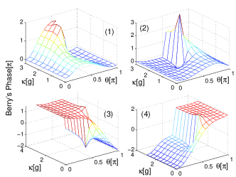
Figure 1: The Berry phase $\gamma_{n,ab}^{0}$ for the bipartite system in a no-jump trajectory as a function of the decoherence rate $\kappa$ and the azimuthal angle $\theta$. (1)-(4) in the figure correspond to different instantaneous eigenstates $|\Psi_{j}\rangle$, $j=1,2,3,4$.

The numerical results for the Berry phase with no-jump were presented in figure 1, where we plot $\gamma_{n,ab}^{0}$ $(n=1,2,3,4)$ as a function of the spontaneous rate $\kappa$ and the azimuthal $\theta$. In contrast with the case of $\kappa=0$ yi04 , there are jumps at $\theta=\pi/2$ with $\kappa>\kappa_{0}$ depending on the path the system follows. The jumps appearing in figure 1 may be understood as follows. The evolution of the state along the no-jump trajectory represented by one of equation (17) can be mapped on the Bloch sphere with spontaneous decay rate $\sim\kappa$. The evolution is then a smooth spiral converging to the lower state, thus the geometric phase increases due to the spontaneous decay when the initial state falls onto the upper semi-sphere; while the phase decrease when it initially is in the lower semi-sphere. Therefore, the geometric phase has a jump at the crossover point $\theta=\pi/2$. This was schematically shown in figure 2.

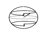
Figure 2: A schematic illustration for the effect of spontaneous decay. The solid angle increases due to the decay when the state is on the upper sphere, while it decreases for that on the lower sphere.

In the case where only one quantum jump (described by operator $\sigma_{a}^{-}$) occurs at any time $t_{1}$, the geometric phase shift due to the jump is given by

$$\gamma_{n,ab}^{jump}=\mbox{arg}\{a_{n}C_{n}^{*}+b_{n}D_{n}^{*}\},\mbox{\ \ }(n=1,2,3,4),$$ (20)

selected numerical results for $\gamma_{n,ab}^{jump}$ were illustrated in figure 3. The quantum jump occurring at a time of $\phi=\pi$ was assumed for this plot. Clearly, singularity appears at $\theta=\pi/2$, where the subsystem $a$ experiences a crossover from the upper half of the Bloch sphere to the lower one.

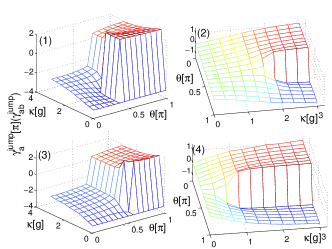
Figure 3: Geometric phase acquired by the bipartite system (or subsystem $a$) in a single quantum jump among the adiabatic path $|\Psi_{j}\rangle$. The quantum jump was assumed to occur at the time when $\phi=\pi$.

In conclusion, we have investigated the geometric phase in open bipartite systems. This study is of relevance to the geometric quantum computing, where geometric phase may be used to perform quantum information processing. To our best knowledge, this issue remains unaddressed by the trajectory approach, in particular for coupled open systems. The results show that there is a singularity in the dependance of the geometric phase on the azimuthal angle with a specific $\kappa>\kappa_{0}$, where $\kappa_{0}$ depends on the inter-subsystem coupling constant $g$. The phase shift due to the quantum jump was also calculated, it has shown that the phase shift depends strongly on the direction to which the spin-$\frac{1}{2}$ particle points. The jump occurs at $\theta=\pi/2$ can be interpreted in picture of the Bloch sphere, in which the decaying of the subsystem $a$ results in a smooth spiral converging to the ground state, so when the state falls in the upper semi-sphere, the decay increases the geometric phase, but it lowers the geometric phase when the state on another semi-sphere, this leads to the jump in the phase at $\theta=\pi/2$. And it is interesting to note that there is no jump when the decay rate $\kappa<\kappa_{0}$, the critical value of the decay, this is due to that the system finishes a cyclic evolution before the system decay.

This work was supported by NCET of M.O.E, and NSF of China Project No. 10305002.

References

- (1) M. V. Berry, Proc. R. Soc. London A 392, 45(1984).
- (2) Geometric phase in physics, Edited by A. Shapere and F. Wilczek ( World Scientific, Singapore, 1989).
- (3) P. Zanardi and M. Rasetti, Phys. Lett. A 264, 94 (1999).
- (4) J. A. Jones, V. Vedral, A. Ekert, and G. Castagnoli, Nature (London) 403, 869 (1999).
- (5) A. Ekert, M. Ericsson, P. Hayden, H. Inamori, J.A. Jones, D.K.L. Oi, and V. Vedral, J. Mod. Opt. 47, 2051 (2000).
- (6) G.Falci, R. Fazio, G.M. Palma, J. Siewert, and V. Vedral, Nature (London) 407, 355 (2000).
- (7) A. Uhlmann, Rep. Math. Phys. 24, 229 (1986).
- (8) E. Sjöqvist, A.K. Pati, A. Ekert, J.S. Anandan, M. Ericsson, D.K.L. Oi, and V. Vedral, Phys. Rev. Lett. 85, 2845 (2000).
- (9) J. C. Garrison and E. M. Wright, Phys. Lett. A 128, 177(1988).
- (10) D. Ellinas, S. M. Barnett, and M. A. Dupertuis, Phys. Rev. A 39, 3228(1989).
- (11) D. Gamliel and J. H. Freed, Phys. Rev. A 39, 3238(1989).
- (12) F. Gaitan, Phys. Rev. A 58, 1665(1998).
- (13) K. M. Fonseca Romero, A. C. Aguira Pinto, and M. T. Thomaz, Physica A 307, 142(2002).
- (14) A. Nazir, T. P. Spiller, W. J. Munro, Phys. Rev. A 65, 042303(2002).
- (15) A. C. Aguira Pinto and M. T. Thomaz, J. Phys. A: Math. Gen. 36, 7461(2003).
- (16) A. Carollo, I. Fuentes-Guridi, M. Franca Santos and V. Vedral, Phys. Rev. Lett. 90,160402(2003); ibid 92, 020402(2004).
- (17) R. S. Whitney, and Y. Gefen, Phys. Rev. Lett. 90, 190402(2003); R. S. Whitney, Y. Makhlin, A. Shnirman, and Y. Gefen, e-print:cond-mat/0405267.
- (18) I. Kamleitner, J. D. Cresser, and B. C. Sanders, Phys. Rev. A 70, 044103(2004).
- (19) K. P. Marzlin, S. Ghose, and B. C. Sanders, Phys. Rev. Lett. 93, 260402 (2004).
- (20) E. Sjöqvist, Phys. Rev. A 70, 052109(2004).
- (21) X. X. Yi, L. C. Wang, and W. Wang, Phys. Rev. A 71, 044101 (2005).
- (22) G. Dattoli, R. Mignani, and A. Torre, J. Phys. A 23, 5395(1990).
- (23) G. Lindblad, Commun. Math. Phys. 48, 119 (1976).
- (24) X.X. Yi, L.C. Wang, and T.Y. Zheng, Phys. Rev. Lett. 92, 150406 (2004); X. X. Yi, and E. Sjöqvist, Phys. Rev. A 70, 042104 (2004).
- (25) M. Ericsson, E. Sjöqvist, J. Brannlund, D. K. L. Oi, and A. K. Pati, Phys. Rev. A 67, 020101(2003).