Experimenter’s Freedom in Bell’s Theorem and Quantum Cryptography

Abstract

Bell’s theorem states that no local realistic explanation of quantum mechanical predictions is possible, in which the experimenter has a freedom to choose between different measurement settings. Within a local realistic picture the violation of Bell’s inequalities can only be understood if this freedom is denied. We determine the minimal degree to which the experimenter’s freedom has to be abandoned, if one wants to keep such a picture and be in agreement with the experiment. Furthermore, the freedom in choosing experimental arrangements may be considered as a resource, since its lacking can be used by an eavesdropper to harm the security of quantum communication. We analyze the security of quantum key distribution as a function of the (partial) knowledge the eavesdropper has about the future choices of measurement settings which are made by the authorized parties (e.g. on the basis of some quasi-random generator). We show that the equivalence between the violation of Bell’s inequality and the efficient extraction of a secure key — which exists for the case of complete freedom (no setting knowledge) — is lost unless one adapts the bound of the inequality according to this lack of freedom.

I Introduction

Can the experimenter’s free-will be experimentally tested? It seems unreasonable to expect that this question can be answered unconditionally. The philosophical debate on whether or not our choices are ultimately up to ourselves or are just a predetermined illusion has lasted for centuries without reaching a final conclusion. Here we pursue our profession as physicists reminding ourselves of Einstein’s words that ”It is the theory which decides what we can observe”. Thus, roughly speaking, one could say that it is the theory that decides whether or not the experimenter’s free-will can be tested. Here we consider the experimenter’s freedom of choosing between different possible measurement settings and argue that, within a local realistic theory, it can experimentally be tested. Following Gill et al. gill this freedom will be defined as the independence of the experimenter’s choice of measurement settings from the local realistic mechanism that determines the actual measurement results.

The theorem of John Bell bell states the impossibility of a local realistic explanation of quantum mechanics in which the experimenter has a freedom to choose between different experimental arrangements. This is demonstrated by the experimental confirmation of the violation of Bell’s inequalities in agreement with quantum mechanical predictions. The philosophical implications of Bell’s theorem are startling: either one must abandon the experimenter’s freedom, or the view that external reality exists prior to and independent of observations (realism), or dramatically revise our concepts of space and time (locality). Needless to say, either of the choices requires radical revision of the ruling philosophical view of most of the scientists and is in sharp contrast to our every-day experience.

If one chooses to keep a local realistic picture and to deny the experimenter’s freedom, then one must accept a world in which the measurement settings that are generated by the experimenter’s choice (or by tossing a coin, or — to put it in a grotesque way — by the parity of the number of cars passing the laboratory within $n$ seconds, where $n$ is given by the fourth decimal of the cube of the actual temperature in degrees Fahrenheit) are determined in advance and correlated with the actual outcome of the measurement. Bell himself comments such theories with the words bell1 : ”A theory may appear in which such conspiracies inevitably occur, and these conspiracies may then seem more digestible than the non-localities of other theories. When that theory is announced I will not refuse to listen, either on methodological or other grounds. But I will not myself try to make such a theory.”

In this paper we show that the experimentally observed degree of violation of Bell’s inequalities sets a minimal degree to which the free choice has to be abandoned if one insists on a local realistic explanation. Thus, not every local realistic theory denying free choice is in agreement with observations. Finally, extending the idea of Hwang hwang , we argue that the experimenter’s freedom can be considered as a resource in quantum communication as its lacking can be used by an eavesdropper to harm its security. We analyze the security in quantum key distribution as a function of the knowledge the eavesdropper has about the choice of measurement settings which is made by the authorized parties in the protocol.

II Bell’s Inequalities with Reduced Experimenter’s Freedom

Realism supposes that the measurement results are determined by ”hidden variables” which exist prior to and independent of observation. Locality supposes that the results obtained at one location are independent of any measurements or actions performed at space-like separated regions. Finally, ”freedom of choice” assumes that the experimenter’s choice of the measurement setting is independent of the local realistic mechanism which determines the measurement results. In what follows we pursue the approach of Gill et al. gill in formulating these concepts in a mathematically rigorous way.

Consider two spatially separated partners, Alice and Bob, performing space-like separated experiments on particles which are pairwise emitted by some source. Let $X$ and $Y$ denote the actual measurement outcomes obtained, and $k$ and $l$ the actual measurement settings chosen by Alice and Bob, respectively. The outcomes $X$ and $Y$ can take values $+1$ or $-1$, and the settings $k$ and $l$ values $1$ or $2$. The probability to observe the two outcomes to be equal, $X\!=\!Y$, under the chosen $k$ (Alice) and $l$ (Bob) is denoted by $P(X\!=\!Y|kl)$.

Local realism assumes the existence of a quadruple of variables $\{X_{1},X_{2},Y_{1},Y_{2}\}$, each taking values $+1$ or $-1$, which represents the potential measurement outcomes in a thought experiment, under any of the possible measurement settings. This quadruple exists independently of whether any or which experiment is actually performed on either side. Because of locality the variables on Alice’s side do not depend on the choice of setting on Bob’s side, and vice versa. Thus, local realism requires $X\in\{X_{1},X_{2}\}$ and $Y\in\{Y_{1},Y_{2}\}.$

The freedom assumption expresses the independence between the choice $k,l$ of the measurement settings and the local realistic mechanism which finally selects the actual outcomes ${X,Y}$ from the potential ones ${X_{1},X_{2},Y_{1},Y_{2}}$. Gill et al. gill put this formally in the requirement that $\{k,l\}$ are statistically independent of $\{X_{1},X_{2},Y_{1},Y_{2}\}$. This means that in many thought repetitions of the experiment the probabilities with which the quadruple $\{X_{1},X_{2},Y_{1},Y_{2}\}$ takes on any of its $2^{4}$ possible values remain the same within each subensemble defined by the four possible combinations of $k$ and $l$. In particular, one has $P(X_{k}\!=\!Y_{l})\!=\!P(X\!=\!Y|kl)$, where $P(X_{k}\!=\!Y_{l})$ is the (mathematical) probability for having $X_{k}=Y_{l}$.

What if the experimenter’s freedom is just an illusion? Imagine that the choices of experimental settings and experimental results are both consequences of some common local realistic mechanism. In such a case the two probabilities $P(X_{k}\!=\!Y_{l})$ and $P(X\!=\!Y|kl)$ may differ from each other and we use their difference

$$\Delta_{kl}\equiv P(X\!=\!Y|kl)-P(X_{k}\!=\!Y_{l})$$ (1)

to measure the lack of freedom. This measure can acquire values from $-1$ to $1$, and the freedom case corresponds to all $\Delta_{kl}=0$. It is important to note that while the probabilities $P(X\!=\!Y|kl)$ can directly be measured, the $P(X_{k}\!=\!Y_{l})$ are only mathematical entities of the local realistic theory without a direct operational meaning. Nevertheless, they satisfy a set-theoretical constraint which is mathematically equivalent to the Clauser–Horne–Shimony–Holt (CHSH) inequality chsh . The product of local realistic results $X_{2}Y_{2}$ is always equal to the multiplication of $(X_{1}Y_{1})(X_{1}Y_{2})(X_{2}Y_{1})$, because the square of a dichotomic variable, with values $+1$ or $-1$, is equal to $+1$. This implies that the following expression can attain only one of two values gill :

$$\openone\{X_{1}=Y_{1}\}+\openone\{X_{1}=Y_{2}\}$$

$$+\openone\{X_{2}=Y_{1}\}-\openone\{X_{2}=Y_{2}\}=0\text{ or }2\,,$$ (2)

where $\openone\{X_{k}=Y_{l}\}$ is the indicator of the event $X_{k}=Y_{l}$, i.e., it is equal to $1$ if it happens and $0$ if it does not happen. The expectation value of the indicator variable is the probability for the event to happen, $P(X_{k}\!=\!Y_{l})$. Finally the expectation value of the left-hand side cannot be greater than the maximum value of the averaged expression:

$$S_{\text{CHSH}} \equiv P(X_{1}\!=\!Y_{1})+P(X_{1}\!=\!Y_{2})$$

$$\quad+P(X_{2}\!=\!Y_{1})-P(X_{2}\!=\!Y_{2})\leq 2\,.$$ (3)

The equivalence to the CHSH inequality is evident as soon as one recalls that the correlation function of dichotomic variables equals $E_{kl}=2P(X_{k}\!=\!Y_{l})-1$. The above inequality, in turn, implies a new bound on the set of probabilities that can experimentally be measured:

$$S_{\Delta} \equiv P(X\!=\!Y|11)+P(X\!=\!Y|12)$$ (4)

$$\quad+P(X\!=\!Y|21)-P(X\!=\!Y|22)\leq 2+\Delta_{\text{CHSH}},$$

where $\Delta_{\text{CHSH}}\equiv\Delta_{11}+\Delta_{12}+\Delta_{21}-\Delta_{22}$. Note that on the basis of measured probabilities (relative frequencies) one cannot make statements about the individual measures $\Delta_{kl}$ but rather on their combination as given in $\Delta_{\text{CHSH}}$. In particular, it is possible that $\Delta_{\text{CHSH}}\!=\!0$, although all the individual $\Delta_{kl}\!\neq\!0$, and it may also be negative. However, only the case of positive $\Delta_{\text{CHSH}}$ — implying at least one individual $\Delta_{kl}$ to be unequal to zero — makes the freedom assumption within a local realistic model experimentally testable, as the bound on the right-hand side of (4) is increased. As well one could study the lower bounds of $S_{\text{CHSH}}$ and $S_{\Delta}$.

To give an example of the lack of freedom model, imagine a local realistic mechanism in which the source ”knows” in advance the settings “to be chosen” by Alice and Bob. The source can ”arbitrarily” manipulate the value of $S_{\Delta}$ in this case. Even the algebraic (logical) bound of $S_{\Delta}=3$ can be reached: whenever Alice and Bob both measure the second setting, the source sends (local realistic) correlated pairs such that the measurement results anticoincide, i.e. $P(X\!=\!Y|22)=0$, and in all other measurements it produces pairs for which the results coincide, i.e. $P(X\!=\!Y|11)=P(X\!=\!Y|12)=P(X\!=\!Y|21)=1$, and thus $S_{\Delta}=3$. For this local realistic model (without freedom) inequality (4) is satisfied, but only because of the adapted bound $2+\Delta_{\text{CHSH}}=3$. Now imagine another experiment, in which the observers (freely) choose their settings independently from the local realistic source. Then $P(X\!=\!Y|kl)=P(X_{k}\!=\!Y_{l})$, i.e. $\Delta_{\text{CHSH}}=0$, and inequality (4) is fulfilled with the bound of 2, as it becomes the CHSH inequality (3).

The value of $\Delta_{\text{CHSH}}$ for which the inequality is still satisfied, defines the minimal extent to which the experimenter’s freedom has to be abandoned such that a local realistic explanation of the experiment is still possible. Denote the left-hand side of inequality (4) as the CHSH expression. The maximal possible quantum value, $S_{\text{QM}}=1+\sqrt{2}$, of this expression can be observed for the maximally entangled state, for example, the singlet state $|\psi^{-}\rangle=(|0\rangle|1\rangle-|1\rangle|0\rangle)/\sqrt{2}$, where $|0\rangle$ and $|1\rangle$ are two orthogonal quantum states, and for an appropriate choice of possible settings $\{k,l\}$. This quantum value requires an abandonment of the experimentalist’s freedom to the extent of at least $\Delta_{\text{CHSH}}=\sqrt{2}-1\approx 0.414$.

Since, based on the experiment, we can only make statements about $\Delta_{\text{CHSH}}$, a large number of local realistic theories are possible that deny the experimenter’s freedom and are in agreement with quantum mechanical predictions and experiments. In order to be able to make further statements about these theories we need to impose some structure on them. In what follows we restrict ourselves to the case where the degree to which the freedom is abandoned — that is the absolute value of the measure $\Delta_{kl}$ — is independent of the actual experiment performed, i.e. $|\Delta_{kl}|\!=\!\Delta$ is the same for all $k,l$. Roughly speaking, the level of conspiracy is assumed to be the same for all experimental situations. Choosing $\Delta_{11}\!=\!\Delta_{12}\!=\!\Delta_{21}\!=\!-\Delta_{22}\!\equiv\!\Delta$ one obtains $\Delta=\frac{1}{4}(\sqrt{2}-1)\approx 0.104$ for the minimal degree required to explain the quantum value of the CHSH expression by a local realistic model. If all the $\Delta_{kl}$ are positive (i.e. if $P(X\!=\!Y|kl)>P(X_{k}\!=\!Y_{l})$ for all $k,l$), one finds the even higher value $\Delta=\frac{1}{2}(\sqrt{2}-1)\approx 0.207$.

It is known that with an increasing number of parties, $N$, the discrepancy between the results of Bell tests and local realistic predictions that respect the experimenter’s freedom increases rapidly (exponentially) with $N$ mermin . We now determine how the degree of the lack of freedom needs to scale with $N$ in a local realistic theory that agrees with these tests.

Consider $N$ space-like separated parties who can each choose between two possible measurement settings. Let $X^{(j)}\!\in\!\{1,-1\}$ denote the actual measurement result obtained and $k_{j}\!\in\!\{1,2\}$ the actual measurement setting chosen by party $j$. The probability to observe correlation, i.e. the probability that the product of local results is equal to $1$ if settings $k_{1},...,k_{N}$ are chosen, is denoted by $P(\prod_{j=1}^{N}\!X^{(j)}\!=\!1|k_{1}...k_{N})$. Local realism assumes the existence of $2\,N$ numbers $\{X_{1}^{(1)},X_{2}^{(1)},...,X_{1}^{(N)},X_{2}^{(N)}\}$, each taking values $+1$ or $-1$ and representing the potential measurement outcomes of $N$ parties under any possible combination of their measurement settings. The (mathematical) probability that the product of the potential outcomes is equal to $1$ is denoted by $P(\prod_{j=1}^{N}\!X_{k_{j}}^{(j)}\!=\!1)$. Note again that this probability cannot be measured experimentally.

We apply the approach used above to the present case of $N$ parties. We introduce the difference

$$\Delta_{k_{1}...k_{N}}\equiv P(\textstyle\prod_{j=1}^{N}\!X^{(j)}\!=\!1|k_{1}...k_{N})-P(\textstyle\prod_{j=1}^{N}\!X_{k_{j}}^{(j)}\!=\!1)$$ (5)

to measure the lack of freedom of $N$ experimenters. The probabilities $P(\prod_{j=1}^{N}\!X_{k_{j}}^{(j)}\!=\!1)$ satisfy a set-theoretical constraint that is mathematically equivalent to the Mermin inequality mermin (the particular form used here is from zukowski ):

$$M\equiv\!\sum_{k_{1},...,k_{N}=1}^{2}\!s(k_{1},...,k_{N})\,P(\textstyle\prod_{j=1}^{N}\!X_{k_{j}}^{(j)}\!=\!1)\leq B(N)\,,$$ (6)

where $s(k_{1},...,k_{N})\!=\!\sin\!\left[(k_{1}+...+k_{N})\frac{\pi}{2}\right]$ are coefficients taking values $0$, $+1$ or $-1$. The inequality is bounded by $B(N)\!=\!\frac{1}{2}\!\left[2^{\lfloor N/2\rfloor}\!+\!2^{N/2}\sin(\frac{N\pi}{4})\right]$, where $\lfloor x\rfloor$ is the greatest integer less or equal to $x$. Using inequality (6) and definition (5), one obtains a new inequality:

$$M_{\Delta} \equiv\!\sum_{k_{1},...,k_{N}=1}^{2}\!s(k_{1},...,k_{N})\,P(\textstyle\prod_{j=1}^{N}\!X^{(j)}\!=\!1|k_{1}...k_{N})$$

$$\leq B(N)+\Delta_{\text{Merm}},$$ (7)

where $\Delta_{\text{Merm}}\!=\!\sum_{k_{1},...,k_{N}=1}^{2}s(k_{1},...,k_{N})\,\Delta_{k_{1}...k_{N}}$. Importantly, the probabilities entering this inequality are measurable.

In a Bell experiment involving the maximally entangled $N$-party (GHZ) state one observes $M_{\text{QM}}=\frac{1}{2}\left[2^{N-1}+2^{N/2}\sin(\frac{N\pi}{4})\right]$ for the maximal possible value of the left-hand side of inequality (7). This implies $2^{N-2}-2^{\lfloor(N-2)/2\rfloor}$ for the minimal value of $\Delta_{\text{Merm}}=M_{\text{QM}}-B(N)$ that still allows a local realistic explanation of the experiment. Suppose again that the degree of the lack of freedom is independent of the measurement setting. With an adequate choice of signs one has $\Delta_{k_{1}...k_{N}}\!=\!\Delta_{N}$ for $k$’s for which $s(k_{1},...,k_{N})\!=\!1$ and $\Delta_{k_{1}...k_{N}}\!=\!-\Delta_{N}$ for $k$’s for which $s(k_{1},...,k_{N})\!=\!-1$. This results in $\Delta_{\text{Merm}}\!=\!2^{N-1}\Delta_{N}$. Finally, one obtains that the degree to which the experimenter’s freedom has to be abandoned in order to have an agreement between local realism and Bell’s experiments with $N$ parties saturates exponentially fast with $N$ as $\Delta_{N}=\frac{1}{2}-\frac{1}{2^{\lfloor(N+1)/2\rfloor}}$. In the limit of infinitely many partners $\Delta_{N}$ reaches the value of $\frac{1}{2}$. It is remarkable that if the sign of all $\Delta_{k_{1}...k_{N}}$ is chosen positive, there will be no way to obtain agreement between local realism and the experimental results, since $\Delta_{N}$ would have to leave the range from $-1$ to $+1$ in the limit of large $N$. The other argument which invalidates all $\Delta_{k_{1}...k_{N}}$ to be positive involves only four parties. In this case in the expression defined in (7) the number of probabilities with a positive sign is equal to the number of probabilities with a negative sign. Thus, if all $\Delta_{k_{1}...k_{N}}$ are positive and have the same value they cancel each other, i.e. $\Delta_{\text{Merm}}=0$, and no explanation of the violation of the bound $B(N\!=\!4)$ is possible.

In this section we showed that quantum correlations for $N$ partners can be explained within local realism only if both the number of measurement settings in which the experimenter’s freedom is abandoned (all $2^{N-1}$ combinations of local settings entering the Mermin inequality) increases exponentially and the degree of this abandonment saturates exponentially fast with $N$. Furthermore, from the viewpoint of local realism that denies freedom, there is no obvious reason why the quantum bound of the CHSH inequality is $1+\sqrt{2}$ and not, for example, the maximal possible logical bound of 3. In our opinion these objections clearly show that the local realistic program goes squarely against every effort for simple and sensible explanations of our observations. In particular, in order to explain the violation of Bell’s inequality within local realism, one has to introduce purely theoretical and experimentally not accessible entities such as the (mathematical) probabilities $P(X_{k}\!=\!Y_{l})$. This is against the spirit of Ockham’s razor principle.

III Quantum Key Distribution with Reduced Experimenter’s Freedom

The violation of Bell’s inequality by legitimate parties was found to be a necessary and sufficient condition for their efficient extraction of a quantum secret key gisin ; acin , showing an appealing connection between secure key distribution and the violation of local realism.

Apart from its fundamental meaning, the freedom to choose between different measurement settings can be regarded as an important resource in quantum secret key distribution. In particular, as recently shown by Hwang hwang , an eavesdropper can both simulate the violation of Bell’s inequality and successfully eavesdrop, if the freedom in choosing the settings by legitimate partners is abandoned. Effectively, one can assume that each measurement device chooses its settings according to a pseudo-random sequence that is installed in the device beforehand. Such a model of lack of freedom allows the eavesdropper to know the algorithm generating the pseudo-random numbers, at least to some extent, and correspondingly predict the future measurement settings of the legitimate parties.

In what follows we will consider an Ekert-like protocol ekert — a combination of the BBM92 protocol bennet (which is an application of the BB84 protocol bb84 to entangled states) and a CHSH test — and analyze both the violation of Bell’s inequality and the security of the key distribution as a function of the amount of knowledge that the eavesdropper Eve (E) has about the settings chosen by the legitimate parties Alice (A) and Bob (B). We have chosen this combination of BBM92 and CHSH — henceforth denoted as the BBM–CHSH protocol — because it allows to test the relationship between Bell’s theorem and secure quantum key distribution in a single protocol. (In contrast to the original Ekert protocol with non-orthogonal key establishing settings, there is a security proof for the BBM92 attached to the error rate.)

Consider a source that emits pairs of spin-$\frac{1}{2}$ particles in the singlet state $|\psi^{-}\rangle=(|z+\rangle|z-\rangle-|z-\rangle|z+\rangle)/\sqrt{2}$, where $|z+\rangle$ and $|z-\rangle$ denote spin-up and spin-down along the $z$-direction, respectively. The legitimate parties measure the incoming particles in the $x,y$-plane. Alice can choose between two orthogonal settings, characterized by the azimuthal angles $\alpha_{1}\equiv 0$ and $\alpha_{2}\equiv\frac{\pi}{2}$, whereas Bob has 4 possible measurement directions, namely $\beta_{1}\equiv\alpha_{1}\equiv 0$, $\beta_{2}\equiv\alpha_{2}\equiv\frac{\pi}{2}$, $\beta_{3}\equiv\frac{\pi}{4}$, and $\beta_{4}\equiv\frac{3\pi}{4}$ (note that the $\beta_{j}$ are not numbered in ascending order). Therefore, depending on their choice of settings, they sometimes measure correlations for determining the violation of the CHSH inequality, namely with the 4 settings $(\alpha_{1},\beta_{3})$, $(\alpha_{1},\beta_{4})$, $(\alpha_{2},\beta_{3})$, and $(\alpha_{2},\beta_{4})$, or they can establish a key, since their outcomes are perfectly anti-correlated for measurements along $(\alpha_{1},\beta_{1})$ and $(\alpha_{2},\beta_{2})$. If they choose $(\alpha_{1},\beta_{2})$ or $(\alpha_{2},\beta_{1})$, i.e. orthogonal directions, they discard their results. A schematic of the measurement directions is shown in figure 1.

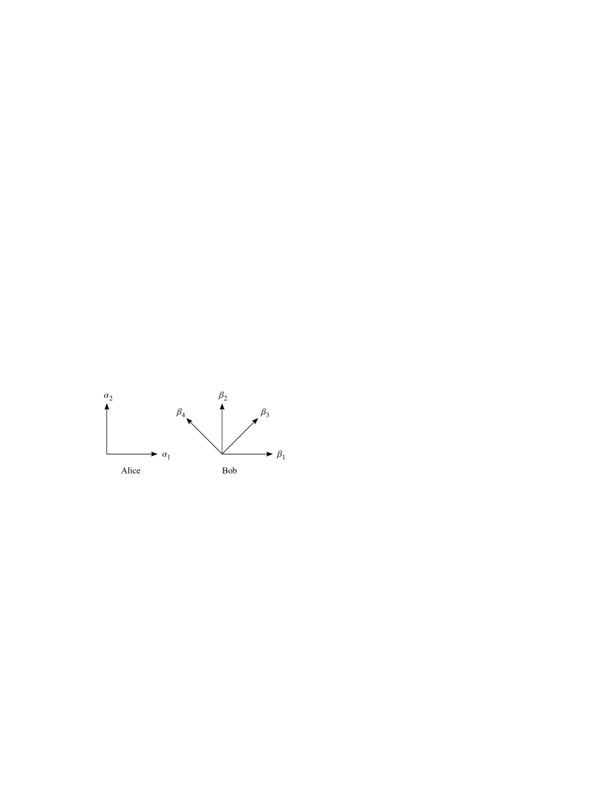
Figure 1: Settings in the BBM–CHSH protocol. Alice chooses between two orthogonal measurement directions $\alpha_{1}$ and $\alpha_{2}$, whereas Bob has four different possibilities, namely the same directions as Alice, i.e., $\beta_{1}$ and $\beta_{2}$, as well as two directions rotated by $\frac{\pi}{4}$, i.e. $\beta_{3}$ and $\beta_{4}$.

Let $P(X\!=\!-Y|ij)$ denote the probability that Alice and Bob obtain anti-correlated results if they measure along $\alpha_{i}$ and $\beta_{j}$, respectively, where $i=1,2$ and $j=1,2,3,4$. Within the freedom assumption the (measured) CHSH expression has the form

$$S \equiv P(X\!=\!-Y|13)+P(X\!=\!-Y|23)$$

$$\quad+P(X\!=\!-Y|24)-P(X\!=\!-Y|14)\leq 2\,.$$ (8)

For the (maximally entangled) singlet state it is equal to $1+\sqrt{2}$. The classical bound is 2, whereas the logical bound is equal to 3.

Let us now assume that an eavesdropper, Eve, has some knowledge about the choice of settings of Alice and Bob, for instance by having some insight into their random number generators. We model this knowledge in the following way: In each run, i.e., for each singlet pair, Eve knows that the combination of local settings $(\alpha_{i},\beta_{j})$ will happen with probability $q_{ij}$. For simplicity we assume that one out of the 8 joint settings will happen with (high) probability $Q\geq\tfrac{1}{8}$, whereas all the others 7 have equal (low) probability $\frac{1-Q}{7}$ to be manifested. The number $Q$ shall be the same for all runs; the setting which it indicates to be most probable of course changes from run to run. The case $Q=1$ corresponds to perfect knowledge of the eavesdropper and to the complete lack of free will of Alice and Bob, whereas $Q=\tfrac{1}{8}$ means that Eve has no knowledge at all.

Now we impose the following attack algorithm: If Eve believes one of the CHSH settings to be most likely, she sends the corresponding optimal product state. In general, if $q_{ij}=Q$, which means that the setting $(\alpha_{i},\beta_{j})$ is most probable from Eve’s viewpoint, she intercepts and sends either $\left|\alpha_{i}\right\rangle_{\text{A}}\left|\beta_{j}+\pi\right\rangle_{\text{B}}$ or $\left|\alpha_{i}+\pi\right\rangle_{\text{A}}\left|\beta_{j}\right\rangle_{\text{B}}$ (by tossing a fair coin, such that the local results of Alice and Bob are always totally random). Only in the special case $q_{14}=Q$, Eve sends $\left|\alpha_{1}\right\rangle_{\text{A}}\left|\beta_{4}\right\rangle_{\text{B}}$ or $\left|\alpha_{1}+\pi\right\rangle_{\text{A}}\left|\beta_{4}+\pi\right\rangle_{\text{B}}$. This is the CHSH setting where the probability of anti-correlation should be minimized, since $P(X\!=\!-Y|14)$ appears with a minus sign in the CHSH inequality. Therefore, she attacks the CHSH measurements in order to achieve a maximal violation ($S=3$) and the key establishing measurements to find the key (or rather produce it herself).

To further motivate why we have chosen this attack algorithm, we note that (i) it is canonical in the way that Eve attacks all events in the same way, namely with the appropriate product state. (ii) The attack is already good enough to show that the connection between violation of local realism and secure key distribution is lost in the case where the eavesdropper has partial knowledge about the settings. (iii) Eve sends a product state for each pair that is generated by the source; hence, Alice and Bob are faced with measurement results that can be described by local realism but nevertheless can violate the CHSH inequality (8) due to restricted freedom.

According to Eve’s setting knowledge and the attack strategy, one can compute the value for the CHSH expression as measured by Alice and Bob. In the subensemble of cases where, e.g., Alice measures along $\alpha_{1}$ and Bob along $\beta_{3}$, Eve sends with probability $Q$ the product states resulting in anti-correlations $P(X\!=\!-Y|13)=1$. In the rest of the cases she sends 7 possible ”wrong guesses” which each happen with probability $\frac{1-Q}{7}$ and for each of them the probability for anti-correlations takes values between $\frac{1}{2}$ and $\cos^{2}\!\frac{\pi}{8}\approx 0.854$, depending on the specific wrong attack. The measured probability $P(X\!=\!-Y|13)$ is the expectation value of all 8 sets of anti-correlated results weighted with their probabilities to happen. Analogously, the probabilities for anti-correlation in the other subensembles are calculated and we find

$$P(X\! =\!-Y|13)=Q+\tfrac{1-Q}{7}\left(\tfrac{5}{2}+2\,\cos^{2}\!\tfrac{\pi}{8}\right)\!,$$ (9)

$$P(X\! =\!-Y|23)=P(X\!=\!-Y|13)\,,$$ (10)

$$P(X\! =\!-Y|24)=Q+\tfrac{1-Q}{7}\left(\tfrac{5}{2}+\cos^{2}\!\tfrac{\pi}{8}+\sin^{2}\!\tfrac{\pi}{8}\right)\!,$$ (11)

$$P(X\! =\!-Y|14)=\tfrac{1-Q}{7}\left(\tfrac{5}{2}+\cos^{2}\!\tfrac{\pi}{8}+\sin^{2}\!\tfrac{\pi}{8}\right)\!.$$ (12)

The CHSH expression finally results in

$$S=3\,Q+\tfrac{1-Q}{7}\left(5+4\,\cos^{2}\!\tfrac{\pi}{8}\right)\approx 1.2+1.8\,Q\,.$$ (13)

Thus, the logical bound $S_{\text{log}}\equiv 3$ is reached in the limit $Q\rightarrow 1$. The classical bound of $S_{\text{cl}}\equiv 2$ is beaten for all $Q>Q_{\text{cl}}\approx 0.44$ and the quantum mechanics (Cirel’son) bound $S_{\text{qm}}\equiv 1+\sqrt{2}\approx 2.41$ is beaten for setting knowledge $Q>Q_{\text{qm}}\approx 0.67$. If $Q$ is larger than $Q_{\text{qm}}$, Eve should reduce the strength of her attack, e.g. by mixing some noise into her product states, for otherwise even the quantum bound would be broken. The CHSH expression (13) and the bounds are shown in figure 2a.

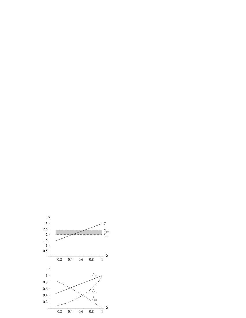
Figure 2: (a) The (measured) CHSH expression $S$ as a function of Eve’s setting knowledge $Q$ (solid line). The CHSH inequality (8) with classical bound $S_{\text{cl}}=2$ (dotted line) is violated for every setting knowledge $Q>Q_{\text{cl}}\approx 0.44$. The quantum bound $S_{\text{qm}}=1+\sqrt{2}$ is also indicated. (b) The mutual information between Alice and Bob $I_{\text{AB}}$ (dashed line) and the actual mutual information between Bob and Eve $I_{\text{BE}}$ (solid line), which is always smaller than (or equal to) the Alice–Eve mutual information. For every setting knowledge $Q$ one has $I_{\text{BE}}\geq I_{\text{AB}}$ and thus Alice and Bob can never extract a secret key. An optimal attack without setting knowledge leads to $\tilde{I}_{\text{BE}}$ (dotted line). Only for $Q\leq Q_{0}\approx 0.63$ the BBM–CHSH protocol is secure, because Alice and Bob find $I_{\text{AB}}\leq\tilde{I}_{\text{BE}}$ and they will not use their key.

We can make the direct connection with section II, where now Eve plays the role of ”conspiratorial” local realistic nature. Accordingly, we can introduce the difference between the measured probabilities $P(X\!=\!-Y|ij)$ and their mathematical (set constraint fulfilling) counterparts $P(X_{i}\!=\!-Y_{j})$ to which the experimenter has no access. The latter are given by the first if one substitutes the value $Q=\tfrac{1}{8}$ as this corresponds to the case where Eve has no setting knowledge and Alice and Bob are receiving a classical mixture of equally weighted product states for each run: $P(X_{i}\!=\!-Y_{j})=P(X\!=\!-Y|ij)|_{Q=1/8}$. The difference

$$\Delta_{ij}\equiv P(X\!=\!-Y|ij)-P(X_{i}\!=\!-Y_{j})$$ (14)

measures the lack of freedom. The set constraint fulfilling CHSH expression is

$$S_{\text{CHSH}} \equiv P(X_{1}\!=\!-Y_{3})+P(X_{2}\!=\!-Y_{3})$$

$$\quad+P(X_{2}\!=\!-Y_{4})-P(X_{1}\!=\!-Y_{4})\leq 2\,,$$ (15)

and therefore

$$S\leq 2+\Delta_{\text{CHSH}}\,,$$ (16)

where $\Delta_{\text{CHSH}}\equiv\Delta_{13}+\Delta_{23}+\Delta_{24}-\Delta_{14}$. Inequality (16) is fulfilled if and only if (15) is fulfilled and this is the case because the (mathematical) probabilities $P(X_{i}\!=\!-Y_{j})$ correspond to a mixture of product states and therefore obey local realism.

When is Eve’s knowledge about the settings also sufficient to find out the key which is established by Alice and Bob? To answer this question, we have to compute mutual informations between the parties. The mutual information between Alice and Bob is determined by the bit error rate gisin which they can compute in the subensembles where they measured along $\alpha_{1}\!=\!\beta_{1}\!=\!0$ or $\alpha_{2}\!=\!\beta_{2}\!=\!\frac{\pi}{2}$. Let us consider the first; the error rate in the second is the same for symmetry reasons. The bit error rate $D$ is given by the sum of 8 terms corresponding to the 8 settings that were potentially possible from Eve’s point of view. Each term is the probability with which Eve believed this event would happen — $Q$ for the event $(\alpha_{1},\beta_{1})$ itself and $\frac{1-Q}{7}$ for all the others (the wrong guesses), corresponding to our definition of the setting knowledge — multiplied with the probability that the attack $(\alpha_{i},\beta_{j})$ leads to a correlation (error) rather than an anti-correlation as for the original singlet state. This ”destruction probability” is $0$ for the ”correct” event $(\alpha_{1},\beta_{1})$, it is $\sin^{2}\!\frac{\pi}{8}$ for both $(\alpha_{1},\beta_{3})$ and $(\alpha_{1},\beta_{4})$, and $\frac{1}{2}$ for all the others (where an orthogonal state was sent to Alice or Bob). Finally, we find the bit error rate

$$D=\tfrac{1-Q}{7}\left(\tfrac{5}{2}+2\,\sin^{2}\!\tfrac{\pi}{8}\right)\approx 0.4\,(1-Q)\,.$$ (17)

The mutual information between Alice and Bob is

$$I_{\text{AB}}\equiv 1-H(D)\,,$$ (18)

with $H(p)\equiv-p\lg p-(1-p)\lg(1-p)$ the Shannon entropy, where lg denotes the logarithm with base 2.

The maximal mutual information between Alice (or Bob for symmetry reasons) and Eve from Alice’s and Bob’s viewpoint, which can be attained by an optimal attack of Eve for a given error rate $D$ and under the condition that Eve has no setting knowledge, is given by gisin

$$\tilde{I}_{\text{AE}}=\tilde{I}_{\text{BE}}=1-H(\tfrac{1}{2}\!+\!\sqrt{D-D^{2}})\,.$$ (19)

The actual mutual information between Alice and Eve, $I_{\text{AE}}$, can be computed from the conditional entropy $H_{\text{A}|\text{E}}$ by $I_{\text{AE}}=H_{\text{A}}-H_{\text{A}|\text{E}}$, where Alice’s Shannon information is $H_{\text{A}}=1$, since the outcomes of Alice are always locally random for all possible attacks. As all chosen settings are publicly revealed after the measurements, Eve can compute $H_{\text{A}|\text{E}}$ in the subensemble of the key establishing measurement $(\alpha_{1},\beta_{1})$. (If Alice and Bob measure along $(\alpha_{2},\beta_{2})$, the result does not change.) The calculation itself is straightforward, once one realizes that $H_{\text{A}|\text{e}}=0$ for all 4 events e in which Eve (justly) believed that Alice would choose $\alpha_{1}$, as Eve knows her result in this case. If Eve made the (wrong) guess $\alpha_{2}$ then $H_{\text{A}|\text{e}}=1$ for these 4 possible events, for Alice measures in the orthogonal direction $\alpha_{1}$. Thus, $H_{\text{A}|\text{E}}=4\,\frac{1-Q}{7}$ and

$$I_{\text{AE}}=1-4\,\tfrac{1-Q}{7}=\tfrac{3}{7}+\tfrac{4}{7}\,Q\,.$$ (20)

Analogously, one can find the actual mutual information between Bob and Eve:

$$I_{\text{BE}}=1-\tfrac{1-Q}{7}\left(2+4\,H(\cos^{2}\!\tfrac{\pi}{8})\right)\approx 0.37+0.63\,Q\,,$$ (21)

which is always smaller than (or equal to) $I_{\text{AE}}$. Secret-key agreement between Alice and Bob using only error correction and privacy amplification is possible if and only if the Alice-Bob mutual information is greater than the minimum of the Alice–Eve and Bob–Eve mutual information, that is, if and only if $I_{\text{AB}}>\min(I_{\text{AE}},I_{\text{BE}})$ csiszar . We have

$$I_{\text{AB}}\leq I_{\text{BE}}$$ (22)

for all $Q$ and equality only holds for $Q=1$. Alice and Bob can never extract a secret key, since the condition $I_{\text{AB}}>I_{\text{BE}}$ is never fulfilled (figure 2b).

The well-known critical error rate $D_{0}=\tfrac{1}{2}\,(1-\tfrac{1}{\sqrt{2}})\approx 0.15$ corresponds, according to (17), to a setting knowledge $Q_{0}\approx 0.63$. For this knowledge $I_{\text{AB}}=\tilde{I}_{\text{BE}}$. If $Q>Q_{0}$, the BBM–CHSH protocol is insecure, since $I_{\text{AB}}\leq I_{\text{BE}}$ and Alice and Bob find both their error rate to be sufficiently small (below $D_{0}$) and the CHSH inequality (8) to be violated, which makes them think they are safe. For $Q\leq Q_{0}$ Eve’s setting knowledge is ”insufficient” and the protocol becomes secure: Alice and Bob cannot extract a secret key because still $I_{\text{AB}}<I_{\text{BE}}$, but they find $I_{\text{AB}}\leq\tilde{I}_{\text{BE}}$ and know that there might be an eavesdropper and thus they will not use the key. For $0.44\approx Q_{\text{cl}}<Q\leq Q_{0}\approx 0.63$ they will find the CHSH inequality (8) to be violated ($S>2$) and nonetheless they cannot extract a secret key ($I_{\text{AB}}\leq\tilde{I}_{\text{BE}}$, $D\geq D_{0}$). Therefore, we deduce that the equivalence between the violation of Bell’s inequality (with complete freedom) and the secure key distribution (without freedom) is lost. (However, the new bound in inequality (16) is never broken and, in fact, a secret key can never be extracted.)

If Alice and Bob knew $Q$, which means they knew to which extent their freedom is restricted, and if they calculated the maximal $\Delta_{\text{CHSH}}$ under the constraint of an insecure key, $I_{\text{AB}}\leq\min(I_{\text{AE}},I_{\text{BE}})$, for all possible attacks, then a violation of the CHSH inequality with the new bound $2+\Delta_{\text{CHSH}}$ would be equivalent to the possibility of efficient secret key extraction (unless the new bound is larger than $S_{\text{qm}}=1+\sqrt{2}$). A violation of this new bound is equivalent to statement that the classical bound 2 is violated in the case of total freedom and for this situation there exists a complete equivalence between the CHSH inequality violation and the security of the BBM protocol gisin ; acin .

IV Conclusions

The violation of Bell’s inequalities is an experimental fact. Within a local realistic program this fact can only be explained if the experimenter’s freedom in choosing between different measurement settings is denied (modulo known loopholes, considered by most scientists to be of technical nature). For a local realist our results show that both the number of settings in which the freedom is abandoned grows exponentially and the degree of this abandonment saturates exponentially fast with the number of parties. For the present authors, however, these results are rather an indication of the absurdity of the program itself. Nevertheless, they give rise to new security criteria for quantum cryptography in situations in which the measurement settings chosen by the authorized parties are partially revealed by an eavesdropper. This contradicts the standard assumption in cryptography in which the laboratories of the authorized parties are safe and no relevant information is allowed to leak out from them. If this assumption is not fulfilled, we showed that the violation of the standard CHSH inequality is not equivalent to a secure key distribution anymore. Nevertheless, it is possible to define a new (higher) bound whose violation indeed guarantees the security of the key. Therefore, one can keep the security while, to some extent, relaxing the assumption that no information is revealed to an eavesdropper, as long as the amount of this information is known.

References

- (1) R. D. Gill, G. Weihs, A. Zeilinger, and M. Żukowski, Proc. Nat. Acad. Sci. USA, 9, 14632 (2002); R. D. Gill, G. Weihs, A. Zeilinger, and M. Żukowski, Europhys. Lett. 61, 282 (2003).
- (2) J. S. Bell, Physics (Long Island City, N.Y.), 1, 195 (1964).
- (3) J. S. Bell, Free Variables and Local Causality, Dialectica 39, 103-106 (1985).
- (4) W.-Y. Hwang, Phys. Rev. A 71, 052329 (2005).
- (5) J. F. Clauser, M. Horne, A. Shimony, and R. Holt, Phys. Rev. Lett. 23, 880 (1969).
- (6) N. D. Mermin, Phys. Rev. Lett. 65, 1838 (1990).
- (7) M. Żukowski and Č. Brukner, Phys. Rev. Lett. 88, 210401 (2002).
- (8) N. Gisin, G. Ribordy, W. Tittel, and H. Zbinden, Rev. Mod. Phys. 74, 145 (2002).
- (9) V. Scarani and N. Gisin, Phys. Rev. Lett. 87, 117901 (2001); A. Acin, N. Gisin, L. Masanes, and V. Scarani, Int. J. Quant. Inf. 2, 23 (2004).
- (10) A. K. Ekert, Phys. Rev. Lett. 67, 661 (1991).
- (11) C. H. Bennett, G. Brassard, and N. D. Mermin, Phys. Rev. Lett. 68, 557 (1992).
- (12) C. H. Bennet and G. Brassard, Proceedings of the IEEE Int. Conf. on Computers, Systems and Signal Processing, Bangalore (1984).
- (13) I. Csiszár and J. Körner, IEEE Trans. Inf. Theory IT-24, 339 (1978).