Overdamping by weakly coupled environments

Abstract

A quantum system weakly interacting with a fast environment usually undergoes a relaxation with complex frequencies whose imaginary parts are damping rates quadratic in the coupling to the environment, in accord with Fermi’s “Golden Rule”. We show for various models (spin damped by harmonic-oscillator or random-matrix baths, quantum diffusion, quantum Brownian motion) that upon increasing the coupling up to a critical value still small enough to allow for weak-coupling Markovian master equations, a new relaxation regime can occur. In that regime, complex frequencies lose their real parts such that the process becomes overdamped. Our results call into question the standard belief that overdamping is exclusively a strong coupling feature.

I Introduction

The dynamics of an isolated and finite quantum system consists of a reversible superposition of oscillations with (real) Bohr frequencies $\omega_{S}$. In order to understand the irreversible processes occurring in finite quantum systems, such as relaxation to equilibrium or decoherence, one needs to take into account the interaction between the system and its environment. The weak-interaction limit together with the Markovian approximation already allow a good understanding of such irreversible processes and has some universal features. The generator of the evolution of the (reduced) density matrix of the system obtained by second-order perturbation theory (often called the Redfieldian) is not an anti-Hermitian generator any more. Its eigenvalues $\Gamma+{{\rm i}}\Omega$ acquire a real part $\Gamma$ describing irreversible decay to equilibrium. The imaginary parts of the eigenvalues are shifted Bohr frequencies $\Omega=\omega_{S}-\delta\omega$. The two shifts $\Gamma$ and $\delta\omega$, normally increase (quadratically) as the strength of the coupling grows.

We here propose to show that Markovian perturbative master equations such as the Redfield equation Red ; Kampen ; HaaSpring ; KuboB2 ; GaspRed ; BreuPet ; Esposito allow for more than just describing the well known normal damping just mentioned. When the coupling strength is increased, it can happen at a critical value that a shifted frequency $\Omega$ vanishes and for yet stronger coupling goes imaginary. The pertinent eigenvalues $\Gamma-|\Omega|$ are real and, interestingly, decrease with growing coupling. The resulting relaxation is non-oscillatory, i.e. overdamped. The principle purpose of this paper is to show that contrary to common belief the transition to overdamping is still compatible with perturbative treatment. In brief, overdamping can be a weak-coupling effect.

All models to be studied here have Hamiltonians like

$$\hat{H} = \hat{H}_{S}+\hat{H}_{B}+\hat{S}\hat{B}\,,$$ (1)

where $\hat{H}_{S}$ and $\hat{H}_{B}$ respectively generate the free motion of the system and the environment (bath) while the interaction involves respective coupling agents $\hat{S}$ and $\hat{B}$.

It may be well to emphasize that the so-called rotating-wave approximation Gardiner ; BreuPet , extremely useful as it may be for very weak damping, in particular in quantum optics, is definitely not allowable for strong damping and overdamping. Indeed, the rotating-wave approximation is based on the assumption that the Bohr frequencies of the system are very large compared to the system damping rate such that all “anti-resonant” terms can be time averaged out when writing the master equation in the interaction picture. But overdamping occurs precisely when the Bohr frequencies of the system become of the order of or smaller then the system damping rate. In a recent study of low-quality resonators Hacken , the rotating-wave approximation was shown to be still affordable for overlapping resonances. But the Hamiltonians to be employed in the present paper must retain the “anti-resonant” terms that the rotating-wave approximation would suppress.

A word on physical contexts where overdamping shows up is in order. One such is diffusion, a topic to be dealt with below (Section III). Another one is temporal fluctuations in critical phenomena, described by time dependent Ginzburg-Landau equations without inertial terms HHM ; Ref. Bausch describes a derivation of such a Ginzburg-Landau equation from an underlying unitary evolution of a “larger” system.

The plan of the paper is as follows: In section II, we solve the Redfield master equation for a two-level system interacting with a general environment. When the environment is made of harmonic oscillators (spin-boson model), we show in subsection II.2 that the transition from normal damping to overdamping occurs at a critical value of the coupling which can be made arbitrarily small and therefore accessible to perturbation theory. For environment operators $\hat{H}_{B}$ and $\hat{B}$ modeled by random matrices from the so-called Gaussian orthogonal ensemble (spin-GORM model), we show in subsection II.3 that weak-coupling overdamping is compatible with the exact dynamics computed numerically. In section III, we show that the transition from a non-diffusive to a diffusive regime, recently identified for a particle traveling in a spatially extended system while interacting with an environment, corresponds in fact to a transition from normal damping to overdamping; that transition will turn out amenable to perturbative analysis. Finally, in section IV we study the transition from normal damping to overdamping for a central harmonic oscillator interacting with a large collection of harmonic oscillators (quantum Brownian motion). We show that overdamping again allows for perturbative treatment, by comparison with the exact results known for this model. Conclusion are drawn in section V.

II Damped spin

II.1 Hamiltonian and Markovian master equation

Any two-level system has the Pauli matrices $\hat{\sigma}_{x},\hat{\sigma}_{y},\hat{\sigma}_{z}$ (together with unity) as a complete set of observables. If such a “spin” interacts with a general environment we may choose the Hamiltonian as

$$\hat{H}=\frac{\hbar\omega_{0}}{2}\hat{\sigma}_{z}+\hat{H}_{B}+\hat{\sigma}_{x}\hat{B}\,.$$ (2)

Inasmuch as the interaction $\hat{\sigma}_{x}\hat{B}$ does not commute with the Hamiltonians for the uncoupled spin and bath, it allows for transitions between the unperturbed energy levels. Denoting the means of the spin observables by

$$x(t)=\textrm{Tr}\hat{\rho}(t)\hat{\sigma}_{x},\;\;y(t)=\textrm{Tr}\hat{\rho}(t)\hat{\sigma}_{y},\;\;z(t)=\textrm{Tr}\hat{\rho}(t)\hat{\sigma}_{y}$$ (3)

we write the Redfield equation as GaspRed ; Esposito

$$\dot{z}(t) = 2\Gamma\,(z(\infty)-z(t))$$ (4)

$$\dot{x}(t) = -\omega_{0}y(t)$$

$$\dot{y}(t) = \frac{(\Omega^{2}+\Gamma^{2})}{\omega_{0}}x(t)-2\Gamma y(t)\,,$$

with the time dependent damping rate $\Gamma(t)$ and frequency $\Omega(t)$ and the stationary inversion $z(\infty)$

$$\Gamma(t) = \frac{2}{\hbar^{2}}\int_{0}^{t}d\tau\cos(\omega_{0}\tau)\;C(\tau)$$ (5)

$$\Omega(t)^{2}+\Gamma(t)^{2} = \omega_{0}^{2}+\frac{4}{\hbar^{2}}\omega_{0}\int_{0}^{t}d\tau\sin(\omega_{0}\tau)\;C(\tau)$$

$$\Gamma(t)\;z(\infty) = \frac{2}{\hbar^{2}}\int_{0}^{t}d\tau\sin(\omega_{0}\tau)\;D(\tau)\,.$$

Properties of the bath are represented by the functions $C(t)$ and $D(t)$, respectively the real and imaginary parts of the equilibrium autocorrelation function $\alpha(t)=\langle B(t)B(0)\rangle$ of the bath coupling agent $B$ (For definition and properties see appendix A).

The Markovian approximation consists in taking the upper bounds of the time integrals in (5) to infinity, such that the damping constant and frequency become time independent, $\Gamma(\infty)\equiv\Gamma,\Omega(\infty)\equiv\Omega\,$. That approximation is legitimate when the spin dynamics characterized by the rates $\omega_{0},\Omega,\Gamma$ is much slower than the decay of the bath correlation function $\alpha(t)$ and requires that we restrict the further discussion to times much larger than the bath correlation time. We may then rewrite (5) as

$$\Gamma = \frac{\pi}{\hbar^{2}}(\tilde{\alpha}(\omega_{0})+\tilde{\alpha}(-\omega_{0}))$$ (6)

$$\Omega^{2}+\Gamma^{2} = \omega_{0}^{2}+\frac{4}{\hbar^{2}}\omega_{0}^{2}\int d\omega{\cal P}\frac{\tilde{\alpha}(\omega)}{\omega_{0}^{2}-\omega^{2}}$$

$$z(\infty) = \frac{\tilde{\alpha}(-\omega_{0})-\tilde{\alpha}(\omega_{0})}{\tilde{\alpha}(-\omega_{0})+\tilde{\alpha}(\omega_{0})}\,,$$

with $\tilde{\alpha}(\omega)$ the Fourier transform of $\alpha(t)$. The solutions of equations (4) in the Markovian limit read

$$z(t) = z(\infty)+(z(0)-z(\infty))\,{\rm e}^{-2\Gamma t}$$ (7)

$$x(t) = \frac{x(0)\Gamma-y(0)\omega_{0}}{\Omega}\sin\left(\Omega t\right){\rm e}^{-\Gamma t}$$

$$+x(0)\cos\left(\Omega t\right){\rm e}^{-\Gamma t}$$

$$y(t) = \frac{x(0)((\Omega^{2}+\Gamma^{2})/\omega_{0})-y(0)\Gamma}{\Omega}\sin\left(\Omega t\right){\rm e}^{-\Gamma t}$$

$$+y(0)\cos\left(\Omega t\right){\rm e}^{-\Gamma t}.$$

The reduced density matrix $\rho=\frac{1}{2}+x\hat{\sigma}_{x}+y\hat{\sigma}_{y}+z\hat{\sigma}_{z}$ can thus be written as a superposition of four modes,

$$\hat{\rho}(t)=\sum_{\xi=1}^{4}c_{\xi}(0)\,\hat{\rho}^{\xi}\,{\rm e}^{s_{\xi}t}\,.$$ (8)

For normal damping, $s_{1}=0$, $s_{2}=-2\Gamma$, $s_{3}=-\Gamma+{{\rm i}}\Omega$ and $s_{4}=-\Gamma-{{\rm i}}\Omega$. Overdamping occurs when

$$\Omega^{2}<0\,,$$ (9)

and then the rates of (8) are given by $s_{1}=0$, $s_{2}=-2\Gamma$, $s_{3}=-\Gamma+|\Omega|$ and $s_{4}=-\Gamma-|\Omega|$.

II.2 The spin-boson model

Taking the bath as a collection of harmonic oscillators Leggett ; GaspRed we have for its free Hamiltonian and coupling agent

$$\hat{H}_{B} = \frac{1}{2}\sum_{n=1}^{N}(\hat{P}^{2}_{n}+\omega_{n}^{2}\hat{Q}^{2}_{n})\,,\quad B=\sum_{n=1}^{N}\epsilon_{n}\hat{Q}_{n}.$$ (10)

We assume a quasi-continuum of bath frequencies $\omega_{n}$, employ a spectral function $\gamma(\omega)=\sum_{n}\epsilon_{n}^{2}\delta(\omega_{n}-\omega)$, and adopt Ullersma’s choice [see Ullersma and Appendix A],

$$\gamma(\omega)=\frac{2}{\pi}\frac{\kappa\alpha^{2}\omega^{2}}{\alpha^{2}+\omega^{2}}\,,$$ (11)

where $\alpha$ is the decay rate of the autocorrelator of the bath coupling agent and $\kappa$ an overall coupling strength. Thus equipped we can evaluate the rates in (5). In the limits of high temperature, i.e. $\beta\hbar\omega_{0}\equiv\hbar\omega_{0}/k_{B}T\ll 1$, we get

$$\Gamma \stackrel{{\scriptstyle\beta\to 0}}{{=}} 2\frac{\kappa\alpha^{2}}{\beta\hbar^{2}(\alpha^{2}+\omega_{0}^{2})}\,\stackrel{{\scriptstyle\frac{\omega_{0}}{\alpha}\to 0}}{{=}}\,\frac{2\kappa}{\beta\hbar^{2}}$$ (12)

$$\Omega^{2}+\Gamma^{2} \stackrel{{\scriptstyle\beta\to 0}}{{=}} \omega_{0}^{2}+4\frac{\kappa\alpha\omega_{0}^{2}}{\beta\hbar^{2}(\alpha^{2}+\omega_{0}^{2})}\stackrel{{\scriptstyle\frac{\omega_{0}}{\alpha}\to 0}}{{=}}\omega_{0}^{2}$$ (13)

$$\Gamma\;z(\infty) = -\frac{\kappa\alpha^{2}\omega_{0}}{\hbar(\alpha^{2}+\omega_{0}^{2})}\stackrel{{\scriptstyle\frac{\omega_{0}}{\alpha}\to 0}}{{=}}-\frac{\kappa\omega_{0}}{\hbar}\,;$$ (14)

here the limit $\omega_{0}/\alpha\to 0$ has been taken to remain consistent with the Markovian approximation; note that in the present section $\kappa$ has the dimension of an action, such that $\Gamma$ is a rate.

The critical value of $\kappa$ at which overdamping occurs is now found with the help of Eq. (9) by subtracting Eq.(12) to the power two to Eq. (13). We find

$$\kappa_{c} \stackrel{{\scriptstyle\beta\to 0}}{{=}} \frac{\hbar^{2}\beta\omega_{0}}{2}$$ (15)

If $\kappa>\kappa_{c}$, and if $\kappa_{c}$ is small enough to be treated by perturbation theory we have a selfconsistent theory of overdamping. Clearly, high temperatures are favorable for that theory to apply since the pertinent $\kappa_{c}$ is suppressed by the factor $\beta\hbar\omega_{0}\ll 1$.

One might fear that our way of obtaining $\kappa_{c}$ is not completely consistent if solely restricted to second-order perturbation theory because $\Gamma^{2}$ is of order $\kappa^{2}$ while $\Omega^{2}+\Gamma^{2}$ is of order $\kappa$ and does not include the $\kappa^{2}$ corrections. That fear would be eased by the following argument. If we were to add ${\cal O}(\kappa^{2})$ corrections to the right-hand sides of Eqs. (12,13), the results (15) for the critical coupling would be generalized to series in powers of the leading terms displayed in (15). (In fact, Jang et al. Ref.Silbey found $\Omega^{2}+\Gamma^{2}=\omega_{0}^{2}(1+4\kappa^{2}/\hbar^{2})$; by recalculating $\kappa_{c}$, we again find Eq. (15) if $\beta\hbar\omega_{0}\ll 1$.)

Another look at the high-temperature rates reveals an interesting feature of overdamping. We have from (8)

$$s_{1} = 0$$ (16)

$$s_{2} = -\frac{4\kappa}{\hbar^{2}\beta}$$

$$s_{3} = -\frac{2\kappa}{\hbar^{2}\beta}+\frac{2\kappa}{\hbar^{2}\beta}\sqrt{1-\left(\frac{\kappa_{c}}{\kappa}\right)^{2}}$$

$$s_{4} = -\frac{2\kappa}{\hbar^{2}\beta}-\frac{2\kappa}{\hbar^{2}\beta}\sqrt{1-\left(\frac{\kappa_{c}}{\kappa}\right)^{2}}\,.$$

Most remarkably, the slowest relaxation rate of the spin, $|{\rm Re}[s_{3}]|$, decreases when the coupling to the environment increases. For strong overdamping, $\kappa_{c}/\kappa\ll 1$, we even have

$$s_{3}=-\frac{\beta\omega_{0}^{2}}{4\kappa}+{\cal O}(\frac{\hbar^{2}\beta^{3}\omega_{0}^{4}}{\kappa^{3}})\;.$$ (17)

This is in contrast to the normal-damping case, accessible from the above by replacing $\sqrt{-1}\to+{{\rm i}}$, where the two slowest rates $|{\rm Re}[s_{2}]|$ and $|{\rm Re}[s_{3}]|$ increase as the coupling becomes stronger.

II.3 The spin-GORM model

We retain the overall Hamiltonian (2) but modify the environment so as to let the free-bath Hamiltonian $\hat{H}_{B}$ and the coupling agent $\hat{B}$ be represented by random matrices from the Gaussian orthogonal ensemble (GOE). The resulting spin-GORM model was studied in Refs. Esposito ; EspoGasp2 . We use the results of that work; in particular, we adopt a unit of time that makes the Hamiltonian dimensionless and the bath correlation time of order $\hbar$ (see Eq.(19) below). Specifically, we write

$$\hat{H}_{B}=\frac{\hat{X}}{\sqrt{8N}}\,,\quad\hat{B}=\eta\frac{\hat{X}^{{}^{\prime}}}{\sqrt{8N}}\,;$$ (18)

here $\hat{X}$ and $\hat{X}^{{}^{\prime}}$ are random $\frac{N}{2}\times\frac{N}{2}$ GOE matrices with mean zero. Their non-diagonal (resp. diagonal) elements have standard deviation $\sigma_{ND}=1$ (resp. $\sigma_{D}=\sqrt{2}$). The parameter $\eta$ serves as a coupling strength.

To study this model it is convenient to assume that the environment is initially in a microcanonical distribution with the (dimensionless) energy $\epsilon$. The autocorrelator of the bath coupling agent then reads

$$\alpha(\epsilon,t)\stackrel{{\scriptstyle N\to\infty}}{{=}}\eta^{2}\frac{J_{1}(t/(2\hbar))}{4t/\hbar}\,{\rm e}^{{{\rm i}}\epsilon t/\hbar}$$ (19)

and has the Fourier transform

$$\tilde{\alpha}(\epsilon,\omega)\stackrel{{\scriptstyle N\to\infty}}{{=}}\frac{\eta^{2}\hbar}{2\pi}\sqrt{\frac{1}{4}-(\epsilon+\hbar\omega)^{2}}\,.$$ (20)

It may be well to note that we here meet Wigner’s semi-circle law for the mean level density of the GOE.

The general rates of the Markovian Redfield equation given in Eq. (6) can be evaluated and read

$$\Gamma(\epsilon)=\frac{\eta^{2}}{2\hbar}\!\left[\!\sqrt{\frac{1}{4}-(\epsilon-\hbar\omega_{0})^{2}}+\sqrt{\frac{1}{4}-(\epsilon+\hbar\omega_{0})^{2}}\right]$$ (21)

and

$$\Omega(\epsilon)^{2}+\Gamma(\epsilon)^{2} = \omega_{0}^{2}+\eta^{2}\omega_{0}^{2}$$

$$-\frac{\eta^{2}}{\hbar}\omega_{0}\frac{\sqrt{(\epsilon+\hbar\omega_{0})^{2}-\frac{1}{4}}}{\pi}\arctan\left(\frac{(\epsilon+\hbar\omega_{0})+\frac{1}{2}}{\sqrt{(\epsilon+\hbar\omega_{0})^{2}-\frac{1}{4}}}\right)$$

$$-\frac{\eta^{2}}{\hbar}\omega_{0}\frac{\sqrt{(\epsilon+\hbar\omega_{0})^{2}-\frac{1}{4}}}{\pi}\arctan\left(\frac{(\epsilon+\hbar\omega_{0})-\frac{1}{2}}{\sqrt{(\epsilon+\hbar\omega_{0})^{2}-\frac{1}{4}}}\right)$$

$$+\frac{\eta^{2}}{\hbar}\omega_{0}\frac{\sqrt{(\epsilon-\hbar\omega_{0})^{2}-\frac{1}{4}}}{\pi}\arctan\left(\frac{(\epsilon-\hbar\omega_{0})+\frac{1}{2}}{\sqrt{(\epsilon-\hbar\omega_{0})^{2}-\frac{1}{4}}}\right)$$

$$+\frac{\eta^{2}}{\hbar}\omega_{0}\frac{\sqrt{(\epsilon-\hbar\omega_{0})^{2}-\frac{1}{4}}}{\pi}\arctan\left(\frac{(\epsilon-\hbar\omega_{0})-\frac{1}{2}}{\sqrt{(\epsilon-\hbar\omega_{0})^{2}-\frac{1}{4}}}\right).$$

If $\Omega^{2}<0$, we have overdamping. To discuss that case, we momentarily set $\Omega^{2}=A-B$ where $A=\Omega^{2}+\Gamma^{2}$ and is given by (21) and $B=\Gamma^{2}$ by (II.3). When $\eta$ is large we could have overdamping because $B>A$, but then perturbation theory may fail and our approach lose selfconsistency. However, since all terms in $A$ (but none in $B$) carry explicit factors $\omega_{0}$ or $\omega_{0}^{2}$, and since the other quantities containing $\omega_{0}$ (i.e. $\sqrt{.}$ and $\arctan(.)$) are bounded away from zero in the limit $\omega_{0}\to 0$, it is always possible to choose $\omega_{0}$ sufficiently small such that $A<B$ for small $\eta$. This is illustrated in Fig. 1.

Figure 1: $\eta=0.2$, $\epsilon=0$ and $\hbar=1$. This figure shows that the condition for overdamping can be satisfied at weak coupling if $\omega_{0}$ is sufficiently small. This is still true for any generic choice of $\epsilon$.

Figure 2: $\omega_{0}=0.01$, $\epsilon=0$ and $\hbar=1$. The upper figure shows that for a fixed and small value of $\omega_{0}$ their exist a critical and small value of the coupling $\eta_{c}\approx 0.14$ above which overdamping occurs. The lower figure illustrates the qualitative change of the coupling dependence of the slowest relaxation rates when going from the normal damping regime to the overdamped regime.

The dependence of the smallest rates on the coupling strength is similar as in the spin-boson model. The rates $|{\rm Re}[s_{3}]|$ and $|{\rm Re}[s_{4}]|$ [see Eqs. (8)], grow with the coupling constant $\eta$ in the normal-damping regime, have a cusp at the transition, and then decay into the regime of overdamping, as illustrated in Fig. 2.

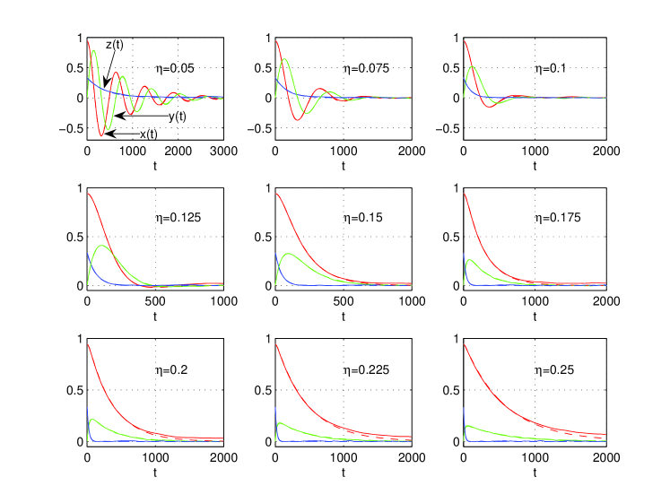
Figure 3: (Color online) Transition from normal damping to overdamping in the spin-GORM model. The full lines represent the exact dynamics of the three spin observable $x(t),y(t),z(t)$ obtained numerically by diagonalizing the full Hamiltonian and the dashed lines represent the dynamics predicted by the Redfield equation (second order perturbation theory). The two results give curves which are so close to each other that the dashed lines are almost invisible. The situation depicted here is the same as in Fig. 2 where $\eta$ varies and $\omega_{0}=0.01$, $\epsilon=0$ and $\hbar=1$. As predicted by Redfield theory, the transition occurs at $\eta_{c}\approx 0.14$. The initial condition is $x(0)=\sqrt{8}/3,y(0)=0,z(0)=1/3$. For the exact dynamics we have taken $N=3000$ and a width of the initial energy shell $\delta\epsilon=0.025$.

We have numerically solved the exact dynamics in order to verify that the perturbative equation predicts the correct dynamics for normal damping as well as for overdamping. The agreement is excellent as illustrated in Fig. 3. We can conclude that the spin-GORM model allows for overdamping at weak coupling.

III Diffusion model

We now consider a particle moving on one dimensional closed loop while interacting with an environment. The pertinent dynamics has been studied recently in Refs. Esposito ; EspoGaspdiff1 ; EspoGaspdiff2 by using the Redfield equation. A transition from nondiffusive to diffusive relaxation has been identified. We shall here use the results of this study to show that the transition mentioned in fact is one from normal damping to overdamping.

The Hamiltonian of the loop constituting the subsystem is represented by an $N\times N$ matrix

$$\hat{H}_{S}=\left(\begin{array}[]{ccccccc}E_{0}&-A&0&0&\ldots&0&-A\\ -A&E_{0}&-A&0&\ldots&0&0\\ 0&-A&E_{0}&-A&&0&0\\ \vdots&&\ddots&\ddots&\ddots&&\vdots\\ 0&0&&-A&E_{0}&-A&0\\ 0&0&\ldots&0&-A&E_{0}&-A\\ -A&0&\ldots&0&0&-A&E_{0}\\ \end{array}\right)_{N\times N}$$ (30)

taken in the site basis ${|l\rangle}$, where $l=0,1,\ldots,N-1$ labels the $N$ sites on the loop. The diagonal elements of $\hat{H}_{S}$ are the on-site energies of the particle while the offdiagonal elements generate hopping to neighboring sites.

A weak interaction with an environment is described by the Redfield master equation. The correlation time of the environment is assumed much shorter than all characteristic time scales of the loop and therefore the correlation function of the environment can be modeled by

$$\alpha_{ll^{\prime}}(\tau)=2\;Q\;\delta(\tau)\;\delta_{ll^{\prime}}\,.$$ (31)

By using the Bloch theorem, the Redfield generator (containing $N^{4}$ elements) can be simplified in $N$ independent sectors (with $N^{2}$ elements), corresponding each to a given value of the Bloch number $q$. For our finite loop periodicity yields $q=n2\pi/N$, where $n=1,2,\ldots,N$. By diagonalizing a given sector we get $N$ eigenvalues depending on $q$. The complete spectrum of the Redfield generator then consists of the $N^{2}$ eigenvalues obtained by varying $q$.

As already mentioned, two relaxation regimes have been identified in this model. In the nondiffusive regime all eigenvalues are complex with real parts of similar magnitude, proportional to the coupling constant $Q$,

$${\rm Re}[s]\approx-\frac{2Q}{\hbar^{2}}+{\cal O}(\frac{1}{N})\,.$$ (32)

However, in a given sector (therefore at a given $q$) when the coupling term is increased beyond the value $Q=2\hbar A\sin\frac{q}{2}$, one of the $N$ eigenvalues separates from the other $N-1$ ones. This eigenvalue is always real and is called the diffusive one. The diffusive branch is made of the diffusive eigenvalues of the different sectors. These eigenvalues have a smaller magnitude than the real parts of the nondiffusive eigenvalues. They therefore control the long time relaxation of the subsystem. The diffusive eigenvalues are given by

$$s=-\frac{2Q}{\hbar^{2}}+\frac{2Q}{\hbar^{2}}\sqrt{1-\left(\frac{2\hbar A}{Q}\sin\frac{q}{2}\right)^{2}}.$$ (33)

Lets define $Q_{c}\equiv 2\hbar A\sin\frac{\pi}{N}\approx 2\pi\hbar A/N$. For $Q<Q_{c}$ no diffusive eigenvalues are present in the spectrum and the relaxation regime is nondiffusive [see Eq. (32)]. As soon as $Q>Q_{c}$, at least two diffusive eigenvalues exist in the spectrum and the relaxation regime is called the diffusive regime. The two smallest diffusive eigenvalues controlling the long time scale relaxation are

$$s=-\frac{4\pi^{2}A^{2}}{QN^{2}}\,.$$ (34)

Notice that the perturbative approach is consistent, because $Q_{c}$ can be made as small as desired by choosing $A/N$ small.

It is already clear at this point that the nondiffusive (resp. diffusive) regime implies normal damping (resp. overdamping). Indeed, as for normal damping (resp. overdamping), the smallest relaxation rates increase (resp. decrease) with growing coupling in the nondiffusive (resp. diffusing) regime. Furthermore, as in the normal damping (resp. overdamping) regime, the small Redfield eigenvalues are complex (resp. real) in the nondiffusive (resp. diffusing) regime. We can make that association even clearer if we assume the environment made of harmonic oscillators which we model by using Ullersma’s spectral density [see appendix (A)]. In this case, we find that at high temperature, the zero-frequency limit of the Fourier transform of the environment correlation function is given by

$$\lim_{\omega\to 0}\tilde{\alpha}(\omega)=\lim_{\omega\to 0}\frac{J(\omega)}{\omega}=\frac{\kappa}{\pi\beta}\,.$$ (35)

Since our instantaneous-decay assumption (31) implies

$$\tilde{\alpha}(0)=\frac{Q}{\pi}$$ (36)

we conclude

$$Q=\frac{\kappa}{\beta}$$ (37)

and thus find the diffusive-branch eigenvalues

$$s = -\frac{2\kappa}{\hbar^{2}\beta}+\frac{2\kappa}{\hbar^{2}\beta}\sqrt{1-(4\hbar A\sin(\frac{q}{2})\frac{\beta}{2\kappa})^{2}}$$

$$= -\frac{\beta A^{2}}{\kappa}q^{2}+{\cal O}(\frac{\hbar^{2}\beta^{3}A^{4}}{\kappa^{3}}q^{4}).$$

The similarity between these diffusive eigenvalues and the smallest eigenvalue of the spin-boson model in the overdamping regime [$s_{3}$ in Eq. (16)] is obvious, as is similarity between the real part of the small nondiffusive eigenvalues [(32) with (37)] and the real parts of the small eigenvalues of the spin-boson model in the normal damping regime [$s_{3}$ and $s_{4}$ in (16)].

IV Quantum Brownian Motion (QBM)

IV.1 Hamiltonian

In this section we study overdamping in an exactly solvable model of Brownian motion. The model is made of a central harmonic oscillator interacting with an environment which itself is a collection of harmonic oscillators (see, e.g. Ullersma ; Haake ; Zurek ; BreuPet ; these references will lead the reader to earlier work). The exact solution proves extremely valuable for our endeavor since it will be seen to yield, in the Markovian limit, precicely the same condition for overdamping as the perturbative treatment.

We write the total QBM Hamiltonian as Rem1

$$\hat{H}=\frac{1}{2}(\hat{P}^{2}+\omega_{0}^{2}\hat{Q}^{2})+\frac{1}{2}\!\sum_{n=1}^{N}\!\!\Big{(}\!\hat{P}^{2}_{n}+\omega_{n}^{2}(\hat{Q}_{n}-\frac{\epsilon_{n}}{\omega_{n}^{2}}\hat{Q})^{2}\!\Big{)}$$ (39)

and thus have the system and bath parts

$$\hat{H}_{S} = \frac{1}{2}\Big{(}\hat{P}^{2}+\big{(}\omega_{0}^{2}+\sum_{n=1}^{N}\frac{\epsilon_{n}^{2}}{\omega_{n}^{2}}\big{)}\hat{Q}^{2}\Big{)}\,,$$ (40)

$$\hat{H}_{B} = \frac{1}{2}\sum_{n=1}^{N}\Big{(}\hat{P}^{2}_{n}+\omega_{n}^{2}\hat{Q}^{2}_{n}\Big{)}\,.$$ (41)

The coupling agents of system and bath read

$$\hat{S}=\hat{Q}_{0},\ \ ;\ \ \hat{B}=-\sum_{n=1}^{N}\epsilon_{n}\hat{Q}_{n}\,.$$ (42)

The QBM Hamiltonian (39) is a sum of squares and thus manifestly positive. A not manifestly positive variant of that Hamiltonian Ullersma ; Haake , discussed in Appendix B, can be mapped onto the QBM Hamiltonian by a renormalization of the bare frequency of the central oscillator. That observation allows us to use the exact results of Ref. Haake for our present study of QBM.

IV.2 Exact treatment

The Hamiltonian (39) generates the Heisenberg equations of motion

$$\dot{\hat{P}}(t) = -\Big{(}\omega_{0}^{2}+\sum_{n=1}^{N}\frac{\epsilon^{2}}{\omega_{n}^{2}}\Big{)}\hat{Q}(t)-\sum_{n=1}^{N}\epsilon_{n}\hat{Q}_{n}(t)$$

$$\dot{\hat{P}}_{n}(t) = -\omega_{n}^{2}\hat{Q}_{n}(t)-\epsilon_{n}\hat{Q}(t)$$

$$\dot{\hat{Q}}(t) = \hat{P}(t)$$

$$\dot{\hat{Q}}_{n}(t) = \hat{P}_{n}(t)\,.$$ (43)

The solution of (43) can be written as

$$\hat{Q}_{\nu}(t) = \sum_{\nu=0}^{N}\Big{(}\dot{A}_{\mu\nu}(t)\hat{Q}_{\nu}(0)+A_{\mu\nu}(t)\hat{P}_{\nu}(0)\Big{)}$$ (44)

$$\hat{P}_{\nu}(t) = \dot{\hat{Q}}_{\nu}(t)\,;$$

the indices $\mu$ and $\nu$ step from $0$ to $N$ and $\hat{Q}_{0}\equiv\hat{Q},\,\hat{P}_{0}\equiv\hat{P}$. All $A_{\mu\nu}(t)$’s can be expressed in terms of the function

$$g(z) = z^{2}-\omega_{0}^{2}-\sum_{n=1}^{N}\frac{\epsilon^{2}}{\omega_{n}^{2}}-\sum_{n=1}^{N}\frac{\epsilon_{n}^{2}}{z^{2}-\omega_{n}^{2}}\,.$$ (45)

The zeros of $g(z)$ yield the eigenfrequencies of Eqs. (43).

Assuming the bath frequencies to form a quasi-continuum we employ a spectral function $\gamma(\omega)=\sum_{n}\epsilon_{n}^{2}\delta(\omega_{n}-\omega)$ to replace the sum in (45) by an integral,

$$g(z)=z^{2}-\omega_{0}^{2}-\int_{0}^{\infty}d\omega\frac{\gamma(\omega)}{\omega^{2}}-\int_{0}^{\infty}d\omega\frac{\gamma(\omega)}{z^{2}-\omega^{2}}\,.$$ (46)

We adopt an initial condition with statistical independence of central oscillator and bath, without restriction for the density operator $\rho(0)$ of the central oscillator,

$$\hat{\rho}_{\rm tot}(0)=\hat{\rho}(0)\frac{e^{-\beta\hat{H}_{B}}}{Z_{B}}\,.$$ (47)

The time dependent density operator of the central oscillator then obeys the exact master equation

$$\dot{\hat{\rho}}(t) = -\frac{i}{2\hbar}[\hat{P}^{2}-f_{pq}(t)\hat{Q}^{2},\hat{\rho}(t)]$$

$$+\frac{i}{\hbar}f_{pp}(t)[\hat{Q},[\hat{P},\hat{\rho}(t)]_{+}]$$

$$-\frac{1}{\hbar^{2}}d_{pp}(t)[\hat{Q},[\hat{Q},\hat{\rho}(t)]]$$

$$+\frac{1}{\hbar^{2}}d_{pq}(t)[\hat{P},[\hat{Q},\hat{\rho}(t)]]\,,$$

with $[\cdot,\cdot]_{+}$ the anticommutator. The drift and diffusion coefficients $f_{pq}(t),f_{pp}(t),d_{pp}(t),d_{pq}(t)$ can be found in Haake ; they can all be expressed in terms of the quantity $A(t)\equiv A_{00}(t)$. To get an explicit result for that amplitude we adopt Ullersma’s spectral function,

$$\gamma(\omega)=\frac{2}{\pi}\frac{\kappa\alpha^{2}\omega^{2}}{\alpha^{2}+\omega^{2}}\,,$$ (49)

where $\alpha$ and $\kappa$ are the decay rate of the autocorrelator of the bath coupling agent and an overall coupling strength, both now of the dimension of a frequency. For that choice the amplitude in question takes the form

$$A(t) = \frac{2\Gamma}{\lambda^{2}+\Omega^{2}+\Gamma^{2}-2\lambda\Gamma}\left(e^{-\lambda t}-e^{-\Gamma t}\cos(\Omega t)\right)$$ (50)

$$+\frac{\lambda^{2}+\Omega^{2}-\Gamma^{2}}{\lambda^{2}+\Omega^{2}+\Gamma^{2}-2\lambda\Gamma}\frac{1}{\Omega}e^{-\Gamma t}\sin(\Omega t)\,.$$

Here, the three rates ($\Gamma$, $\Omega$, $\lambda$) control the exact dynamics; they are connected to the three model parameters ($\omega_{0}$, $\kappa$, $\alpha$) by the characteristic equations

$$\lambda=\alpha-2\Gamma,$$

$$\omega_{0}^{2}+\alpha\kappa=\Omega^{2}+\Gamma^{2}+2\lambda\Gamma\,,$$ (51)

$$\omega_{0}^{2}=(\Omega^{2}+\Gamma^{2})(\lambda/\alpha)\,.$$

The coupling between central oscillator and bath is thus seen to shift the unperturbed frequency as $\omega_{0}\to\Omega+{{\rm i}}\Gamma$ and the unperturbed bath decay rate as $\alpha\to\lambda$.

We should mention that the (diffusion) coefficients $d_{pp}(t)$ and $d_{pq}(t)$, in contrast to (the drift coefficients) $f_{pq}(t)$ and $f_{pp}(t)$, also depend on the temperature.

As a final comment on the exact solution of the model we would like to add that, due to the initial condition (50), we have $\langle\hat{P}_{n}\rangle=\langle\hat{Q}_{n}\rangle=0$ and therefore get the mean displacement of the central oscillator from (44) as

$$\langle\hat{Q}(t)\rangle=\dot{A}(t)\langle\hat{Q}(0)\rangle+A(t)\langle\hat{P}(0)\rangle\,.$$ (52)

Turning to the Markovian limit we assume that environment correlations decay fast relative to the time scales of the central oscillator. In technical terms, we require

$$\alpha,\lambda\gg|\Gamma+{{\rm i}}\Omega|\,.$$ (53)

That Markovian limit does not imply weak coupling. The characteristic equations (51) now become

$$\lambda=\alpha$$

$$\omega_{0}^{2}+\alpha\kappa=\Omega^{2}+\Gamma^{2}+2\alpha\Gamma$$ (54)

$$\omega_{0}^{2}=(\Omega^{2}+\Gamma^{2})$$

and entail the explicit results

$$\Gamma=\frac{\kappa}{2}\,,\quad\Omega^{2}=\omega_{0}^{2}-\frac{\kappa^{2}}{4}\,,\quad\lambda=\alpha\,.$$ (55)

The master equation now reads, for times $t\gg\alpha^{-1}$,

$$\dot{\hat{\rho}}(t) = -\frac{{\rm i}}{2\hbar}[\hat{P}^{2}+\omega_{0}^{2}\hat{Q}^{2},\hat{\rho}(t)]$$

$$-\frac{{\rm i}}{\hbar}\Gamma[\hat{Q},[\hat{P},\hat{\rho}(t)]_{+}]$$

$$-\frac{2}{\hbar^{2}}\Gamma\langle\hat{P}^{2}\rangle_{\rm eq}[\hat{Q},[\hat{Q},\hat{\rho}(t)]]$$

$$+\frac{1}{\hbar^{2}}\big{(}\omega_{0}^{2}\langle\hat{Q}^{2}\rangle_{\rm eq}-\langle\hat{P}^{2}\rangle_{\rm eq}\big{)}[\hat{P},[\hat{Q},\hat{\rho}(t)]]\,.$$

The exact expressions for the stationary second moments $\langle\hat{Q}^{2}\rangle_{\rm eq}$ and $\langle\hat{P}^{2}\rangle_{\rm eq}$ are lengthly and can be found in Haake ; they are completely characterized by the three rates ($\Gamma$, $\Omega$, $\lambda$) and by the temperature.

In the Markovian limit under study, the amplitude $A(t)$ in (50) also simplifies to

$$A(t) = \frac{1}{\Omega}e^{-\Gamma t}\sin(\Omega t)\,,\quad t\gg 1/\alpha\,.$$ (57)

We can now see that overdamping arises when $\Omega$ becomes a pure imaginary number or equivalently when $\omega_{0}<\Gamma$. The transition between normal damping and overdamping occurs at $\Omega=0$, for the critical coupling

$$\kappa_{c}=2\omega_{0}\,.$$ (58)

That critical coupling will have to be compared with the one obtained perturbatively.

IV.3 Perturbative treatment

In order to compare exact and perturbative results we now look at the Redfield master equation for the QBM Hamiltonian Zurek

$$\dot{\hat{\rho}}(t) = -\frac{i}{2\hbar}[\hat{P}^{2}+(\Omega_{p}^{2}+\Gamma_{p}^{2})\hat{Q}^{2},\hat{\rho}(t)]$$

$$-\frac{i}{\hbar}\Gamma_{p}[\hat{Q},[\hat{P},\hat{\rho}(t)]_{+}]$$

$$-\frac{2}{\hbar^{2}}\Gamma_{p}\langle\hat{P}^{2}\rangle_{\rm eq}[\hat{Q},[\hat{Q},\hat{\rho}(t)]]$$

$$+\frac{1}{\hbar^{2}}\!\left(\!\!(\Omega_{p}^{2}+\Gamma_{p}^{2})\langle\hat{Q}^{2}\rangle_{\rm eq}-\langle\hat{P}^{2}\rangle_{\rm eq}\!\right)[\hat{P},[\hat{Q},\hat{\rho}(t)]]$$

where

$$\Gamma_{p}=\frac{1}{\hbar}\int_{0}^{t}dt\frac{\sin\omega_{0}t}{\omega_{0}}\;D(t)\,,$$ (60)

$$(\Omega_{p}^{2}+\Gamma_{p}^{2})=\omega_{0}^{2}+\!\int_{0}^{\infty}\!d\omega\frac{\gamma(\omega)}{\omega^{2}}+\frac{2}{\hbar}\int_{0}^{t}dt\cos\omega_{0}t\;D(t)\,,$$

$$2\Gamma_{p}\langle P^{2}\rangle_{\rm eq}=\int_{0}^{t}dt\cos\omega_{0}t\;C(t)\,,$$

$$(\Omega_{p}^{2}+\Gamma_{p}^{2})\langle Q^{2}\rangle_{\rm eq}-\langle P^{2}\rangle_{\rm eq}=\int_{0}^{t}dt\frac{\sin\omega_{0}t}{\omega_{0}}\;C(t).$$

The Markovian approximation consists in taking the upper bounds of the time integrals of (60) to infinity and is justified when the free motion of the central oscillator (characterized by the frequency $\omega_{0}$) is much slower than the characteristic decay rate $\alpha$ of the correlation function of the environment ($\omega_{0}/\alpha\to 0$). Again using Ullersma’s spectral function (49) we get the foregoing rates as

$$\Gamma_{p}=\frac{\kappa\alpha^{2}}{2(\alpha^{2}+\omega_{0}^{2})}=\frac{\kappa}{2}+{\cal O}(\frac{\omega_{0}^{2}}{\alpha^{2}})$$ (61)

$$(\Omega_{p}^{2}+\Gamma_{p}^{2})=\omega_{0}^{2}+\kappa\alpha-\frac{\kappa\alpha^{3}}{\alpha^{2}+\omega_{0}^{2}}=\omega_{0}^{2}+{\cal O}(\frac{\kappa\omega_{0}^{2}}{\alpha})$$

$$\langle P^{2}\rangle_{\rm eq}=\frac{\hbar\omega_{0}}{2}{\rm coth}\frac{\beta\hbar\omega_{0}}{2}\stackrel{{\scriptstyle\beta\to 0}}{{=}}\frac{1}{\beta}$$

$$(\Omega_{p}^{2}+\Gamma_{p}^{2})\langle Q^{2}\rangle_{\rm eq}-\langle P^{2}\rangle_{\rm eq}\stackrel{{\scriptstyle\beta\to 0}}{{=}}$$

$$\frac{\kappa\alpha}{\beta(\alpha^{2}+\omega_{0}^{2})}=\frac{\kappa}{\beta\alpha}\left(1+{\cal O}(\frac{\omega_{0}^{2}}{\alpha^{2}})\right)$$

To be consistent with the Markovian assumption, all terms of order $\omega_{0}/\alpha$ or smaller should be disregarded. When using the lowest-order master equation (IV.3) we recover the mean displacement $\langle Q(t)\rangle$ of the rigorous treatment; in fact, we even get coinciding results for the non-perturbative and the perturbative rates in the Markovian limit $\omega_{0}/\alpha\to 0$, i.e. $\Gamma=\Gamma_{p}=\kappa/2$ and $\Omega=\Omega_{p}=\omega_{0}^{2}-\kappa^{2}/4$. In particular, therefore, the transition to overdamping occurs at the same critical value of the coupling, given by Eq. (58). We conclude that the overdamping regime in the QBM model in the Markovian limit can be described by second-order perturbation theory and therefore is a weak-coupling overdamping. It is worth mentioning that this result was anticipated by Cohen-Tannoudji in Tannoudji .

We finally note that for strong overdamping the slowest decay rate of the QBM model reads

$$s=-\frac{\kappa}{2}+\frac{\kappa}{2}\sqrt{1-(\frac{\kappa_{c}}{\kappa})^{2}}=-\frac{\omega_{0}^{2}}{\kappa}+{\cal O}(\frac{\omega_{0}^{4}}{\kappa^{3}}),$$ (62)

in obvious similarity to the corresponding limit for the other models studied above [see (16) and (III)].

V Conclusion

For four different models, made of a system weakly interacting with its environment, we have studied the transition from normal damping to overdamping. Normal damping has slowest relaxation rates that increase with growing coupling strength and is characterized by exponentially damped oscillations. In the overdamped regime the smallest relaxation rates decrease with growing coupling and the dynamics displays non-oscillatory exponential decay. The critical value of the coupling at which the transition from normal damping to overdamping occurs can often be made sufficiently small (by tuning model parameters) to be describable by weak-coupling master equations such as the Redfield equation. One way to make the critical coupling small is to decrease the bare frequencies of the system, but other parameters like the temperature of the system size can also enter the game. The compatibility of weak coupling and overdamping is counter to intuitive and widely spread expectations.

Appendix A Harmonic oscillator environments

We briefly recall some properties of the equilibrium autocorrelator of the environment coupling agent $B$,

$$\alpha(t) = \langle\hat{B}(t)\hat{B}\rangle=C(t)+{{\rm i}}D(t)$$

$$= {\rm Tr}_{B}\hat{\rho}^{\rm eq}_{B}{\rm e}^{-{{\rm i}}\hat{H}_{B}t/\hbar}\hat{B}{\rm e}^{{{\rm i}}\hat{H}_{B}t/\hbar}\hat{B}\,,$$

$$\hat{\rho}^{\rm eq}_{B} = {\rm e}^{-\beta\hat{H}_{B}}/Z_{B}\,.$$ (64)

The real and imaginary parts of $\alpha(t)$ obey $C(t)=C(-t)$ and $D(t)=-D(-t)$. Their Fourier tarnsforms (defined as $\tilde{\alpha}(\omega)=\frac{1}{2\pi}\int_{-\infty}^{\infty}dt{\rm e}^{{{\rm i}}\omega t}\alpha(t)=\tilde{C}(\omega)+{{\rm i}}\tilde{D}(\omega)$) are related by the fluctuation-dissipation theorem

$$\tilde{C}(\omega)=2{{\rm i}}\frac{E_{\beta}(\omega)}{\hbar\omega}\tilde{D}(\omega),$$ (65)

where

$$E_{\beta}(\omega)=\frac{\hbar\omega}{2}\coth{\frac{\beta\hbar\omega}{2}}$$ (66)

is the thermal energy of an oscillation with frequency $\omega$. As a consequence, we can write our correlator as

$$\alpha(t)=\int_{0}^{\infty}d\omega\hbar J(\omega)\Big{(}{\rm coth}\frac{\beta\hbar\omega}{2}\cos\omega t-{{\rm i}}\sin\omega t\Big{)}\,,$$ (67)

thus introducing the spectral strength $J(\omega)$ of the environment often used in the literature,

$$J(\omega)=\frac{2{{\rm i}}}{\hbar}\tilde{D}(\omega)\,,\quad\omega>0\,.$$ (68)

It is in fact customary to use that spectral strength only for positive frequencies; an extension to real frequencies could be to require $J$ to be odd in $\omega$.

For an oscillator bath with

$$\hat{H}_{B}=\frac{1}{2}\sum_{n=1}^{N}(\hat{P}^{2}_{n}+\omega_{n}^{2}\hat{Q}^{2}_{n})\,,\quad\hat{B}=\sum_{n=1}^{N}\epsilon_{n}\hat{Q}_{n}$$

the correlator becomes

$$\alpha(t) = \sum_{n=1}^{N}\epsilon_{n}^{2}{\rm Tr}_{B}\frac{{\rm e}^{-\beta\hat{H}_{B}}}{Z_{B}}\hat{Q}_{n}(t)\hat{Q}_{n}(0)$$

$$= \sum_{n=1}^{N}\frac{\hbar\epsilon_{n}^{2}}{2\omega_{n}}\Big{(}{\rm coth}\frac{\beta\hbar\omega_{n}}{2}\cos\omega_{n}t-{{\rm i}}\sin\omega_{n}t\Big{)}$$

$$= \int_{0}^{\infty}d\omega\frac{\gamma(\omega)\hbar}{2\omega}\Big{(}{\rm coth}\frac{\beta\hbar\omega}{2}\cos\omega t-{{\rm i}}\sin\omega t\Big{)}$$

and has the Fourier transform

$$\tilde{\alpha}(\omega)=\frac{\gamma(|\omega|)\hbar}{4\omega}({\rm coth}\frac{\beta\hbar\omega}{2}+1)\,.$$ (70)

A comparison of the general form (67) with the oscillator-bath form (A) of the correlator $\alpha(t)$ shows that the two spectral strengths $J(\omega)$ and $\gamma(\omega)$ (which are both common currency) are related as

$$J(\omega)=\frac{\gamma(\omega)}{2\omega}\,,\quad\omega>0\,.$$ (71)

Ullersma’s choice Ullersma (also called Drude strength)

$$\gamma(\omega) = \frac{2}{\pi}\frac{\kappa\alpha^{2}\omega^{2}}{\alpha^{2}+\omega^{2}}\,.$$ (72)

corresponds to an ohmic environment because at small frequencies $J(\omega)\sim\kappa\omega/\pi$.

At high temperatures, the real part of the environment correlator is given by

$$C(t) \stackrel{{\scriptstyle\beta\to 0}}{{=}} \int_{0}^{\infty}d\omega\frac{\gamma(\omega)}{\beta\omega^{2}}\cos\omega t=\frac{\kappa\alpha}{\beta}e^{-\alpha|t|}\,.$$ (73)

The imaginary part of the environment correlation function is independent of temperature and reads

$$D(t) = -\int_{0}^{\infty}d\omega\frac{\gamma(\omega)}{2\omega}\sin\omega t=-\frac{\hbar\kappa\alpha^{2}}{2}e^{-\alpha|t|}\,{\rm sgn}(t)\,.$$

Appendix B Ullersma’s Hamiltonian

Ullersma Ullersma and other authors Haake work with a modified Hamiltonian of the oscillator model,

$$\hat{H} = \frac{1}{2}(\hat{P}^{2}+\omega_{0}^{2}\hat{Q}^{2})+\frac{1}{2}\!\sum_{n=1}^{N}\!(\hat{P}^{2}_{n}+\omega_{n}^{2}\hat{Q}^{2}_{n})+\hat{Q}\!\sum_{n=1}^{N}\!\epsilon_{n}\hat{Q}_{n}\,.$$

The potential-energy part

$$V(\hat{Q},\{\hat{Q}_{n}\}) = \frac{1}{2}\Big{(}\omega_{0}^{2}\hat{Q}^{2}+\sum_{n=1}^{N}\omega_{n}^{2}\hat{Q}^{2}_{n}\Big{)}+\hat{Q}\sum_{n=1}^{N}\epsilon_{n}\hat{Q}_{n}$$

has a minimum of the potential created by the other harmonic oscillators on the central oscillator given by

$$\frac{\partial V(\hat{Q}_{0},\{\hat{Q}_{n}\})}{\partial\hat{Q}_{n}}|_{\hat{Q}_{n}=\hat{Q}_{n}({\rm min})}=\omega_{n}^{2}\hat{Q}_{n}({\rm min})+\epsilon_{n}\hat{Q}_{0}=0\,.$$

The central oscillator thus “feels” the potential

$$V(\hat{Q}_{0},\{\hat{Q}_{n}({\rm min})\}) = \Big{(}\frac{\omega_{0}^{2}}{2}-\sum_{n=1}^{N}\frac{\epsilon_{n}^{2}}{2\omega_{n}^{2}}\Big{)}\hat{Q}_{0}^{2}\,.$$

Clearly, then, positivity is not manifest; rather, in order to have bound states, we have to impose the condition

$$\omega_{0}^{2}-\sum_{n=1}^{N}\frac{\epsilon_{n}^{2}}{\omega_{n}^{2}}=\omega_{0}^{2}-\kappa\alpha\geq 0\,.$$ (74)

Ullersma’s Hamiltonian can be mapped onto the QBM Hamiltonian by renormalizing the frequency $\omega_{0}$ as $\omega_{0}^{2}\to\omega_{0}^{2}+\sum_{n=1}^{N}\frac{\epsilon^{2}}{\omega_{n}^{2}}=\omega_{0}^{2}+\kappa\alpha$. That mapping was extensively used above in transcribing the rigorous results of Ref. Haake to the dynamics generated by the QBR Hamiltonian.

Needless to say, we could have based our study of the transition from normal damping to overdamping on Ullersma’s model. Only one subtlety about that alternative treatment is worth being mentioned here. To leading order in $\omega_{0}/\alpha$ the critical value $\kappa_{c}$ of the coupling turns out to coincide with the border $\kappa_{\rm max}=\omega_{0}^{2}/\alpha$ to positivity loss following from (74).

References

• (1) A. G. Redfield, IBM J. Res. Dev. 1, 19 (1957).
• (2) N. G. van Kampen, Stochastic Processes in Physics and Chemistry, 2nd ed. (North-Holland, Amsterdam, 1997).
• (3) F. Haake, Statistical Treatment of Open Systems, Springer Tracts in Modern Physics, Vol. 66 (1973)
• (4) R. Kubo, M. Toda and N. Hashitsume, Statistical physics II: Nonequilibrium statistical mechanics 2nd ed. (Springer, Berlin, 1998).
• (5) P. Gaspard and M. Nagaoka, J. Chem. Phys. 111, 5668 (1999).
• (6) M. Esposito, Ph. D. Thesis, condmat/0412495.
• (7) H.-P. Breuer and F. Petruccione The Theory of Open Quantum Systems (Oxford University Press, Oxford, 2002)
• (8) C.W. Gardiner and P. Zoller, Quantum Noise (Springer, Berlin, 2000)
• (9) G. Hackenbroich, C. Viviescas, F. Haake, Phys. Rev. A 68, 063805 (2003).
• (10) B.I. Halperin, P.C. Hohenberg, and S.K. Ma, Phys. Rev. B 10, 139 (1974); Phys. Rev. B 13, 4119 (1976)
• (11) R. Bausch and B.I. Halperin, Phys. Rev. B 18, 190 (1978)
• (12) A. J. Leggett, S. Chakravarty, A. T. Dorsey, M. P. A. Fisher, A. Garg, and W. Zwerger, Rev. Mod. Phys. 59, 1 (1987).
• (13) P. Ullersma, Physica 32, 27 (1966); 32, 56 (1966); 32, 74 (1966); 32, 90 (1966).
• (14) S. Jang, J. Cao and R. J. Silbey, J. Chem. Phys. 116, 2705 (2002).
• (15) M. Esposito and P. Gaspard, Phys. Rev. E 68, 066113 (2003).
• (16) M. Esposito and P. Gaspard, Phys. Rev. B 71, 214302 (2005).
• (17) M. Esposito and P. Gaspard, J. Stat. Phys. to be published (cond-mat/0505217).
• (18) W. H. Zurek, Rev. Mod. Phys. 75, 715 (2003).
• (19) F. Haake and R. Reibold , Phys. Rev. A 32, 2462 (1985).
• (20) To simplify the the looks of what follows we somewhat frivolusly set the masses of all oscillators equal to unity.
• (21) C. Cohen-Tannoudji, Cohérences quantiques et dissipation (Cours au Collège de France 1988-1989, http://www.phys.ens.fr/cours/college-de-france/) .