Channelization architecture for wide-band slow light in atomic vapors

Abstract

We propose a “channelization” architecture to achieve wide-band electromagnetically induced transparency (EIT) and ultra-slow light propagation in atomic ⁸⁷Rb vapors. EIT and slow light are achieved by shining a strong, resonant “pump” laser on the atomic medium, which allows slow and unattenuated propagation of a weaker “signal” beam, but only when a two-photon resonance condition is satisfied. Our wideband architecture is accomplished by dispersing a wideband signal spatially, transverse to the propagation direction, prior to entering the atomic cell. When particular Zeeman sub-levels are used in the EIT system, then one can introduce a magnetic field with a linear gradient such that the two-photon resonance condition is satisfied for each individual frequency component. Because slow light is a group velocity effect, utilizing differential phase shifts across the spectrum of a light pulse, one must then introduce a slight mismatch from perfect resonance to induce a delay. We present a model which accounts for diffusion of the atoms in the varying magnetic field as well as interaction with levels outside the ideal three-level system on which EIT is based. We find the maximum delay-bandwidth product decreases with bandwidth, and that delay-bandwidth product $\sim 1$ should be achievable with bandwidth $\sim 50$ MHz ($\sim 5$ ns delay). This is a large improvement over the $\sim 1$ MHz bandwidths in conventional slow light systems and could be of use in signal processing applications.

I INTRODUCTION

Electromagnetically induced transparency (EIT) EIT ; quantumOptics , in which a “pump” field of laser light can allow a weaker “signal” field to propagate through an otherwise opaque atomic gas, has been inspiring a number of applications based on the underlying coherent interaction of laser light with atomic media. These include nonlinear optics at low light levels NLoptics and ultra-sensitive magnetic field measurements magneticSensing .

Of particular interest has been the recent observation of ultra-slow light (USL) slowCold ; slowThermal in atomic gases, at group velocities on the order of 10 m/s, due to a steep linear dispersion in the index of refraction associated with the narrow EIT feature. This could allow for controllable true-time delay devices for classical light pulses, with applications in fiber-optic telecommunications telecom and radar signal processing radar . Later extensions of the technique to stored light stoppedCold ; stoppedThermal (for several milliseconds) has also raised the possibility of quantum memory devices quantumProcessing . While the narrow frequency feature (below the natural linewidth and Doppler width) of EIT is one of its attractive features for precision applications magneticSensing , this has drawbacks in regards to delay and storage applications. Optical communications and radar processing typically desire $\sim 20$ GHz bandwidth. Similarly, single photon sources and other tools of potential quantum information technologies may emit photons over a broad band. In USL experiments to date, the width of EIT transparency window is much narrower.

EIT and USL work best when the atom can be well described with a $\Lambda$ energy level structure. The signal field is near-resonant with a stable state (which we label $|1\rangle$) and a radiatively decaying excited state ($|3\rangle$). The pump field is resonant with another stable state $|2\rangle$ and the common excited level $|3\rangle$. We consider two energy level schemes in ⁸⁷Rb, shown in Fig.1(a). The schemes are labeled “A” (dashed, blue arrows) and “B” (solid, red arrows). The transparency and slow, distortion-free propagation of the signal pulse that we desire occur only when the frequency difference of the two lasers $\omega_{s}-\omega_{p}$ matches the energy level difference between levels $|1\rangle$ and $|2\rangle$ to within the narrow EIT width. Frequency components of the signal outside this width are strongly absorbed and distorted. This width is directly proportional to the pump power and practical limits on the pump power ($\sim 10$ mW/cm²) limit it to $\sim 1$ MHz.

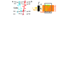
Figure 1: Schematic of wideband atomic slow light system. (a) The hyperfine structure of the $D_{1}$ line in ⁸⁷Rb. The bare energy levels are shown as dotted lines. The excited state splitting is $(2\pi)817$ MHz, the ground state splitting is $(2\pi)6.834$ GHz, and the $D_{1}$ optical transition is at $\lambda=795$ nm Steck . A magnetic field along the quantization axis ($z$) splits the individual Zeeman sub-levels $|i\rangle$ (solid black lines) according to $\Delta_{Z}^{(i)}=\mu_{B}g_{F}^{(i)}m_{F}^{(i)}B_{z}$ shown schematically in the figure for a positive magnetic field. We consider two EIT $\Lambda$ schemes (Scheme A as dashed arrows(blue online), Scheme B as solid arrows (red online)). The thicker arrows indicate the pump field, with frequency $\omega_{p}$ chosen to be resonant with the $\mbox{$|2\rangle$}\leftrightarrow\mbox{$|3\rangle$}$ transition with no magnetic field. The thinner arrows refer to the signal field, at some arbitrary frequency $\omega_{s}$ within our desired bandwidth. The magnetic field is chosen such so the system is in two-photon resonance. In each case the atoms are initially purely in $|1\rangle$. In Scheme A, the fields also couple to $\mbox{$|4\rangle$}=\mbox{$|F^{\prime}=2,m_{F}=-1\rangle$}$, causing a decoherence mechanism which we investigate. (b) The channelization architecture. A signal field is split, such that the $x$ position of each frequency component is proportional to the frequency, and then input into a cell illuminated by a monochromatic pump field. A magnetic field with a linear gradient (dotted arrows, green online) is then applied across the cell in such a way that two photon resonance is nearly maintained everywhere.

The need for a wide-band, controllable true-time delay device inspired us to here consider theoretically a “channelization” geometry utilizing Zeeman shifts in the atoms (see Fig.1(b)). There are a variety of techniques available to spatially separate various frequency components of broadband light. Assume a broadband signal pulse (represented as a dashed, yellow arrow) propagating along the longitudinal ($z$) dimension is split in the transverse ($x$) direction, with a transverse displacement proportional to the detuning from some chosen central frequency. In our channelization geometry, this dispersed signal then enters the ⁸⁷Rb cell, which is illuminated by a co-propagating, monochromatic pump field. When particular Zeeman sublevels are used, as in Fig.1(a), the two photon resonance condition required for slow light will be a strong function of magnetic field along the quantization axis $z$ due Zeeman shifts of the levels. Thus, applying a longitudinal magnetic field (dotted, green arrows) with a linear gradient along $x$ will allow us to achieve the conditions for EIT and USL for each frequency simultaneously. The components can then be recombined after passing through the cell, resulting in a true time delay device for a broadband signal.

USL is a group (rather than phase) velocity effect, meaning it works by applying differential phase shifts to each frequency component in the signal pulse. Maintaining perfect two-photon resonance everywhere would result in no differential phase shift and thus, no delay. Therefore, one should choose the magnetic field gradient such that there is a small, varying detuning across the cell. By choosing this mismatch to be small enough that all components are within the EIT resonance one can obtain the linear frequency dispersion necessary for slow light and still maintain transparency. There is a direct trade-off such that the delay-bandwidth product cannot be increased with this method. But for many applications, such as delays for signal processing, delays in conventional slow light systems are much longer than necessary, while the bandwidth is much too small. Our method allows one to circumvent this problem.

To be of practical interest, such a system would ideally provide uniform transmission and delay over the entire bandwidth. We will see that Doppler broadening due to thermal motion of a room temperature vapor is actually beneficial to our scheme in this respect. Two-photon resonance is maintained for atoms of all velocities because the two fields are co-propagating, while the one-photon detuning strongly depends on the velocity of each atom. Once one averages over the Doppler profile one finds that delay and transmission insensitive to the one-photon detuning when it is well within the Doppler width ($\sim$300 MHz in room temperature rubidium) onePhoton . This means that the one-photon detuning resulting from our Zeeman shifts (see Fig. 1(a)) does not effect our delays and transmissions.

There are several issues to consider to optimize the system we propose here. First, the transmission (and maximum delay) are limited by decay of the coherence between the two ground states. This decay time is often governed by the time it takes the atoms to leave the interaction region with the pump (due to thermal motion) slowThermal . This decoherence mechanism can be mitigated by the addition of a buffer gas (such as helium) bufferCoherence ; slowThermal ; Arimondo which significantly reduces the diffusion of the ⁸⁷Rb atoms via collisions. Second, decoherence can also occur from transitions to levels outside the $\Lambda$ system of interest (for example, the level $|4\rangle$ in Scheme A in Fig. 1(a)). The presence of a high pressure of buffer gas can actually worsen this problem by pressure broadening these unwanted levels. This means there is often an optimal intermediate pressure which balances these two considerations. A third consideration, unique to the channelization architecture, is the presence of a high magnetic field gradient. Because the two photon resonance condition is only satisfied over a small range of magnetic fields, and therefore a small transverse spatial region, the thermal diffusion of atoms will put them out of two-photon resonance and potentially cause a severe absorption of the signal. This will mean higher buffer gas pressures may be desirable for our proposal than in conventional slow light.

In this paper, we present calculations of the transparency, delays and bandwidths for both Schemes A and B in ⁸⁷Rb atoms with a helium buffer gas. We use a model based on the linear response of the signal in the medium, taking into account the diffusion of the atoms, the linear gradient of the magnetic field, pressure broadening, Doppler broadening, as well as interaction with additional levels in the hyperfine structure. The calculation uses a semi-classical model of the evolution of the ensemble average of the atomic density matrix interacting with classical light fields, and a classical treatment of the light field propagation based on the slowly varying envelope (SVE) version of Maxwell’s equations quantumOptics .

In the first part of the paper we consider the case of a spatially uniform (but arbitrary) magnetic field and present a systematic analysis and optimization of the transmission and delays (with regards to buffer gas pressure and ⁸⁷Rb density, etc.). In the second part, we then introduce a model to account for a magnetic field with a steep linear gradient. We then discuss how to best choose the slight mismatch in the two-photon resonance to maximize the delay-bandwidth product. We find that Scheme B, provides better overall performance, with delays $\sim$5 ns over a bandwidth $\sim$50 MHz. We find that the delay-bandwidth product decreases with bandwidth, reaching unity at around 50 MHz. However, it is more difficult to prepare the initial state for this scheme (all atoms in $|F=1,m_{F}=+1\rangle$) than it is for Scheme A (all atoms in $|F=2,m_{F}=-2\rangle$, which is easily initialized via optical pumping from the pump). While Scheme A provides worse overall performance, it should still provide a suitable system to improve the bandwidth over conventional systems.

II Uniform magnetic field case

We begin by analyzing “conventional” slow light slowCold ; stoppedThermal , with a homogenous magnetic field and attempt to understand the delays, bandwidths and delay-bandwidth products achievable in both schemes A and B. Our model accounts for effects of an extra level $|4\rangle$ and the buffer gas and can also explore the dependence on the magnetic field.

II.1 Model

We model the signal and pump light fields classically and represent them with Rabi frequencies $\Omega_{s(p)}\equiv-e\mathbf{r}_{13(23)}\cdot\hat{\epsilon}_{s(p)}E_{s(p)}/\hbar$, where $\mathbf{r}_{ij}$ are dipole matrix elements, $\hat{\epsilon}_{s(p)}$ are unit polarization vectors, and $E_{s(p)}$ are the slowly varying envelopes of the electric fields $E_{s(p)}(e^{i(k_{s(p)}z-\omega_{s(p)}t)}+c.c)/2$. Here the wavenumbers $k_{s},k_{p}\approx 2\pi/\lambda$, with $\lambda=795$ nm the wavelength, are taken to be equal. The field polarizations $\hat{\epsilon}_{s(p)}$ are chosen to match the transitions ($\sigma_{+},\sigma_{-}$ in Scheme A and $\sigma_{+},\sigma_{+}$ in Scheme B). Meanwhile the ⁸⁷Rb atoms are represented by a $4\times 4$ density matrix $\hat{\rho}^{0}$ (representing each internal level $|i\rangle$ under consideration). The diagonal elements represent the fractional populations in each state while the off-diagonal terms represent the coherences between levels (induced by the coherent lasers). At the microscopic level, each atom has a density matrix but we course grain average over spatial regions large compared to the inter-atomic spacing, meaning the total density matrix can be approximated by $N\hat{\rho}^{0}$, where $N$ is the atomic density and $\hat{\rho}^{0}$ is normalized to unity $\sum_{i}\rho^{0}_{ii}=1$.

Our model for the atomic density matrix evolution has two parts: (1) a coherent, Hamiltonian part, which includes coupling with the light fields, Zeeman shifts, and pressure shifts; and (2) an incoherent part, which includes spontaneous decay, pressure broadening, and diffusion out of the pump field interaction region (or the cell walls if the pump illuminates the entire cell). The evolution equations for the density matrix elements are given by:

$$\dot{\rho}_{ij}^{0} = -(i/\hbar)[\hat{\rho}^{0},\hat{\mathcal{H}}]_{ij}+\sum_{kl}\mathcal{L}^{ij}_{kl}\rho^{0}_{kl};$$ (1)

$$\mathrm{where}$$

$$\hat{\mathcal{H}} = \hbar\left(\begin{array}[]{cccc}\omega_{1}+\Delta_{Z}^{(1)}&0&\frac{1}{2}\Omega_{s}^{*}e^{-i(k_{s}z-\omega_{s}t)}&\frac{1}{2}\beta_{14}\Omega_{s}^{*}e^{-i(k_{s}z-\omega_{s}t)}\\ 0&\omega_{2}+\Delta_{Z}^{(2)}&\frac{1}{2}\Omega_{p}^{*}e^{-i(k_{p}z-\omega_{p}t)}&\frac{1}{2}\beta_{24}\Omega_{p}^{*}e^{-i(k_{p}z-\omega_{p}t)}\\ \frac{1}{2}\Omega_{s}e^{i(k_{s}z-\omega_{s}t)}&\frac{1}{2}\Omega_{p}e^{i(k_{p}z-\omega_{p}t)}&\omega_{3}+\Delta_{Z}^{(3)}+S_{p}^{(\mathrm{e})}p&0\\ \frac{1}{2}\beta_{14}\Omega_{s}e^{i(k_{s}z-\omega_{s}t)}&\frac{1}{2}\beta_{24}\Omega_{p}e^{i(k_{p}z-\omega_{p}t)}&0&\omega_{4}+\Delta_{Z}^{(4)}+S_{p}^{(\mathrm{e})}p\end{array}\right).$$ (6)

The parameters $\beta_{14(24)}=\hat{\epsilon}_{s(p)}\cdot\mathbf{r}_{14(24)}/\hat{\epsilon}_{s(p)}\cdot\mathbf{r}_{13(23)}$ characterize the difference in coupling (both sign and amplitude) for the unwanted transition to $|4\rangle$. They are given by ratios of Clebsch-Gordon coefficients and are $\beta_{14}=1/\sqrt{3},\beta_{24}=-\sqrt{3}$ for Scheme A Steck and vanish for Scheme B, where there is no coupling to additional levels. We have made the rotating wave approximation to eliminate counter-rotating terms and coupling to levels detuned by the ground-state hyperfine frequencies ($\sim 6.8$ GHz), but kept terms detuned only by the excited-state hyperfine detuning ($\sim 800$ MHz). The bare level frequencies $\omega_{j}$ on the diagonal terms are shifted by linear Zeeman shifts $\Delta_{Z}^{(i)}=\mu_{B}g_{F}^{(i)}m_{F}^{(i)}B_{z}$ where the Bohr magneton is $\mu_{B}=(2\pi)1.4~{}\mathrm{MHz/G}$, the Lande g-Factors $g_{F}^{(i)}$ are given in Fig. 1(a), and $B_{z}$ is the magnetic field Steck . They are also shifted by buffer gas pressure shifts $S_{p}^{(i)}p$, where $p$ is the pressure. For ⁸⁷Rb with a helium buffer gas, these are taken to be $S_{p}^{(\mathrm{e})}=-(2\pi)0.9$ MHz/Torr for all excited manifold ($F^{\prime}=1,F^{\prime}=2$) states expBuffer (the ground state pressure shifts are much smaller and negligible for our parameters).

The incoherent evolution is governed by a super-operator $\tilde{\mathcal{L}}$. Writing out only the non-zero terms:

$$\mathcal{L}^{11(22)}_{33} = +\Gamma_{r}f_{13(23)},\hskip 56.9055pt\mathcal{L}^{11(22)}_{44}=+\Gamma_{r}f_{14(24)},\hskip 56.9055pt\mathcal{L}^{33(44)}_{33(44)}=-\Gamma_{r}$$

$$\mathcal{L}^{12}_{12} = -\gamma_{\mathrm{diff}},\hskip 56.9055pt\mathcal{L}^{13(14)}_{13(14)}=-(\Gamma_{r}/2+B_{p}p),\hskip 56.9055pt\mathcal{L}^{34}_{34}=-(\Gamma_{r}+2B_{p}p)$$ (7)

(plus the corresponding complex conjugate terms for the off-diagonal elements). These terms are generally non-Hermitian as they involve lossy terms and incoherent transitions due to spontaneous emission. The first line represents feeding the ground states $\mbox{$|1\rangle$},\mbox{$|2\rangle$}$ via spontaneous emission from $\mbox{$|3\rangle$},\mbox{$|4\rangle$}$. The rate of emission from these levels is $\Gamma_{r}=(2\pi)6$ MHz but this can branch into both levels $\mbox{$|1\rangle$},\mbox{$|2\rangle$}$ as well as other levels outside of the system of interest. The branching ratios to various states are given by the oscillator strengths $f_{ij}$ which are proportional to the square of the Clebsch-Gordon coefficients. For Scheme A, $f_{13}=1/2,f_{23}=1/12$ and $f_{j4}=|\beta_{j4}|^{2}f_{j3}$, while for Scheme B, $f_{13}=1/2,f_{23}=1/6$. The second line represents the population loss of the excited states from spontaneous emission. In the third line, we have put in the dephasing of the ground state coherence due to the diffusion of the gas out of the interaction region (taken to be of width $w_{\mathrm{int}}$ and height $h_{\mathrm{int}}$) Arimondo :

$$\gamma_{\mathrm{diff}}=\frac{2}{3}2.405^{2}\frac{D_{g}}{w_{\mathrm{int}}h_{\mathrm{int}}}\frac{1}{1+6.8\,l_{\mathrm{mfp}}/\sqrt{w_{\mathrm{int}}h_{\mathrm{int}}}},$$ (8)

where the diffusion constant for ⁸⁷Rb in a helium buffer gas of pressure $p$ and temperature $T$ is
$D_{g}=(410~{}\mathrm{cm^{2}/s})(\mathrm{Torr}/p)\sqrt{T/273~{}\mathrm{K}}$ Happer . The mean free path is $l_{\mathrm{mfp}}=3D_{g}/v_{th}$ and the thermal velocity $v_{th}=\sqrt{3k_{B}T/m}$. The factor (2/3) in front is to account for the fact that length (along $z$) is generally much longer than $w_{\mathrm{int}},h_{\mathrm{int}}$ and diffusion in this dimension does not effect the coherence. There is additionally a depolarizing cross-section from ⁸⁷Rb-He collisions, which can dephase the ground states, but this is much smaller effect than other decoherence mechanisms for our parameters of interest and is neglected. The last two lines of Eq. (II.1) contain dephasings of coherences from radiation, at $\Gamma_{r}/2$, and pressure broadening, with $B_{p}=(2\pi)$5 MHz/Torr expBuffer ; bufferAbs .

When solving Eq. (1), we consider the usual weak signal regime, and drop all terms higher than linear order in $\Omega_{s}$. This is valid when $|\Omega_{s}|\ll|\Omega_{p}|$ and when multiple scattering of spontaneously emitted photons can be ignored (which is usually the case in EIT since spontaneous emission is suppressed). Then we can take $\rho^{0}_{11}\rightarrow 1$ and $\rho^{0}_{22},\rho^{0}_{33},\rho^{0}_{44},\rho^{0}_{23},\rho^{0}_{24},\rho^{0}_{34}\rightarrow 0$. We are left with three non-trivial equations for the evolution of $\rho^{0}_{21},\rho^{0}_{31},\rho^{0}_{41}$. We furthermore make transformations to eliminate the time-dependent terms in Eq. (6): $\rho_{31,41}=\rho^{0}_{31,41}e^{-i(k_{s}z-\omega_{s}t)},\rho_{21}=\rho^{0}_{21}e^{-i((k_{s}-k_{p})z-(\omega_{s}-\omega_{p})t)}$. For convenience we define a vector $\mathbf{\rho}\equiv[\rho_{21},\rho_{31},\rho_{41}]^{T}$. The evolution Eq. (1) can then be written as:

$$\dot{\mathbf{\rho}} = \hat{\mathcal{M}}\mathbf{\rho}+\mathbf{S};$$

$$\hat{\mathcal{M}} \equiv \left(\begin{array}[]{ccc}i(\Delta_{s}^{\prime}-\Delta_{p}^{\prime})-\gamma_{\mathrm{diff}}&-\frac{i}{2}\Omega_{p}^{*}&-\frac{i}{2}\beta_{24}\Omega_{p}^{*}\\ -\frac{i}{2}\Omega_{p}&i(\Delta_{s}^{\prime}+\delta_{D})-\gamma_{e}&0\\ -\frac{i}{2}\beta_{24}\Omega_{p}&0&i(\Delta_{s}^{\prime}-\Delta_{43}^{\prime}+\delta_{D})-\gamma_{e}\end{array}\right),$$

$$\mathbf{S} \equiv (0,-\frac{i}{2}\Omega_{s},-\frac{i}{2}\beta_{14}\Omega_{s})^{T}$$ (12)

where we have defined the shifted detunings, $\Delta_{s}^{\prime}=\Delta_{s}-\Delta_{Z}^{(3)}-S_{p}^{(\mathrm{e})}p+\Delta_{Z}^{(1)},\,\Delta_{p}^{\prime}=\Delta_{p}-\Delta_{Z}^{(3)}-S_{p}^{(\mathrm{e})}p+\Delta_{Z}^{(2)}$, and $\Delta_{43}^{\prime}=\omega_{4}^{(0)}+\Delta_{Z}^{(4)}-\omega_{3}^{(0)}-\Delta_{Z}^{(3)}$. The bare detunings are $\Delta_{s(p)}=\omega_{s(p)}-(\omega_{3}-\omega_{1(2)})$. Throughout we choose pump to resonant with the bare resonance $\Delta_{p}=0$, while the signal $\Delta_{s}$ varies. We have also introduced a Doppler shift $\delta_{D}=(2\pi)v_{z}/\lambda$, where $v_{z}$ is the velocity of a particular atom along the light propagation direction $z$. The total dephasing rates of the optical transitions are $\gamma_{e}=\Gamma_{r}/2+B_{p}p$.

When studying the light field propagation, it will be easiest to work in Fourier space and so we transform from $\mathbf{\rho}(t)\rightarrow\bar{\mathbf{\rho}}(\delta)$ and $\Omega_{s}(t)\rightarrow\bar{\Omega}_{s}(\delta)$. Equation (II.1) is linear in time-dependent quantities and finding the solution of its Fourier transform is equivalent to solving for its steady state in the time domain but replacing $\Delta_{s}\rightarrow\bar{\Delta}_{s}=\Delta_{s}+\delta$ where $\delta$ represents the deviation of a particular Fourier component of the signal field $\bar{\Omega}_{s}$ from the central probe frequency $\omega_{p}$ (due to time dependence). This solution is:

$$\bar{\mathbf{\rho}}=\hat{\bar{\mathcal{M}}}^{-1}\mathbf{\bar{S}},$$ (13)

where $\hat{\bar{\mathcal{M}}}^{-1}$ is simply $\hat{\mathcal{M}}^{-1}$ after making the replacement $\Delta_{s}\rightarrow\bar{\Delta}_{s}$ and in $\mathbf{\bar{S}}$ we replace $\Omega_{s}\rightarrow\bar{\Omega}_{s}$.

Finally, to obtain the response of the entire medium we integrate over the thermal profile of velocities $v_{z}$ slowThermal :

$$\bar{\rho}^{(D)}(\bar{\Delta}_{s})=\int d\delta_{D}\,\bar{\rho}(\bar{\Delta}_{s},\delta_{D})\,\mathrm{exp}\bigg{(}-\frac{\delta_{D}^{2}}{\Delta_{D}^{2}}\bigg{)},$$ (14)

where the Doppler width is $\Delta_{D}=\sqrt{2/3}(2\pi)v_{th}/\lambda$ (the square root term is a geometrical factor).

Turning now to the light propagation, in the linear signal regime the pump field Rabi frequency $\Omega_{p}$ is constant in space and time. The signal field $\Omega_{s}$ propagates according to the SVE Maxwell equation, with the polarization written in terms of the atomic density matrix. Once we Fourier transform the Maxwell equation, it can be written:

$$\frac{\partial}{\partial z}\bar{\Omega}_{s} = \frac{i}{2}Nf_{13}\sigma\chi^{(D)}(\bar{\Delta}_{s})\bar{\Omega}_{s}+i\frac{\delta}{c}\bar{\Omega}_{s}$$

$$\mathrm{where}\hskip 28.45274pt\chi^{(D)}(\bar{\Delta}_{s}) = -\frac{\Gamma_{r}}{\bar{\Omega}_{s}}(\bar{\rho}_{31}^{(D)}+\beta_{14}\bar{\rho}_{41}^{(D)})$$ (15)

and $\sigma=3\lambda^{2}/(2\pi)$ is the resonant cross section for unity oscillator strength. The last term accounts for the propagation at $c$ in free space. If the fastest time scale of interest in the problem is much slower than total length of propagation ($\sim$ cm) divided by $c$ then this term can be neglected. Note that since $\bar{\rho}_{31},\bar{\rho}_{41}\propto\bar{\Omega}_{s}$, the susceptibility is independent of $\bar{\Omega}_{s}$. Equation (II.1) can be trivially solved to give how a particular frequency component, with an input amplitude $\bar{\Omega}_{s}^{(\mathrm{in})}(\bar{\Delta}_{s})$, will propagate through a cell of length $l_{\mathrm{cell}}$ in the medium $\bar{\Omega}_{s}^{(\mathrm{out})}(\bar{\Delta}_{s})=e^{\frac{i}{2}D\chi^{(D)}(\bar{\Delta}_{s})}\bar{\Omega}_{s}^{(\mathrm{in})}(\bar{\Delta}_{s})$, where the “optical density” is defined as $D=f_{13}N\sigma l_{\mathrm{cell}}$ (we have ignored the speed of light propagation term for simplicity). From this one clearly sees how the imaginary part of $\chi^{(D)}$ is proportional to the absorption cross-section while the real part is gives phase shifts and thus determines the index of refraction.

In a non-Doppler broadened, non-pressure broadened medium in the absence of a pump field ($\Omega_{p}\rightarrow 0$), and with no level $|4\rangle$ ($\beta_{14}=0)$, we recover the usual Lorentzian susceptibility profile. The absorption cross-section is peaked at the atomic resonance $\Delta_{s}^{\prime}=0$ and has a width $\Gamma_{r}$ while the real part exhibits anomalous dispersion at the resonance. The dimensionless susceptibility $\chi^{(D)}$ in Eq. (II.1) has been defined such that the peak absorption is $\chi^{(D)}(\Delta_{s}^{\prime}=0)=i$, leading to exponential attenuation of the signal intensity $I_{s}\propto e^{-D}$. Pressure broadening and Doppler broadening act to reduce this resonant cross section while widening the feature.

II.2 Results

The presence of a sufficiently strong pump field $\Omega_{s}$ will then introduce a sharp EIT feature at frequencies very near the two-photon resonance, in the middle of this broad absorption resonance. At the EIT resonance, we have reduced absorption (transparency) and a linear slope in the index of refraction with normal (positive) dispersion (leading to the slow group velocity). We now proceed with some calculations of these EIT features. The primary motivation of the present section is to learn the role played by the buffer gas pressure and to quantitatively learn the dependence on magnetic field. These results will later guide the optimization of the channelization architecture with the linear magnetic field gradient.

Throughout this section consider a case with a 1 mW pump laser with an area $w_{\mathrm{int}}h_{\mathrm{int}}=(2~{}\mathrm{mm})^{2}$. Due to differing oscillator strengths $f_{23}$ this results in Rabi frequencies of $\Omega_{p}=(2\pi)8.45$ MHz for Scheme A and $\Omega_{p}=(2\pi)12.3$ MHz for Scheme B. At a temperature of $T=333$ K (60 degrees Celcius), there is a ⁸⁷Rb density of $N=2.5\times 10^{11}~{}\mathrm{cm}^{-3}$ Steck and a Doppler width $\Delta_{D}=(2\pi)320$ MHz.

Considering first a homogenous $B_{z}=0$ magnetic field, we plot in Fig.2 the real and imaginary parts of the Doppler averaged susceptibility $\chi_{R}^{(D)}(\bar{\Delta}_{s}),\chi_{I}^{(D)}(\bar{\Delta}_{s})$, according to Eq. (II.1), both on a large (a,b) and small (c,d) scale for both Schemes A (thinner, blue curves) and Scheme B (thicker, red curves). From Fig.2(a,b) we see that, away from the narrow EIT feature, the susceptibility retains the usual Lorentzian susceptibility feature one would expect in a two-level medium, with the width $\sim\Delta_{D}$ and height $\sim\Gamma_{r}/2\Delta_{D}$. The biggest apparent difference between the two schemes is that in Scheme A there is an extra resonance, due to level $|4\rangle$, near the hyperfine splitting ($\sim 817$ MHz). Note that we are in a regime where the Doppler broadening is comparable to this splitting, causing the two resonances to slightly overlap. The solid curves are for the relatively small buffer gas pressure $p=3$ Torr, while the dotted curves are for $p=30$ Torr. At this higher pressure, the pressure broadening becomes important as $\gamma_{e}=(2\pi)~{}253$ MHz becomes comparable to $\Delta_{D}$.

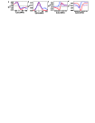
Figure 2: EIT transparency window and steep index of refraction. (a-b) Frequency dependence of the real (a) and imaginary (b) parts of the susceptibility $\chi^{(D)}$ in Schemes A (thin curves, red online) and B (thick curves, blue online) with $B_{z}=0$. Buffer gas pressures are p=3 Torr (solid curves) and 30 Torr (dotted curves). The scale is too large to see the EIT resonance features, which is located at the vertical dotted lines. (c-d) The same curves shown on a smaller scale, at the EIT resonance. The dotted lines indicate exact two-photon resonance $\Delta_{p}^{\prime}=\Delta_{c}^{\prime}$.

Examining the smaller scale plots Fig. 2(c-d), we see the pump field introduces a sharp feature at the two-photon resonance ($\bar{\Delta}_{s}=0$). In the imaginary part we see a narrow notch in the absorption cross-section (the transparency window) while in the real part we see steep linear dispersion, the origin of the slow group velocity. To describe the degree of transparency, we define the parameter $R_{\mathrm{EIT}}$ as the ratio of the minimum of $\chi_{I}^{(D)}(\bar{\Delta}_{s})$ in the resonance to its value there with no pump field present. We note a very large difference in this parameter for the two schemes, with only $R_{\mathrm{EIT}}\approx 1/3$ for Scheme A. As we will discuss below, coupling to level $|4\rangle$ is the reason for the lack of good transparency in this case. We also note that the transparency window is slightly shifted from exact two photon resonance (by approximately $-0.1~{}$MHz), an effect of stark shifts from $|4\rangle$. In Scheme B, the transparency is quite good $R_{\mathrm{EIT}}\sim 0.001$.

To translate these $\chi^{(D)}(\bar{\Delta}_{s})$ curves into performance for delay devices, we examine the shape of these curves at the EIT resonance. To a good approximation, the real part here can be written as some central value plus a linear part, while the imaginary part is some minimum value plus a parabolic shape:

$$\chi^{(D)}(\bar{\Delta}_{s})\approx\phi_{0}+S(\bar{\Delta}_{s}-\Delta_{0})+iA+i\frac{(\bar{\Delta}_{s}-\Delta_{0})^{2}}{W^{2}}$$ (16)

where $\Delta_{0}$ is defined to be the minimum point of $\chi_{I}^{(D)}$ and the parameters $\phi_{0},\,A\,\mathrm{absorption}\,S\,\mathrm{(slope)},\,W\,\mathrm{(width)}$ are obtained by numerically evaluating $\chi^{(D)}(\bar{\Delta}_{s})$ and its derivatives at $\Delta_{0}$. In these terms our transparency parameter is $R_{\mathrm{EIT}}=A/\mathrm{Im}\{\chi^{(D)}(\Delta_{0})|_{\Omega_{p}\rightarrow 0}\}$.

Now suppose we input a signal pulse a central frequency $\Delta_{s}=\Delta_{0}$ and a $1/e$ intensity half-width $\tau_{s}$ (giving it frequency components in the range $\bar{\Delta}_{s}=\Delta_{0}\pm\tau_{s}^{-1}$). To calculate what the pulse looks like after propagation through the medium, one takes the Fourier transform of the input pulse, calculates the propagation of each Fourier component according to Eq. (II.1), then inverts the Fourier transformation back to the time domain. If $\tau_{s}$ sufficiently long that Eq. (16) is valid for all frequency components of the pulse (which is usually true when $\tau_{s}^{-1}\ll W$), then one can analytically perform the inverse transformation. The result is a pulse which is delayed in time by $\tau_{D}=DS/2$ and attenuated by a factor $e^{-AD}$. This Fourier analysis of the propagation reveals clearly how the delay comes about by a differential phase shift of the different frequency components $S\Delta_{s}^{\prime}D/2$. One immediately sees there is a trade-off between transparency and delay. In addition, frequency components slightly off the resonance will be preferentially absorbed. This leads to a time-broadening of the pulse by $\tau\rightarrow\sqrt{\tau_{s}^{2}+\beta^{-2}}$, where $\beta=W/\sqrt{D}$, and a reduction in the peak intensity by $\tau^{2}/(\tau_{s}^{2}+\beta^{-2})$. In this sense, $\beta$ can be interpreted as the bandwidth of the system, as $\delta\sim\tau_{s}^{-1}\ll\beta$ is required to prevent attenuation and distortion of the pulse.

An obvious figure of merit is the delay-bandwidth product, important for many applications such as quantum memory devices or optical buffers. This parameter indicates the degree of “pulse separation” one can achieve (i.e. the number of pulse widths one can delay). Incidentally, this parameter being unity corresponds to the point at which the differential phase shifts across the frequency spectrum of the pulse is $\sim(2\pi)$. However, the absolute value of the bandwidth and maximum delay are also of importance, depending on the application. All these parameters depend strongly on the optical density $D$, which can generally be adjusted since the ⁸⁷Rb density $N$ is a strong function of temperature Steck . At $N=2.5\times 10^{11}~{}\mathrm{cm}^{-3}$ for a $l_{\mathrm{cell}}=1$ cm cell, $D=370$. For a given desired transmission, the parameter $A$ tells us the optical density through which a pulse can successfully propagate. For a transmission $1/e$ we need $D<D_{\mathrm{max}}=A^{-1}$. This, in turn, determines the maximum achievable delay $\tau_{D}^{\mathrm{(max)}}=S/2A$. The delay-bandwidth product is $\tau_{D}\beta=SW\sqrt{D}/2$. This product increases with $D$ and the best possible delay-bandwidth (using $D_{\mathrm{max}}$) is $SW/2\sqrt{A}$.

For Scheme A we find the performance is better for lower pressures. At $p=2$ Torr and other parameters as in Fig. 2, we calculate $A=0.005$, $S=24$ ns and $W=(2\pi)0.72$ MHz, giving a maximum delay-bandwidth product of 0.76. In Fig. 3(a), we plot resulting pulse propagation parameters versus $D$. We see that for $D\approx 50$ one obtains a $\tau_{D}=0.5~{}\mu$s delay with only 20% loss. But the minimum pulse width here is $\beta^{-1}=1.5~{}\mu\mathrm{s}>\tau_{D}^{\mathrm{max}}$ One does not get into the “pulse separation” regime until at about $D=350$, where $\tau_{D}=\beta^{-1}=4.1~{}\mu$s where the attenuation is 82% and the bandwidth is $\beta=(2\pi)38$ kHz.

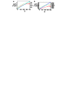
Figure 3: Pulse propagation characteristics (a) For the case $p=2$ Torr, $B_{z}=0$ in Scheme A we calculate $A=0.005,\,S=24~{}\mathrm{ns}$, and $W=(2\pi)0.72$ MHz. Here we plot the resulting delay $\tau_{D}=SD/2$ (solid curve, blue online), loss $L=(1-e^{-AD}))$ (dashed, red) and inverse bandwidth $\beta^{-1}=\sqrt{D}/W$ (dotted, green) versus optical density $D$. (b) Same for Scheme B, with $p=15$ Torr, for which $A=3.5\times 10^{-5}$, $S=13.3$ ns, and $W=(2\pi)2.31$ MHz.

By contrast, we can do much better in Scheme B. We find this system is better at higher pressures and for $p=15$ Torr case we calculate $A=3.5\times 10^{-5}$, $S=13.3$ ns, and $W=(2\pi)2.31$ MHz, giving $\beta\tau_{D}^{\mathrm{(max)}}=31$. The pulse propagation parameters are plotted in Fig. 3(b) and we see the pulse separation regime begins at $D\approx 100$, at which point $\tau_{D}\approx 0.7~{}\mu$s and the loss is only $L\approx 0.003$. The bandwidth here is $\beta=(2\pi)230$ kHz. Note that despite the better performance, one would still have to go to very small $D$ to get the bandwidth significantly more than 1 MHz, and here the delay-bandwidth product is quite small.

We now attempt to get some intuitive understanding of what determines $A,\,S$, and $W$ in the two schemes and study the dependence on buffer gas pressure and magnetic field. Scheme B, because of the absence of level $|4\rangle$ is significantly easier to understand. One can analytically obtain the solution Eq. (13) and plug it directly into the susceptibility in Eq. (II.1)). The conditions necessary for EIT are that the ground state decoherence rate is small $\gamma_{\mathrm{diff}}\ll\gamma_{e}$ and the pump field intensity is sufficiently strong $|\Omega_{p}|^{2}\gg\gamma_{\mathrm{diff}}\gamma_{e}$. Assuming these inequalities and Taylor expanding in $\bar{\Delta}_{s}^{\prime}$ about one- and two-photon resonance ($\bar{\Delta}_{s}^{\prime}=\Delta_{p}^{\prime}=0)$ one obtains a susceptibility in the form of Eq. (16) with the parameters $\phi_{0}=0,\,A=2\gamma_{\mathrm{diff}}\Gamma_{r}/|\Omega_{p}|^{2},\,S=2\Gamma_{r}/|\Omega_{p}|^{2},\,W=|\Omega_{p}|^{2}/\sqrt{8\gamma_{e}\Gamma_{r}}$. Thus we find that the absorption scales as the inverse of the pump intensity, the bandwidth scales directly with the intensity and the delay scales inversely with the intensity. There is a trade-off between delay and attenuation in choosing the pump intensity (just like the optical density). However, unlike with optical density, one cannot improve the delay-bandwidth product by changing the pump intensity. One can increase the bandwidth (and reduce the delay) but extremely high bandwidths require unreasonably high pump powers. We find that these analytic expressions are still valid after Doppler averaging. For the case we have just considered (Fig. 3(b)) these estimates yield $A=3.5\times 10^{-5},S=13.3~{}\mathrm{ns},W=(2\pi)2.34$ MHz, in excellent agreement with the numerical results.

At the point of transparency we find the ground state coherence is $\rho_{21}\approx-\Omega_{s}/\Omega_{p}$, which is known as a “dark state” EIT . The strong pump field acts to drive the system into this state. In this case the two terms driving absorption, on the $\mbox{$|1\rangle$}\leftrightarrow\mbox{$|3\rangle$}$ and $\mbox{$|2\rangle$}\leftrightarrow\mbox{$|3\rangle$}$ transitions, (see the first two terms on the third line of the Hamiltonian, Eq. (6)), are equal and opposite, leading to a quantum interference which suppresses the absorption process. However, a non-zero detuning $\Delta_{p}^{\prime}$ or decoherence $\gamma_{\mathrm{diff}}$ causes $\rho_{21}$ to slowly evolve out of the dark state. Our analytic expression $A=2\gamma_{\mathrm{diff}}\Gamma_{r}/|\Omega_{p}|^{2}$ reflects the steady-state which occurs due to the balance of the preparation of the dark state by the pump field and the loss from it due to diffusion. To minimize our absorption, we clearly want to minimize $\gamma_{\mathrm{diff}}$, which can be done by increasing the buffer gas pressure (which decreases $D_{g}$) or increasing the effective area of interaction $h_{\mathrm{int}}\times w_{\mathrm{int}}$ (see Eq. (8)). In practice, there is a trade-off between the interaction area and $|\Omega_{p}|^{2}$ as one can increase the pump intensity by focusing the it more tightly. Thus, for a given pump power and buffer gas pressure, there is only a marginal dependence of $A$ on the focusing area. Numerically we fine that there is a slight benefit in tighter focusing. Regardless one can increase the pressure to improve $A$ to the desired level. The slope $S$ is almost completely unaffected by $p$, while $W$ decreases with pressure due to the factor $\sqrt{\gamma_{e}}$ in the denominator.

For Scheme A, the situation is significantly altered by the presence of $|4\rangle$. The problem is that the dark state with respect to absorptions into $|3\rangle$ (the state for which the two absorption channels have equal and opposite amplitudes) is $\rho_{21}=-\Omega_{s}/\Omega_{p}$ while the dark state with respect to $|4\rangle$ is $\rho_{21}=-\beta_{14}\Omega_{s}/\beta_{24}\Omega_{p}$. Thus, unless oscillator strength ratios are equal $\beta_{14}=\beta_{24}$ there will be some absorption present for any value of $\rho_{21}$. In Scheme A, $\beta_{14}=1/\sqrt{3}$ and $\beta_{24}=-1\sqrt{3}$.

This problem was studied in detail for the cold atom (non-Doppler broadened) case in thesis . There it was found that, for atoms nearly resonant with $|3\rangle$, this effect leads to minimum absorption coefficient $A_{\mathrm{off-res}}=(\beta_{14}-\beta_{24})^{2}\gamma_{e}\Gamma_{r}/4(\Delta_{43}^{\prime 2}+\gamma_{e}^{2})$ and an AC Stark shift of the EIT resonance by $\Delta_{\mathrm{AC}}=\beta_{24}(\beta_{24}-\beta_{14})|\Omega_{p}|^{2}\gamma_{e}/4(\Delta_{43}^{\prime 2}+\gamma_{e}^{2})$. In the Doppler broadened case this problem is further complicated by the fact that, when the Doppler width $\Delta_{D}$ is comparable to the hyperfine splitting $\Delta_{43}^{\prime}$, there is a significant fraction of atoms which interact with both $|3\rangle$ and $|4\rangle$ with similar strength. The EIT interference is almost completely destroyed for these atoms. Numerically, we find that for Scheme A, this increases $A_{\mathrm{off-res}}$ by nearly an order of magnitude from the analytic estimate above. Increasing pump power increases the coupling to $|4\rangle$ in such a way that it exactly offsets any gain in the strength of the EIT resonance, and so we find $R_{\mathrm{EIT}}$ quickly saturates to a value around 0.3 (as in Fig. 2(c-d)), a constant determined by the relative values of $\Delta_{D}$ and $\Delta_{43}^{\prime}$. The interesting thing to note about $A_{\mathrm{off-res}}$ is that it increases with buffer gas pressure (via $\gamma_{e}$) because pressure broadening increases the relative role played by coupling to $|4\rangle$. Therefore, the diffusion problem favors higher $p$, while the interaction with $|4\rangle$ generally favors lower pressure and the lowest overall absorption is achieved by balancing these two considerations. We find that the optimal pressure is rather low (between 0.5 - 2 Torr, depending on interaction area), but that the dependence is rather weak and so $R_{\mathrm{EIT}}\approx 0.3$ is a good estimate over a broad range of pressures and interaction areas. The AC Stark shift is visible in the plots Fig. 2(c-d) and agrees well with the above expression.

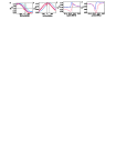
Figure 4: EIT in a homogenous magnetic field. Plot of $\chi^{(D)}$ in the two schemes, again for $p=3$ Torr. The solid curves are for $B_{z}=0$ (identical to Fig. 2), while the dotted curves are with a magnetic field $B_{z}=75$ G, which shifts the two-photon resonance ($\Delta_{s}^{\prime}=\Delta_{p}^{\prime}$) to $s_{\mathrm{res}}B_{z}=(2\pi)105$ MHz.

Finally, in preparation for our channelization calculations, we must consider the degree to which our results depend on the value of the homogenous magnetic field $B_{z}$. We still choose our pump field to be resonant with the bare $\mbox{$|2\rangle$}\leftrightarrow\mbox{$|3\rangle$}$ transition $\Delta_{p}=\omega_{p}-(\omega_{3}-\omega_{2})=0$. This system will then be in two-photon resonance for a probe photons with bare detuning $\Delta_{s}=\Delta_{Z}^{(2)}-\Delta_{Z}^{(1)}-\Delta_{\mathrm{AC}}=s_{\mathrm{res}}B_{z}-\Delta_{\mathrm{AC}}$, where $s_{\mathrm{res}}\equiv\mu_{B}(g_{F}^{(2)}m_{F}^{(2)}-g_{F}^{(1)}m_{F}^{(1)})$. In both Schemes A and B $s_{\mathrm{res}}=(2\pi)1.4$ MHz/G. In Fig. 4 we plot $\chi^{(D)}$ for both $B_{z}=0$ (solid curves) (as in Fig. 2) and with a large magnetic field $B_{z}=75$ G (dotted curves). In Fig. 4(a-b) we see that the magnetic field shifts the overall one-photon detuning so the Doppler broadened Lorentzian resonances are shifted. It also shifts the two-photon resonance (vertical lines) by a slightly different amount (so the EIT resonance with $B_{z}=75$ G is not exactly at peak of the Lorentzian resonance). However, this difference is still well within the Doppler width. Examination of the $g_{F}$ and $m_{F}$ shows that the signal detuning from $|3\rangle$, $\Delta_{s}^{\prime}$, (see Eq. (II.1) and below) is only $1/6$ of that of the two-photon resonance shift $s_{\mathrm{res}}B_{z}$ (this is true in both Schemes A and B, though the relative sign of the shift for the two schemes is opposite). Thus, even a shift of the two-photon resonance $s_{\mathrm{res}}B_{z}\sim\Delta_{D}$ will result in substantially smaller one-photon detuning. This is beneficial as the widths and strengths of the EIT resonances are effected when the one-photon detuning becomes comparable to the Doppler width onePhoton . Comparison of plots of the EIT resonance in Fig. 4(c-d) with the $B_{z}=0$ case in Fig. 2(c-d) reveals they looks almost identical.

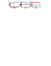
Figure 5: Dependence of EIT resonance on magnetic field. The parameters $A$ (a) $S$ (b) and $W$ (c) , versus magnetic field $B_{z}$. For Scheme A (thinner, blue), the pressure is $p=1.2$ Torr, and for Scheme B (thicker, red) $p=30$ Torr.

To check numerically that the EIT resonance is indeed insensitive to $B_{z}$ over a wide range, we calculated the parameters $A,S$ and $W$ over the range $B_{z}=$-200 G to +200 G. The results, presented in Fig. 5 bear out our expectation. In Scheme B there is no visible dependence on $B_{z}$ on the scale plotted. There is a weak dependence in the parameters in Scheme A, again primarily due to the effect of level $|4\rangle$. The total range of resonance frequencies for this range of magnetic fields is $(2\pi)560$ MHz.

III EIT and slow light with a magnetic field gradient

We are now prepared to add a final piece of our model account for the large gradients in the magnetic field and the transverse spatial dispersion of the signal in the proposed channelization geometry. We will then use this to characterize the performance of the delay device in each scheme, and explore quantitatively the maximum delays versus bandwidth and the optimal buffer gas pressures.

III.1 Model

Let us first consider how the susceptibility is affected by the diffusion of the gas in the presence of a magnetic field gradient. When a gas diffuses with some diffusion constant, it’s density matrix evolves as $\dot{\rho}=\cdots+D_{g}\nabla^{2}\rho$ Steck so we add this term to our existing evolution equation. Since the magnetic field gradient only exists in the $x$ dimension, the diffusion in $y$ and $z$ has no effect. We then write Eq. (II.1):

$$\dot{\mathbf{\rho}}=\hat{\mathcal{M}}\mathbf{\rho}+\mathbf{S}+\frac{D_{g}}{3}\frac{d^{2}}{dx^{2}}\mathbf{\rho}.$$ (17)

With a magnetic field gradient our shifted detunings $\Delta_{s}^{\prime},\Delta_{p}^{\prime}$ becomes spatially dependent and we take $\frac{d^{2}}{dx^{2}}\mathbf{\rho}\rightarrow(\frac{dB_{z}}{dx})^{2}\frac{\partial^{2}}{\partial B_{z}^{2}}\mathbf{\rho}$. Suppose we apply a linear gradient so $B_{z}(x)=S_{B}x$ over the interaction region of width $w_{\mathrm{int}}$. Then the two-photon resonance would vary by $\beta_{\mathrm{eff}}\equiv S_{B}w_{\mathrm{int}}s_{\mathrm{res}}$ over the width of the interaction region, determining the effective bandwidth of our system .

Our susceptibility in the presence of diffusion will then be the steady state solution of Eq. (17). It is difficult to find this analytically in general, but this can be achieved with a perturbation approach under the assumption that the new diffusion term is small. In the perturbative approach, we take a zeroeth order solution $\mathbf{\bar{\rho}}^{(0)}$ to be solution without the diffusion term $\mathbf{\bar{\rho}}^{(0)}=\hat{\mathcal{\bar{M}}}^{-1}\mathbf{\bar{S}}$ (see Eq. (13)), and then plug this back into the full equation to obtain a correction from the diffusion term:

$$\mathbf{\bar{\rho}^{(1)}}=S_{B}^{2}\frac{D_{g}}{3}\hat{\mathcal{M}}^{-1}\frac{\partial^{2}}{\partial B_{z}^{2}}\mathbf{\bar{\rho}}^{(0)}$$ (18)

Because the two-photon detuning $\Delta_{s}^{\prime}-\Delta_{p}^{\prime}$ is directly proportional to $B_{z}$, the second derivative with respect to the $B_{z}$ basically corresponds to the curvature with frequency of $\chi^{(D)}$ at the EIT resonance, which Eq. (16) predicts to be $2/W^{2}$. In a sense, the diffusion term causes an averaging over some frequency width, which will partly wash out the EIT resonance, increasing our minimum absorption $A$. It also has a tendency to widen the feature, increasing $W$ and decreasing our $S$.

After obtaining our corrected density matrix $\mathbf{\bar{\rho}}=\mathbf{\bar{\rho}^{(0)}}+\mathbf{\bar{\rho}^{(1)}}$ we once again Doppler average according to Eq. (14) and then calculate the susceptibility. Unfortunately, the perturbative procedure is not valid near the wings of the Doppler profile, where the EIT feature becomes very narrow, even in cases where the perturbation is small near the center of the Doppler profile. In the limit that the diffusion correction becomes large $\mathbf{\bar{\rho}}$ should smoothly return to it’s value without the EIT feature $\mathbf{\bar{\rho}}|_{\Omega_{p}\rightarrow 0}$, but in Eq. (18) the correction $\bar{\rho}^{(1)}$ can grow without bound. For this reason, we must use a slightly more complicated procedure, which in the limit of a small diffusion term reproduces Eq. (18) and in the opposite limit reverts to $\mathbf{\bar{\rho}}|_{\Omega_{p}\rightarrow 0}$. This is accomplished by taking an average over a small range of magnetic fields:

$$\mathbf{\bar{\rho}}(\bar{\Delta}_{s},\delta_{D},B) = \int d\delta_{B}\frac{1}{\sqrt{\pi}\Delta_{B}}\mathbf{\bar{\rho}^{(0)}}(\bar{\Delta}_{s},\delta_{D},B_{z}+\delta_{B})\mathrm{Exp}\bigg{(}-\frac{\delta_{B}^{2}}{\Delta_{B}^{2}}\bigg{)}$$

$$\mathrm{where}\hskip 28.45274pt\Delta_{B}^{2} = \frac{4D_{g}S_{B}^{2}}{3}\bigg{|}\frac{\sum_{j}\lambda_{j}a_{j}\mathbf{v}_{j}}{\sum_{j}\lambda_{j}\mathbf{v}_{j}}\bigg{|},$$ (19)

and the $\{\lambda_{j}\}$ and $\{\mathbf{v}_{j}\}$ are, respectively, the eigenvalues and eigenvectors of $\hat{\bar{\mathcal{M}}}^{-1}$ and the ${a_{j}}$ are the coefficients $a_{j}=\mathbf{v}_{j}\cdot(\partial^{2}\mathbf{\bar{\rho}}^{(0)}/\partial B_{z}^{2})$. After calculating Eq. (III.1) we can then Doppler average with Eq. (14).

Figure 6: Schematic of detunings in wideband slow light scheme. The signal pulse frequencies are dispersed along $x$ with a slope $S_{\mathrm{disp}}$, indicated by the black solid arrow, which is slightly larger than the slope of the two-photon resonance $S_{B}s_{\mathrm{res}}$, indicated with the dashed arrow. The values chosen for the mismatch in slopes is such that the detuning local resonance $\Delta_{p}^{\prime}$ varies linearly with $x$ and is everywhere within the local bandwidth $\beta$. The top row diagrams this mismatch with respect to the local resonance at several locations, with the solid and dotted curves showing, respectively, the general shape of the $chi^{(D)}_{R},\chi^{(D)}_{I}$ at each location, and the crosses indicating exact two-photon resonance.

Now to consider the spatial dispersion of the signal light, suppose that the signal frequency is varying linearly with $x$: $\Delta_{s}=S_{\mathrm{disp}}x$. If we chose $S_{\mathrm{disp}}=S_{B}s_{\mathrm{res}}$ then we would be in perfect two-photon resonance everywhere. However, this results in no differential phase shift across the spectrum of the pulse and thus, no delay. To achieve a delay, one must choose the these two slopes to be slightly mismatched, as diagrammed in Fig. 6. So long as the local detuning at the edges of the cell (or interaction area) $|\Delta_{s}^{\prime}|=(S_{\mathrm{disp}}-S_{B}s_{\mathrm{res}})(0.5w_{\mathrm{int}})<\beta=W/\sqrt{D}$, the signal light is everywhere locally in the EIT regime. Then we recover a differential phase shift across the spectrum of the pulse, characterized by the effective slope:

$$S_{\mathrm{eff}}=\frac{(S_{\mathrm{disp}}-S_{B}s_{\mathrm{res}})}{S_{\mathrm{disp}}}S.$$ (20)

If one chooses the maximum allowed mismatch $\delta^{\mathrm{(max)}}$ then ratio by which are delay decreases $S_{\mathrm{eff}}/S$ is the inverse of the ratio by which our bandwidth increases $\beta_{\mathrm{eff}}/\beta$.

We note that the AC Stark shift in Scheme A must be accounted for to properly choose the mismatch in frequencies. However, the differential AC Stark shift is linear with frequency and so can be compensated for if needed.

III.2 Results

In Fig. 7 we present examples of local susceptibilities at $x=0\,(B_{z}=0)$, calculated with the above procedure in both Schemes A and B and with various magnetic field gradients. The solid blue and red curves show the case with no gradient while the black and gray dots show the results with the gradients $S_{B}=2~{}$G/mm and $S_{B}=8~{}$G/mm, respectively. As expected the higher gradients wash out the EIT resonance, reducing both the transparency and the slope. This leads to a natural trade-off between obtaining a higher bandwidth $\beta_{\mathrm{eff}}$ (with larger gradients) and better transparency (with lower gradients). As in the homogenous case, Scheme B offers better EIT for any given $S_{B}$, though it is worth noting that the transparency in Scheme A, because of the problem already present with level $|4\rangle$, is much less sensitive to the introduction of gradients.

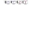
Figure 7: Effect of magnetic field gradient on the EIT resonance. (a-b) The real (a) and imaginary (b) parts of $\chi^{(D)}$ for Scheme A with a pump power 5 mW and interaction area $w_{\mathrm{int}}=2$ cm, $l_{\mathrm{int}}=0.5$ mm, and pressure $p=25$ Torr. The solid (blue online) curves show the resonance without any magnetic field gradient, while the black and gray dots are calculated with $S_{B}=2~{}$G/mm and $S_{B}=8~{}$G/mm, respectively, at the point where $B_{z}=0$. (c-d) The same calculation for Scheme B (red online).

An analytic treatment calculating the correction Eq. (18) using the non-Doppler broadened $\chi$ obtained from Eq. (13), reveals that the expected absorption at the resonance (in the absence of other decoherence mechanisms from $|4\rangle$ and $\gamma_{\mathrm{diff}}$) is $A_{\mathrm{grad}}=64(D_{g}/3)S_{B}^{2}S_{\mathrm{res}}^{2}\Gamma_{r}\gamma_{e}^{2}/|\Omega_{p}|^{6}$. We performed full numerical calculations of $\chi^{(D)}$, using Eq. (III.1), choosing values of $h_{\mathrm{int}}=0.5$ mm and $w_{\mathrm{int}}=2$ cm and a pump power 5 mW, which gives $\Omega_{p}=(2\pi)12.0$ MHz for Scheme A and $\Omega_{p}=(2\pi)16.9$ MHz for Scheme B. In Fig. 8 we show the dependence of the absorption $A$, slope $S$, and width $W$ versus $S_{B}$. The values chosen for the pressure correspond to optimal choices we discuss later. Our analytic expression above provides a reasonable estimate but is not quantitatively accurate. In particular, note the predicted quadratic dependence of the absorption $A_{\mathrm{grad}}\sim S_{B}^{2}$ holds only for very small values of $S_{B}$ then it becomes close to a linear dependence. As expected, the gradient contribution is dominant in Scheme B even for very small values of $S_{B}$, while in Scheme A the $|4\rangle$ contribution is dominant until about $S_{B}=4$ G/mm. One also notes the gradient substantially impacts the slopes $S$.

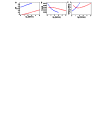
Figure 8: Dependence of EIT resonance on gradient. (a) The relative EIT absorption $R_{\mathrm{EIT}}=A/\chi^{(D)}(\Delta_{0})|_{\Omega_{p}\rightarrow 0}$ versus magnetic field gradient in Scheme A (smaller, blue dots) and Scheme B (larger, red dots). We use a pump power 5 mW and interaction area $w_{\mathrm{int}}=2$ cm, $l_{\mathrm{int}}=0.5$ mm and a pressure $p=10$ Torr for Scheme A and $p=25$ Torr Scheme B. (b) The slope $S$ of the resonance for the same parameters. (c) The width of the resonance $W$.

The performance as a delay device can be characterized again by the maximum delay with $1/e$ attenuation. For this analysis will choose the maximum optical density $D_{\mathrm{max}}=1/2A$ and then demand that the maximum detuning at the cell edges, $(S_{\mathrm{disp}}-S_{B}s_{\mathrm{res}})(0.5w_{\mathrm{int}})=\delta^{\mathrm{(max)}}=W/\sqrt{2D_{\mathrm{max}}}$ . This results in an effective slope $S_{\mathrm{eff}}=S\sqrt{2A}W/\beta_{\mathrm{eff}}$ and a delay-bandwidth product $(S_{\mathrm{eff}}D_{\mathrm{max}}/2)\beta_{\mathrm{eff}}=WS/\sqrt{2A}$, virtually identical to conventional slow light. Examination of Fig. 8 shows that the increased absorption $A$ and decreased slope $S$ in fact decrease this product with bandwidth.

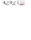
Figure 9: Dependence of EIT resonance on gradient and bandwidth. (a,b) The resulting effective susceptibility for Scheme B, with with parameters as in Fig. 7 ($S=2$ G/mm (black) and $S=8$ G/mm (gray)), when one chooses the mismatch such that $(S_{\mathrm{disp}}-S_{B}S_{\mathrm{res}})w_{\mathrm{int}}/2=\delta^{\mathrm{(max)}}$. The horizontal bars (black and gray) indicate the bandwidth $\beta_{\mathrm{eff}}$. (c) The maximum delay $\tau_{D}^{\mathrm{(max)}}=S_{\mathrm{eff}}D_{\mathrm{max}}/2$ for various gradients $S_{B}$ versus the resulting bandwidth $\beta_{\mathrm{eff}}=s_{\mathrm{res}}S_{B}w_{\mathrm{int}}$ in Scheme A (smaller, blue) and B (larger, red). We have kept the pump power 5 mW and the interaction area $w_{\mathrm{int}}=2$ cm, $h_{\mathrm{int}}=0.5$ mm constant, and chosen $p=10$ Torr for Scheme A and $p=25$ Torr for Scheme B. The inset shows a zoom in on the smaller delay points.

In Figs. 9(a-b), we show the effective dispersion curves for Scheme B the cases in Fig.7(c-d), with the mismatch chosen to be the maximum allowed difference as just described. These curves are just stretched in $\Delta_{s}$, with the stretch factor being the inverse of the ratio on the right-hand side of Eq. (20). The black and gray horizontal bars indicate the bandwidths $\beta_{\mathrm{eff}}$ (the frequencies dispersed within the $w_{\mathrm{int}}=2$ cm area) in each case. In Fig. 8(c) we plot the maximum delay versus the bandwidth in both schemes. It appears delays $\sim 5$ ns are possible over a bandwidth $\sim 50$ MHz in Scheme B, whereas similar delays are only possible over $\sim 10$ MHz in Scheme A.

To get a better sense of the sacrifices one makes to get a wider bandwidth (due to the diffusion problem) we plot in Fig. 10(a) the maximum delay-bandwidth product versus magnetic field gradient (with the same parameters as Fig. 9(c)). We see that for Scheme B we maintain full pulse separation capabilities up to bandwidths $\beta_{\mathrm{eff}}\sim 50$ MHz.

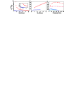
Figure 10: Dependence of delay capabilities on field gradient buffer gas pressure. (a) The maximum delay bandwidth product $\tau_{D}^{\mathrm{(max)}}\beta_{\mathrm{eff}}$ versus the slope $S_{B}$ for the same parameters as in Fig. 9(c). The inset shows a zoom in on the lower delay-bandwidth product points. Note that $S_{B}=$1 G/mm corresponds to $\beta_{\mathrm{eff}}=(2\pi)23$ MHz. (b) Same plot, but adjusting the width $w_{\mathrm{int}}$ so the bandwidth is constant, keeping the total pump power at 5 mW. The Scheme B series is chosen so that the total magnetic field difference across $w_{\mathrm{int}}$ is 40 G ($\beta_{\mathrm{eff}}=(2\pi)56$ MHz) and for the Scheme A series is 10 G ($\beta_{\mathrm{eff}}=(2\pi)14$ MHz). (c) Delay/bandwidth product versus pressure keeping $w_{\mathrm{int}}=2$ cm. The solid, large (red online) dots are Scheme B for $S_{B}=2$ G/mm and the non-solid (light red) circles are for $S_{B}=4$ G/mm. For Scheme A for $S_{B}=0.5$ G/mm (small, dark blue dots) and $S_{B}=1$ G/mm (x’s, light blue).

Because of the extremely strong dependence of $A_{\mathrm{grad}}$ with power we found numerically that one always benefits from using smaller $h_{\mathrm{int}}$, so this parameter should be chosen to be the smallest reasonable value over which the beam can be easily focused. Though too small a value $h_{\mathrm{int}}$ would lead to a higher loss from $\gamma_{\mathrm{diff}}$ this problem is almost always dominated by the diffusion in the magnetic field gradient and so is not a big consideration. Similarly, in choosing $w_{\mathrm{int}}$ we found that the gain in transparency from higher intensities tended to outweigh the gain one got from lower slopes. Figure 10(b) shows the maximum delay-bandwidth product versus $S_{B}$, but keeping the pump power constant and adjusting the interaction with $w_{\mathrm{int}}$ such that the bandwidth $\beta_{\mathrm{eff}}=(2\pi)56$ MHz was also kept constant. Indeed one sees that one gains by using steeper gradients over smaller areas. Ultimately, the slope $S_{B}$ that can be used in practice will be determined by the manner in which the magnetic field gradient and signal dispersion can be generated.

In the calculations in Figs. 9 and 10(a-b) we chose pressures $p=10$ Torr and 25 Torr for Schemes A and B, respectively. Numerically these were found to be about optimal. In Fig. 10 we plot the dependence of the of the maximum delay-bandwidth on the pressure for several cases. In Scheme A, the optimal pressures are larger than in the homogenous case due to increased importance of reducing diffusion in the magnetic field gradient. Interestingly, even in Scheme B, higher pressures eventually reduce the performance. This can be understood from the factor $\gamma_{e}^{2}$ in the analytic estimate for $A_{\mathrm{grad}}$ above. The physical origin of this factor is the fact that the EIT width $W=\Omega_{p}^{2}/\sqrt{8\gamma_{e}\Gamma_{r}}$ decreases with $\gamma_{e}$ and therefore makes the resonance more sensitive to the averaging over nearby magnetic fields Eq. (III.1). We plot the dependence on pressure for two different gradients in each scheme. While the optimal pressures are slightly different, the dependence on pressure is rather weak and so a sensitive parameter search versus $p$ should not be required.

IV Summary

We have performed a comprehensive and systematic analysis of EIT resonances, and the resulting pulse propagation characteristics, in ⁸⁷Rb vapors, including effects of couplings to additional levels in the hyperfine structure and a buffer gas. We then calculated the delays, transmissions, and bandwidths for propagation of light tuned to these resonances. We analyzed two particular $\Lambda$ level schemes (diagrammed in Fig. 1) and found that Scheme B was far superior, in terms of achievable delays and delay-bandwidth products, due to the lack of coupling to additional levels. Despite its poorer performance, Scheme A still provides reasonable performance and may be desirable since it is much easier to initialize, simply with optical pumping. Importantly, we found the EIT resonance could be shifted over a wide range of frequencies by applying a homogeneous magnetic field, and that the resonance characteristics were quite insensitive to this field over range of about 500 MHz. This analysis serves as a useful model to study EIT in conventional slow light, and also as a basis for study of our channelization architecture.

We then presented a model to analyze the effect of an inhomogenous magnetic field, which causes a strong variation of the EIT resonance frequency in the transverse direction. This was then applied to analyze the performance of our proposed channelization architecture for wide-band slow light, where a signal pulse is spatially dispersed according to frequency and an inhomogeneous magnetic field is applied in a such a way that the EIT resonance frequency matches this dispersion. We found that by choosing the magnetic field gradient so the change in the two-photon resonance is slightly mismatched from the transverse dispersion of the signal, one could achieve EIT and slow light conditions over a much larger bandwidth than with conventional slow light. This is essential for applications in many signal processing applications. We found that the diffusion of atoms in the field tended to reduce the delay-bandwidth products with bandwidth. In Scheme B, this architecture should allow a delay-bandwidth greater than unity up to bandwidths of about $\sim 50$ MHz, where delays are $\sim 5$ ns (see Fig. 8). Furthermore, we note either the pump field power or the magnetic field gradient can be used to control $S_{\mathrm{eff}}$ and thus the delay, making it a controllable time delay system.

The buffer gas is important in reducing the diffusion of atoms from into regions of widely varying magnetic field and so higher buffer gas pressures are generally desirable for higher magnetic field gradients. However, we also found that higher pressures narrow the EIT feature and can therefore increase the sensitivity of the dispersive slope and absorption profile to magnetic field gradients. Balancing these two considerations leads to an optimal pressure, which we found this optimum to be near $p\sim$10 Torr for Scheme A and $p\sim 25$ Torr for Scheme B, for reasonable parameters. This optimal pressure was not very sensitive to the exact value of the gradient and other parameters. We also found that one generally benefited from tight focusing and high magnetic gradients.

In future work, it will be useful to consider the effects of atomic diffusion at a more microscopic level. In particular, it has been found that the model used here for diffusion out of the interaction region may overestimate the loss in real systems due to the fact that atoms can diffuse back into the interaction region Irina . Additionally, dynamical jumps of velocity of individual rubidium atoms upon collisions with the buffer gas has also been found to be an important consideration bufferRot . Finally, for implementation of this system, work is also needed to develop optimal methods for transversely dispersing the signal field and producing large linear magnetic field gradients.

The role played by the differential phase shift in this system is interesting in its own right and merits further investigation. It is not entirely clear that the pulse will not be significantly more slowed than our analysis here shows, due to subtleties with the transverse dispersion of the signal. Perhaps the signal dispersion or magnetic field could be engineered in such a way that the group velocity is governed by the local (and much larger) $S$, rather than $S_{\mathrm{eff}}$, allowing much larger delays. Furthermore, it may be possible to combine this method with aspects of previous light storage experiments stoppedCold ; stoppedThermal to significantly increase the delay times.