A Quantitative Measure of Interference

Abstract

We introduce an interference measure which allows to quantify the amount of interference present in any physical process that maps an initial density matrix to a final density matrix. In particular, the interference measure enables one to monitor the amount of interference generated in each step of a quantum algorithm. We show that a Hadamard gate acting on a single qubit is a basic building block for interference generation and realizes one bit of interference, an “i-bit”. We use the interference measure to quantify interference for various examples, including Grover’s search algorithm and Shor’s factorization algorithm. We distinguish between “potentially available” and “actually used” interference, and show that for both algorithms the potentially available interference is exponentially large. However, the amount of interference actually used in Grover’s algorithm is only about 3 i-bits and asymptotically independent of the number of qubits, while Shor’s algorithm indeed uses an exponential amount of interference.

I Introduction

Entanglement and interference are believed to be key ingredients that distinguish quantum from classical information processing Bennett and DiVincenzo (2000). Indeed it has been shown that large amounts of entanglement must necessarily be generated in a quantum algorithm that offers an exponential speed-up over classical computation Jozsa and Linden (2003). Tremendous effort has been spent to develop methods to detect and quantify entanglement in a given quantum state (see Bruss (2002); De et al. for recent reviews). On the other hand very little has been done to quantify “interference”. It seems therefore well worthwhile to analyze the role of interference in quantum algorithms in more detail.

While entanglement plays an important role in many quantum information tasks, like for example quantum teleportation Bennett et al. (1993), quantum key distribution Bennett and Brassard (1984), or super–dense coding Bennett and Wiesner (1992), large amounts of entanglement may not be the only requirement to get a speed up with a quantum algorithm Jozsa and Linden (2003); Cleve et al. (1998). Classical analogues of entanglement exist Collins and Popescu (2002), for example in the context of the propagation of classical phase space density through Liouville’s equation Lakshminarayan . Even without talking about dynamics, a formal analogy of pure state quantum entanglement can be easily defined in the classical domain, if we replace wave functions in the definition of quantum entanglement by probability distributions. Arbitrary large amounts of “classical entanglement” of many-particle probability distributions (corresponding to classical correlations) can thus be created by a classical stochastic computer. However, only linear combinations of probability distributions with real positive coefficients are allowed, and this makes it impossible to efficiently realize Fourier-transforms with high contrast, a decisive ingredient in many quantum algorithms (see e.g. Shor (1994); Abrams and Lloyd (1999); Georgeot and Shepelyansky (2001)). In general it seems that interference between many computational paths plays an important role in quantum computation. It is unclear, however, how much interference, if any, is needed for a given quantum speed-up.

As a first step in the direction of answering this question, we introduce here a general interference measure that applies to any physical process which maps an initial density matrix to a final density matrix. It can be used in particular for any quantum algorithm, measurement processes, or classical communication. We use the interference measure to quantify interference in various steps of the well–known quantum algorithms of Shor Shor (1994) and Grover Grover (1997) as well as other physical examples, including photons passing through a beam-splitter or through a Mach-Zehnder interferometer, decoherence through bit-flip and phase errors, and quantum teleportation.

II The Essence of Interference

The familiar example of a double slit experiment, where waves with different wave-vectors are superimposed at the slits, propagate and interfere to generate an interference pattern, i.e. a certain probability distribution on the screen in a position basis, contains the basics of any interference experiment:

1. Interference needs coherence. An interference measure has to distinguish between coherent and incoherent propagation. This means first of all that interference is a property of a propagator of states, not of a state itself, in contrast to entanglement.

2. Coherent propagation alone does not amount to interference, however. For example a quantum gate which implements just the unitary identity operation is completely coherent (a pure state remains a pure state), whereas there is no interference at all: the probability for each final basis state depends only on the initial amplitude of the same basis state. Similarly, there is no interference for a quantum gate that just permutes in-coming amplitudes. Evidently, at least two states have to be coherently superposed. Generally speaking, the amount of interference should be linked to how many different initial state amplitudes contribute to each final state amplitude, and to what extent. An interference measure should be maximized if each basis state as input state produces an “equipartitioned” output state, i.e. a state with the same absolute probability amplitude for each basis state.

3. Interference is basis dependent. Indeed, no interference pattern at all, but a probability distribution just reflecting the initial amplitudes would be observed in the double slit experiment described above, if the output were observed in the momentum basis. Also any unitary evolution is given by a unitary matrix $U$ defined in a specific basis (for example the computational basis for a quantum algorithm). This matrix can always be diagonalized, and in the new basis the propagator then just corresponds to a multiplication with a phase factor for each input basis state, which does clearly not amount to interference.

III The interference measure

III.1 General formulation

We start by defining a measure of coherence for a general propagator $P$ of a density matrix, $\rho^{\prime}=P\rho$, where $P$ is a super-operator specified in the computational basis, such that, written in components,

$$\rho_{ij}^{\prime}=\sum_{k,l}P_{ij,kl}\rho_{kl}\,.$$ (1)

Further below we will adapt this formalism to the “operator sum formalism” more familiar in the context of quantum computation Nielsen and Chuang (2000).

Consider a black box which maps an initial density matrix to a final probability distribution, as is normally the case for a quantum computer if the read-out process is considered part of the algorithm. As long as one regards a unique input state (pure or mixed), one cannot distinguish between coherent and incoherent propagation. Indeed, the black box might forget about any initial phase information, keep just the initial probabilities and then use a stochastic matrix which maps them to the probability distribution of the desired final state. The final probabilities are then invariant under arbitrary phase rotations of the initial amplitudes. To distinguish between coherent and incoherent propagation, an interference measure must therefore quantify the dependence of the final probabilities on the initial phases — a strategy which is in fact often employed experimentally to show coherence.

Let us therefore start with a pure initial state, $\rho=|\psi\rangle\langle\psi|$, with $|\psi\rangle=\sum_{j=1}^{N}a_{j}|j\rangle$. The amplitudes $a_{j}$ with phases $\varphi_{j}$, $a_{j}=|a_{j}|{\rm e}^{{\rm i}\varphi_{j}}$, lead to final probabilities

$$p_{i}^{\prime}=|\rho_{ii}^{\prime}| = \sum_{j,k}P_{ii,jk}{\rm e}^{{\rm i}(\varphi_{j}-\varphi_{k})}|a_{j}a_{k}|\,.$$ (2)

The dependence of each individual probability on the initial phases is thus given by

$$\frac{\partial p_{i}^{\prime}}{\partial\varphi_{l}} = {\rm i}\sum_{k}|a_{k}a_{l}|\left(P_{ii,lk}{\rm e}^{{\rm i}(\varphi_{l}-\varphi_{k})}-c.c.\right)\,.$$ (3)

We define the real phase sensitivity matrix $S$ with matrix elements $S_{il}=\partial p_{i}^{\prime}/\partial\varphi_{l}$, and the positive semi–definite matrix $SS^{T}$, with $SS^{T}=0$ iff $\partial p_{i}^{\prime}/\partial\varphi_{l}=0$ for all $i,l=1,\ldots,N$. A coherence measure ${\cal C}(P)$ can be obtained by taking the trace of $SS^{T}$ and averaging it over all initial phases,

$${\cal C}(P) = \frac{1}{(2\pi)^{N}}\int_{0}^{2\pi}d\varphi_{1}\ldots d\varphi_{N}{\rm tr}(SS^{T})$$

$$= \sum_{i,k,l,m}|a_{k}a_{l}^{2}a_{m}|\left[-\int_{0}^{2\pi}\frac{d\varphi_{k}d\varphi_{l}d\varphi_{m}}{(2\pi)^{3}}P_{ii,lk}P_{ii,lm}{\rm e}^{{\rm i}(2\varphi_{l}-\varphi_{k}-\varphi_{m})}+\int_{0}^{2\pi}\frac{d\varphi_{k}d\varphi_{m}}{(2\pi)^{2}}P_{ii,lk}P_{ii,ml}{\rm e}^{{\rm i}(\varphi_{m}-\varphi_{k})}\right]+c.c$$

$$= 2\sum_{i,k}\sum_{l\neq k}|P_{ii,lk}a_{k}a_{l}|^{2}\,.$$ (5)

This measure still depends on the amplitudes of the initial state. However, coherence should be measured for an input state with amplitudes on all basis states. We therefore chose a “democratic” input state with $|a_{i}|=1/\sqrt{N}$ for all $i=1,\ldots,N$. We multiply with an additional prefactor $N^{2}/2$ and define the coherence measure

$${\cal I}(P)=\sum_{i,k,l}|P_{ii,kl}|^{2}-\sum_{i,k}|P_{ii,kk}|^{2}\,.$$ (6)

The quantity ${\cal I}(P)$ obviously has the desired property to be zero in the case of a classical stochastic propagation, that is for $P_{ij,kl}=M_{ik}\delta_{ij}\delta_{kl}$, where $M_{ik}$ is a stochastic matrix which propagates classical probabilities from initial values $p_{k}$ to final values $p_{i}^{\prime}$, $p_{i}^{\prime}=\sum_{k}M_{ik}p_{k}$, and $\delta_{ik}$ denotes the Kronecker–delta. From the definition it is clear that ${\cal I}(P)$ is non–negative. In the case where all eigenvalues of $P$ are smaller than one, as for example for dissipative quantum maps an upper bound is given by ${\cal I}(P)\leq N^{2}$, as can be seen by using the inequality $||P\psi||\leq||\psi||$ with $\psi_{kl}=\delta_{k,k_{0}}\delta_{l,l_{0}}$ for all $1\leq k_{0},l_{0}\leq N$. This bound is probably not optimal, and, as will be seen, can be improved in the case of unitary propagation.

The propagation of mixed states is in quantum information theory generally formulated within the operator sum formalism Nielsen and Chuang (2000): A set of operators $\{E_{l}\}$ acts on $\rho$ according to $\rho^{\prime}=\sum_{l}E_{l}\rho E^{\dagger}_{l}=P\rho$. The $E_{l}$’s are known as Kraus operators Kraus (1983) and obey $\sum_{k}E_{k}^{\dagger}E_{k}={\bf 1}$ for trace–preserving operations. The connection to the propagator $P$ is given by $P_{ij,km}=\sum_{l}(E_{l})_{ik}(E_{l}^{*})_{jm}$, and we can reformulate the interference measure (6) as

$${\cal I}=\sum_{i,k,m}\left|\sum_{l}(E_{l})_{ik}(E_{l}^{*})_{im}\right|^{2}-\sum_{i,k}\left(\sum_{l}\left|(E_{l})_{ik}\right|^{2}\right)^{2}\,.$$ (7)

We will now show that ${\cal I}(P)$ is in fact a good measure of interference, as it also measures the amount of equipartition in the case of unitary propagation.

III.2 Unitary propagation

Coherence is, by definition, perfect, if all pure incoming states remain pure during propagation, i.e. also the final state can be written as $\rho^{\prime}=|\Phi\rangle\langle\Phi|$, with a state $|\Phi\rangle$ related to $|\psi\rangle$ by a unitary transformation, $|\Phi\rangle=U|\psi\rangle$. In this case $P$, which we shall denote by $P(U)$, has matrix elements $P_{ii,kl}=U_{ik}U^{*}_{il}$. Profiting further from the fact that $\sum_{i,k,l=1}^{N}|U_{il}U_{ik}|^{2}=N$ due to the unitarity of $U$, we find in this case

$${\cal I}(P(U)) = \left(N-\sum_{i,k}|U_{ik}|^{4}\right)\,.$$ (8)

In the unitary case the coherence measure (8) has the property that $0\leq{\cal I}(P(U))\leq N-1$. The right hand side of this inequality is easily verified using the Cauchy–Schwarz inequality applied to all vectors $(|U_{i1}|^{2},\ldots,|U_{iN}|^{2})$ ($i=1,\ldots,N$), and $(1/\sqrt{N},\ldots,1/\sqrt{N})$, and is in fact the optimal bound, as it is reached for $|U_{ik}|=1/\sqrt{N}$ for all $i,k$. The left hand side follows from the positivity of $SS^{T}$, or explicitly from $\sum_{i,k}|U_{ik}|^{4}\leq\sum_{i,k}|U_{ik}|^{2}=\sum_{k}1=N$, where we have used that $0\leq|U_{ik}|^{2}\leq 1$ due to $\sum_{i}|U_{ik}|^{2}=1$.

The term $\sum_{ik}|U_{ik}|^{4}$ is nothing but the inverse participation ratio (IPR) of a column $k$ of the unitary matrix summed over all columns. The IPR is a well–known measure of “equipartition” of a wave-function, used extensively in solid state physics in order to measure localization Wegner (1980). A column of $U$ with an amplitude on a single basis state, i.e. $U_{ik}=\delta_{ii_{k}}$ for column $k$ and some index $i_{k}$ gives $\sum_{i}|U_{ik}|^{4}=1$. If all columns have an entry on just a single basis state we get therefore $\sum_{ik}|U_{ik}|^{4}=N$.

Thus, if $U_{ik}=\delta_{iP_{i}(k)}$, where $P_{i}(k)$ is a permutation, we have ${\cal I}(P(U))=0$. This reflects just the fact that this kind of coherence is useless — the final probability distribution does not depend at all on the initial phases and for all possible input states, the same output could be obtained with a propagation of probabilities only.

On the other hand, perfectly “equipartitioned” output states for each computational basis state used as input, $|U_{ik}|=1/\sqrt{N}$ for all $i,k$, give $\sum_{ik}|U_{ik}|^{4}=1$. Therefore, ${\cal I}$ measures for unitary propagation also the amount of equipartition, where ${\cal I}(P(U))$ varies between 0 for a mere permutation of all input states and $N-1$ if all output states corresponding to computational basis input states are perfectly equipartitioned. We therefore define ${\cal I}(P)$ in eq.(6) as the measure of interference in the propagator $P$. Note that this definition is very general, and might be applied to any physical situation where (possibly mixed) input states are propagated to (possibly mixed) output states.

III.3 Properties of the interference measure

III.3.1 Invariances

As eq.(6) contains a double and triple sum over all computational basis states, it is obvious that ${\cal I}$ is invariant under a permutation of the computational basis states. This goes hand in hand with the observation that a pure permutation of the computational basis states does not generate any interference. It is also obvious that ${\cal I}$ is invariant under arbitrary phase changes of any matrix element $P_{ij,kl}$. For unitary propagation, the inverse propagation $U^{\dagger}$ leads to the same amount of interference, ${\cal I}(P(U^{\dagger}))={\cal I}(P(U))$.

III.3.2 Equipartition in a Sub-Space

Consider a unitary matrix with $|U_{ik}|=1/\sqrt{M}$ for $1\leq i,k\leq M$ for some integer $M\leq N$, and $|U_{ik}|=\delta_{ik}$ for $i>M$ or $k>M$. Straightforward evaluation of ${\cal I}(P(U))$ from eq.(8) gives ${\cal I}(P(U))=M-1$. Thus, ${\cal I}(P(U))$ increases indeed linearly with the number of coherently superposed states.

III.3.3 Adding auxiliary qubits

Another situation, encountered often in quantum computing, is the addition of auxiliary qubits, or in general a Hilbert space of dimension $M$ connected by a tensor product to the original Hilbert space. As long as one acts on the auxiliary qubits only with the identity operation, their only effect is to increase the number of coherently superposed states by a factor $M$. One should therefore expect the amount of interference of $\tilde{U}=U\otimes{\bf 1}_{M}$ to be larger by a factor $M$ compared to ${\cal I}(P(U))$. This is indeed the case. To see this, define the matrix elements of $\tilde{U}$ as $\tilde{U}_{nmkl}=U_{nk}{\bf 1}_{ml}=U_{nk}\delta_{ml}$. Then we have from eq.(8), ${\cal I}(P(\tilde{U}))=NM-\sum_{n,m,k,l}|U_{nk}|^{4}\delta_{ml}=M(N-\sum_{n,k}|U_{nk}|^{4})=M{\cal I}(P(U))$. The corresponding calculation can be done for the general non–unitary propagation of a density matrix $\rho=\rho^{A}\otimes\rho^{B}$, such that $\rho^{\prime}=\tilde{P}\rho=(P\rho^{A})\otimes\rho^{B}$, and the result is the same: ${\cal I}(\tilde{P})=M{\cal I}(P)$.

III.3.4 The “i-bit” and the Hadamard gate

The linear dependence of the interference measure on the number of coherently superposed states makes it possible to define a unit of interference. We can define the number $n_{I}$ of “interference bits” (or “i-bits” for short) that measures the (logarithmic) amount of interference in a propagator $P$ as

$$n_{I}=\log_{2}({\cal I}(P)+1)\,.$$ (9)

As an immediate consequence we find that a Hadamard gate, $H_{ij}=(-1)^{ij}/\sqrt{2}$ for $i,j\in{0,1}$, generates one bit of interference as ${\cal I}(P(H))=1$, and this is the maximum possible amount of interference for the unitary propagation of a single qubit. Moreover, it is easy to show that for a tensor product of $n$ Hadamard gates acting in parallel on $n$ qubits, also called the Walsh–Hadamard transform, $W=H\otimes H\otimes\ldots\otimes H$, one obtains $n$ i-bits, ${\cal I}(P(W))=2^{n}-1$, as the amplitude of each matrix element of the tensor product has an absolute value $1/2^{n/2}$. One may thus consider the Hadamard gate as a “currency” of interference in a quantum algorithm, much as a singlet measures the amount of entanglement in a bipartite quantum state. Note, however, that not each Hadamard gate in a quantum algorithm adds an i-bit to the total amount of interference. If $p$ Hadamard gates act on $p$ different qubits out of a total number of $n$ qubits, the interference is ${\cal I}=2^{n}-2^{n-p}$.

III.4 Potentially available interference versus actually used interference

Another reason why a Hadamard gate does not necessarily add an i-bit of interference to a quantum algorithm lies in the fact that the amount of interference added in a given step of the algorithm depends on the transformation built in all previous steps. This is easily seen from the example of two Hadamard gates in series, acting on a single qubit, $H^{2}={\bf I}_{2}$, such that ${\cal I}(P(H^{2}))=0$. We will call “accumulated interference” the total interference ${\cal I}(P_{m}\ldots P_{1})$ of a sequence of transformations $P_{m}\ldots P_{1}$, which is in general very different from the sum of interferences of each step $P_{i}$. In principle one can calculate the accumulated interference for an arbitrary part of any quantum algorithm, but most interesting is in general the accumulated interference of the entire algorithm.

It turns out that many quantum algorithms generate a lot of interference right at the beginning, including Shor’s and Grover’s algorithms (see below), as they start out with the Walsh–Hadamard transform on many qubits. In the end the desired information (e.g. the period of a function or the label of a searched state) has to be extracted, which is done by a reduction of the accumulated interference, as the probability distribution gets concentrated on only very few computational states. The Fourier transform, which taken by itself would add even more interference, performs this task in Shor’s algorithm.

However, not all quantum algorithms actually use all the interference generated. A tremendous “waste” of interference can arise when only a single column of the unitary matrix corresponding to a single initial state (e.g.  $|0\ldots 0\rangle$) is used, whereas it is completely irrelevant what happens in the other columns. One might be tempted to calculate the interference just corresponding to that initial state. Formally this can be done by including a projection onto the state $|0\ldots 0\rangle$ in the algorithm, but it is easily shown that then the accumulated interference of this projection combined with whatever unitary operation follows vanishes. All coherence is destroyed in the sense that the final probability distribution is independent of the single remaining initial phase. An alternative approach is to calculate the accumulated interference for the remaining algorithm $\tilde{U}$ after the initial Walsh–Hadamard transform, i.e. once amplitudes from all computational states are available in the superposition. This amounts to changing the initial state. Then all columns of $\tilde{U}$ do contribute, and as a consequence ${\cal I}(P(\tilde{U}))$ is a more realistic measure of the interference actually used. The interference measures corresponding to $U$ and $\tilde{U}$ therefore give complementary information (total “potentially available” interference in the algorithm and “actually used” interference, respectively) and will be calculated below for Grover’s and Shor’s algorithms.

IV Applications

IV.1 Beam splitter

A beam splitter transforms two photon modes with annihilation (creation) operators $a,b$ ($a^{\dagger},b^{\dagger}$), respectively, according to the unitary transformation $U_{\rm BS}=\exp(\theta(a^{\dagger}b-ab^{\dagger}))$ Nielsen and Chuang (2000). The action of $U_{\rm BS}$ on a state $|nm\rangle$ with $m$ photons in mode $a$ and $n$ photons in mode $b$ can be easily derived with the help of the relations $U_{\rm BS}aU_{\rm BS}^{\dagger}=a\cos\theta+b\sin\theta$ and $U_{\rm BS}bU_{\rm BS}^{\dagger}=b\cos\theta-a\sin\theta$. We exploit the fact that the total number $N$ of photons in the two modes is conserved to write the matrix elements of $U_{\rm BS}$ as

$$(U_{\rm BS}^{(N)})_{im} \equiv \langle i\,\,N-i|U_{\rm BS}|m\,\,N-m\rangle$$ (10)

$$= \sqrt{\frac{i!(N-i)!}{m!(N-m)!}}\sum_{l={\rm Max}(m-i,0)}^{{\rm Min}(N-i,m)}{m\choose l}{N-m\choose N-i-l}(-1)^{l}(\cos\theta)^{m+N-i-2l}(\sin\theta)^{i-m+2l}\,.$$

For example, the dual-rail representation Nielsen and Chuang (2000) with logical states $|01\rangle$ and $|10\rangle$ leads to the $2\times 2$ rotation matrix

$$U_{\rm BS}^{(1)}=\left(\begin{array}[]{cc}\cos\theta&-\sin\theta\\ \sin\theta&\cos\theta\end{array}\right)\,,$$ (11)

with the amount of interference ${\cal I}(P(U_{\rm BS}^{(1)}))=2(1-\cos^{4}\theta-\sin^{4}\theta)$. Thus a maximum interference of 1 i-bit can be achieved for $\theta=\pi/4$, in which case the beam splitter realizes indeed just a Hadamard gate, up to phase shifts. The function ${\cal I}(P(U_{\rm BS}^{(N)}(\theta)))$ appears to be periodic with period $\pi/2$ for all $N$. The maximum amount of interference increases approximatively linearly with $N$ and is reached for sufficiently large $N$ at $\theta=\pi/4$. With increasing $N$, the maximum is reached more and more rapidly as function of $\theta$, and ${\cal I}$ remains almost flat in a broader and broader interval around the maximum (see figure 1).

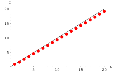
Figure 1: (Color online) Amount of interference ${\cal I}$ generated by a beam splitter as function of the angle $\theta$ and $N=1,\ldots 20$ photons (top). The amount of entanglement at $\theta=\pi/4$ increases approximately linearly with $N$ (bottom). The full line is ${\cal I}=N$.

IV.2 Mach-Zehnder interferometer

A Mach-Zehnder interferometer consists of two beam splitters in series, with an additional phase shifter in one of the two arms Nielsen and Chuang (2000). The second beam splitter is inverted relative to the first one, such that the total unitary propagation for $N$ photons is given by

$$U_{\rm MZ}^{(N)}=U_{\rm BS}^{(N)}U_{\rm P}U_{\rm BS}^{(N)\dagger}\,.$$ (12)

The phase shifter acts on a $m$ photon state in mode $a$ as $U_{\rm P}|nm\rangle={\rm e}^{{\rm i}\phi m}|nm\rangle$. The interference generated by the Mach-Zehnder interferometer is periodic in $\theta$ and $\phi$ with periods $\pi/2$ and $2\pi$, respectively (Figure 2). Again, ${\cal I}(P(U_{\rm MZ}^{(N)}))$ becomes more and more flat around the maximum with increasing $N$. The settings $\theta=\pi/2$, or $\theta=\pi/4$ or $3\pi/4$ and $\phi=\pi$, lead to a minimum of ${\cal I}$ in the range of $N$ investigated ($N=1,\ldots,20$). Finally, $\phi=0$ never leads to any interference, as in this case the interferometer just performs the identity operation.

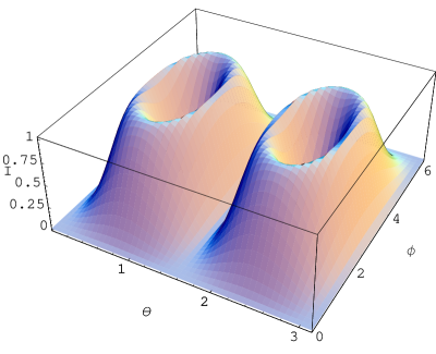
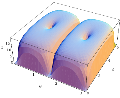
Figure 2: (Color online) Accumulated interference generated in a Mach-Zehnder interferometer as function of the angles $\theta$ and $\phi$ for 1 photon (top) and 20 photons (bottom). Note the different scale.

IV.3 Decoherence: bit flip errors and phase errors

The error operators for a bit flip error in a single qubit are given by $E_{0}=\sqrt{p}{\bf 1}_{2}$, $E_{1}=\sqrt{1-p}X$, where $X$ is the Pauli $\sigma_{x}$ matrix and $p$ the probability for no error to occur. Similarly, the error operators for a phase error in a single qubit read $F_{0}=\sqrt{p}{\bf 1}_{2}$, $F_{1}=\sqrt{1-p}Z$, where $Z$ is the Pauli $\sigma_{Z}$ matrix. One easily shows using eq.(7) that the amount of interference vanishes for both types of errors, as it should of course be, due to the fact that these are purely decohering processes. More interesting is the situation where we first apply a Hadamard gate and then the errors. That is, the Kraus operators are now ${E_{0}H,E_{1}H}$ for a bit flip error after the Hadamard gate, and ${F_{0}H,F_{1}H}$ for a phase error after the Hadamard gate. In the first case, we obtain ${\cal I}=(1-2p)^{2}$. As it should be, the interference is completely conserved, ${\cal I}=1$, for $p=0$ or $p=1$, i.e. when bit flips either never occur or do occur with certainty. Even in the latter case the interference is perfect, as the bit flip just corresponds to a unitary permutation. On the other hand, in the case of a phase flip after a Hadamard gate, interference is always conserved, i.e. ${\cal I}=1$ independent of $p$. While this might be surprising at first, it is in fact a remarkable property of ${\cal I}$ to detect that the phase error does not modify at all an interference pattern obtained by coherently superposing $|0\rangle$ and $|1\rangle$. To see this, we start with the initial state $({\rm e}^{{\rm i}\varphi}|0\rangle+|1\rangle)/\sqrt{2}$. After the Hadamard gate this state becomes $({\rm e}^{{\rm i}\varphi}(|0\rangle+|1\rangle)+(|0\rangle-|1\rangle)/2$. With probability $p$ the state remains the same, while with probability $1-p$ a phase error flips the sign in front of the $|1\rangle$ states. One obtains thus the final density matrix $\rho_{f}=\cos^{2}(\varphi/2)|0\rangle\langle 0|+\sin^{2}(\varphi/2)|1\rangle\langle 1|+(1/2-p){\rm i}\sin\varphi(|1\rangle\langle 0|-|0\rangle\langle 1|)$. Clearly, the probabilities to find 0 or 1 in the final state are unaffected by the phase error, and one gets a perfect interference picture for any value of $p$, as the phase errors from the bra and the ket cancel. Note that by just looking at the off-diagonal matrix elements of $\rho_{f}$ (as is often done to estimate the amount of coherence in a state) one concludes that complete decoherence and the reduction to a classical mixture occurs at $p=1/2$, whereas for $p=0$ or $p=1$ a completely coherent final state is retained. This is, however, irrelevant for the success of the interference experiment, and correctly detected by our interference measure.

More generally, one might consider the action of the phase error as a measurement of the interference pattern. Indeed, $Z$ is diagonal in the computational basis, which thus constitutes the “pointer basis” of $Z$ Zurek (1981). The measurement reveals the interference pattern, but does not destroy it. It is therefore reasonable to demand that an interference measure be conserved during the measurement process. The fact that interference can be conserved during measurements is crucial also for quantum teleportation.

If a phase error occurs after the phase shifter in the Mach-Zehnder interferometer, the interference is reduced. For the example of one photon the Kraus operators are given by $G_{0}=\sqrt{p}U_{\rm BS}^{(1)}U_{\rm P}U_{\rm BS}^{(1)\dagger}$ and $G_{1}=\sqrt{1-p}U_{\rm BS}^{(1)}ZU_{\rm P}U_{\rm BS}^{(1)\dagger}$. The general expression for the interference is somewhat cumbersome, but simplifies for beam splitters with $\theta=\pi/4$ to ${\cal I}=(\sin\varphi(1-2p))^{2}$. So the interference in the Mach-Zehnder interferometer is clearly completely destroyed for $p=1/2$, as is to be expected.

IV.4 Quantum Teleportation

Alice can teleport an unknown quantum state of a qubit 1 to Bob, by doing the following Bennett et al. (1993): She first prepares two auxiliary qubits (2,3) in the Bell state $(|00\rangle+|11\rangle)/\sqrt{2}$, and sends qubit 3 to Bob. We will consider the Bell state preparation as part of the protocol, as it will become clear that already here a certain amount of interference is used . Starting from state $|00\rangle$ of qubits (2,3), Alice can prepare the Bell state by applying $H$ to qubit 3 ($H_{3}$, step 1) and then a CNOT with 3 as control and 2 as target ($C_{32}$) to qubits (2,3) (step 2). Next Alice applies a CNOT with 1 as control and 2 as target ($C_{12}$) to qubits (1,2) (step 3) and a Hadamard to qubit 1 ($H_{1}$, step 4). She then measures qubits (1,2) in the computational basis (step 5), and sends the result ${m_{1},m_{2}}$ (where $m_{i}=$ 0 or 1) to Bob through a classical channel. Bob performs the unitary operation $Z^{m_{1}}X^{m_{2}}$ (step 6). The total propagation of the density matrix thus reads

$$\rho^{\prime}=\sum_{i,j=0,1}Z^{j}X^{i}E_{ij}H_{1}C_{12}C_{32}H_{3}\rho\left(Z^{j}X^{i}E_{ij}H_{1}C_{12}C_{32}H_{3}\right)^{\dagger}\,,$$ (13)

where the $E_{ij}$ are projectors, $E_{ij}={\bf 1}\otimes|ij\rangle\langle ij|$, and the qubits are numbered from right to left.

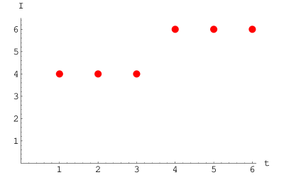
Figure 3: (Color online) Accumulated interference during the quantum teleportation protocol Bennett et al. (1993). On the t-axis is the step number (see text). The interference is plotted for the entire propagator up to and including step number $t$. Interference only arises during the application of the two Hadamard gates and is conserved during all other steps, including the measurement (step 5). A maximum amount of interference of about 2.58 i-bits (${\cal I}=6$) is generated.

Figure 3 shows how the amount of interference used in this protocol evolves step by step. Obviously already the creation of the initial entangled state uses interference, through the application of the Hadamard gate in qubit 3 (step 1). Qubits 1 and 2 are left alone, therefore the total amount of interference is ${\cal I}(P(H\otimes{\bf 1}_{4}))=4$. In fact, interference is only generated by Hadamard gates in this algorithm, and the largest amount of interference reached is ${\cal I}=6$, or almost three i-bits. Remarkably, the interference is not destroyed in the measurement process.

IV.5 Shor’s algorithm

Shor’s algorithm Shor (1994) enables one to factor a large integer number $R$ into primes using a polynomial number of operations. The initial state is prepared in two registers of size $2L$ and $L$, where $L=[\log_{2}R]+1$ ($[.]$ denotes the integer value), with a total number of qubits $n=3L$. The algorithm can be decomposed into three parts. First, the state $|0\ldots 0\rangle|0\ldots 01\rangle$ is transformed into $N^{-1/2}\sum_{t=0}^{N-1}|x\rangle|1\rangle$ (where $N=2^{2L}$ equals the dimension of the Hilbert space of $2L$ qubits) by the use of $2L$ Hadamard gates applied to each qubit separately. As mentioned in section III.3.4, this part generates the amount of interference, ${\cal I}=2^{n}-2^{L}$. This value of ${\cal I}$ corresponds to the maximum value of ${\cal I}$ for transformations of the first register alone. On the other hand, no entanglement is created since the state remains factorizable. In a second part, the state is transformed in $O(n^{3})$ operations into $N^{-1/2}\sum_{t=0}^{N-1}|x\rangle|f(x)\rangle$ where $f(x)=a^{x}\;(\mbox{mod}\;R)\;$. This part can be viewed as a permutation matrix: each line and each column has only one nonzero entry. Therefore the interference measure for this transformation alone gives zero. On the other hand, it creates entanglement. The third part consists of a Quantum Fourier Transform (QFT) on the first register only which allows one to find the period of the function $f$. The corresponding operator on the first register can be written as a matrix whose entries are all of absolute value $1/\sqrt{N}$. As such, the QFT alone maximizes the interference measure (6) on the first register, corresponding to ${\cal I}=2^{n}-2^{L}$ , in the same way as the Walsh-Hadamard transform. In contrast with the latter, the QFT contains two-qubit gates and creates some entanglement. We note that nevertheless numerical simulations for small number of qubits seem to indicate that most of the entanglement is created during the second phase where no interference is built up or used Kendon and Munro .

It is interesting to note that various versions of the factorization algorithm have been proposed which aim at minimizing the number of gates and/or qubits Zalka ; Beauregard (2003). They often use quantum Fourier transforms to gain efficiency in the process $N^{-1/2}\sum_{t=0}^{N-1}|x\rangle|0\ldots 01\rangle$ $\rightarrow N^{-1/2}\sum_{t=0}^{N-1}|x\rangle|f(x)\rangle$, for example using instances of the Schönhage-Strassen algorithm which is more efficient than usual multiplication for very large numbers. Thus these methods generate some interference in the second part of the algorithm, where usually only entanglement is produced. In some sense, this “acceleration” of the factorization algorithm is made by trading interference and entanglement.

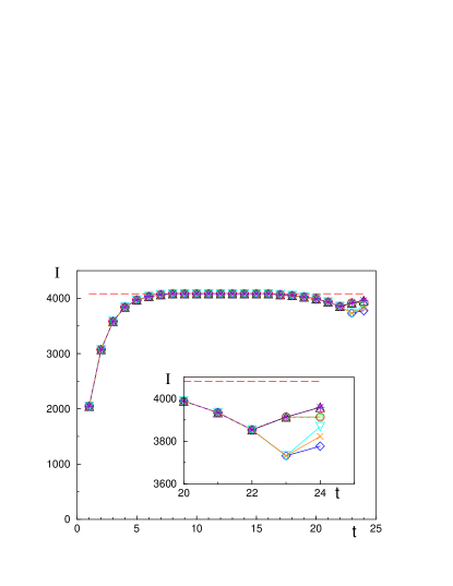
Figure 4: (Color online) Accumulated interference generated during Shor’s algorithm for factorization of $R=15$ ($L=[\log_{2}R]+1=4$ and in total $n=3L=12$ qubits). On the t-axis is the step number (see text). The interference is plotted for the entire propagator up to and including step number $t$. Values of $a$ are $a=13$ (circles, full red line), $a=7$ (squares, dashed green line), $a=11$ (diamonds, full blue line), $a=8$ (triangles up, full black line), $a=14$ (triangles down, full cyan line), $a=4$ (crosses, full orange line), $a=2$ (stars, dashed violet line). Data for different values of $a$ differ only for the last two time steps. Data from $a=13$ and $a=7$ are the same, as are data from $a=8$ and $a=2$. The horizontal dashed red line is the maximum possible value of interference for an untouched second register, ${\cal I}=2^{n}-2^{L}=4080$. The inset shows the same curves for the last steps on a different scale. Lines are there to guide the eye only. Massive interference ${\cal I}=2^{n}-2^{L}$ (or almost $n$ i-bits) is generated during the application of the Walsh-Hadamard gate (part 1, first eight points). Interference is unchanged in part 2 (next eight points), and decreases during the last part (QFT) (last eight points).

Figure 5: Accumulated interference up to and including step number $t$ generated during Shor’s algorithm, excluding the initial Walsh–Hadamard transform for factorization of $R=15$ ($n=12$ qubits). The step number on the t-axis is the same as in figure 4 but shifted by $8$. Horizontal dashed red line is maximum possible value of interference for transformations of the first register alone ${\cal I}=4080$. The accumulated interference is changed only during the final quantum Fourier transform, and does not depend on the value of $a$. The actually used interference shown here is comparable with the potentially available interference shown in figure 4.

Figure 4 shows the accumulated interference for the factorization of $R=15$. Shor’s algorithm requires $a$ to be chosen coprime to $R$. We therefore show data for the seven possible values $a=2,4,7,8,11,13,14$. The initial Walsh-Hadamard transform corresponds to the first eight value of time (the interference measure is calculated after each Hadamard gate). As explained in III.3.4, after $k$ Hadamard gates the value of ${\cal I}$ is ${\cal I}=2^{n}-2^{n-k}$. The whole transform generates an exponential amount of interference ${\cal I}=2^{n}-2^{L}=4080$, which corresponds to the maximum value possible for a transformation of the first register alone.

The next eight time values correspond to the construction of $f(x)=a^{x}\;(\mbox{mod}\;R)\;$ in the second register. Each time value corresponds to multiplication modulo $R$ of the second register by $a^{2^{i}}$, controlled by the value of the $i^{th}$ qubit of the first register. Each operation corresponds to a permutation in the computational basis, and does not affect the accumulated interference.

The last part (QFT) corresponds to the last eight time values in figure 4. Each time step corresponds to a Hadamard gate followed by controlled phase transformations, which together build the QFT. Although the QFT taken alone generates interference, its net effect is to decrease the total accumulated interference by a small amount which depends on $a$. This is actually reasonable, since this last part concentrates probability on a certain number of states which depend on the value of $a$ and $R$. It is interesting to note that the first six steps give the same values of ${\cal I}$ for all values of $a$. Only in the last two steps (corresponding to the least significant bits in the first register) does one see a branching. The first one distinguishes between the two values of the period of $f(x)=a^{x}\;(\mbox{mod}\;R)\;$ (the period is $2$ for $a=4,11,14$ and $4$ for $a=2,7,8,13$), and the last operation distinguishes further between values of $a$. Data from $a=13$ and $a=7$ are the same, as are data from $a=8$ and $a=2$, which is consistent with the fact that for these values of $a$ the set of values of $a^{x}\;(\mbox{mod}\;R)\;$ is the same. Other values of $a$ correspond to different interference even though the period of $f(x)$ may be the same since the total interference depends not only on the period of $f(x)$ but also on the period of $yf(x)$. The total interference which was exponentially large after the first two parts presumably remains so after the QFT, since for $R=15$ it goes down only by up to $7\%$. Note that it can go down and up in the last operations of the QFT.

A more realistic picture of the accumulated interference “actually used” is obtained by calculating the interference measure for the operator obtained by omitting the initial Walsh-Hadamard transform (see section III D). This corresponds to the same algorithm but with initial state $N^{-1/2}\sum_{t=0}^{N-1}|x\rangle|1\rangle$. This is shown in figure 5, where the time steps thus correspond to the last sixteen time steps in figure 4. The interference measure is zero after the first part (construction of $f(x)=a^{x}\;(\mbox{mod}\;R)\;$ in the second register), which is in accordance with the fact that all eight steps corresponding to this part can be understood as permutations. On the contrary, the interference measure grows exponentially in the last (QFT) part, and reaches the maximum value $2^{n}-2^{L}$ (for transformations of the first register only). Thus the actually used interference is clearly exponential for the factorization algorithm.

IV.6 Grover’s algorithm

Grover’s algorithm $U_{G}$ Grover (1997) can find a single marked item in an unstructured database of $N$ items in $O(\sqrt{N})$ quantum operations, to be compared with $O(N)$ operations for the classical algorithm. The algorithm starts on a system of $n$ qubits (Hilbert space of dimension $N=2^{n}$) with the Walsh-Hadamard transform $W$, thus by building an uniform superposition of the basis states $N^{-1/2}\sum_{x=0}^{N-1}|x\rangle$. Then the algorithm iterates $k$ times the same operator $U=WR_{2}WR_{1}$, with an optimal value $k=[\pi/(4\theta)]$ and $\sin^{2}\theta=1/N$ Boyer et al. (1996), i.e. $U_{G}=(WR_{2}WR_{1})^{k}W$. As mentioned in section III.3.4, $W$ generates, taken for itself, the maximum possible amount of interference ($n$ i-bits). The oracle $R_{1}$ multiplies the amplitude of the marked item (the one searched by the algorithm) with a factor $(-1)$, and keeps the other amplitudes unchanged. The corresponding $N\times N$ matrix is diagonal, making evident that its interference measure is zero. The operator $R_{2}$ multiplies the amplitude of the state $|0\ldots 0\rangle$ with a factor $(-1)$, keeping the others unchanged. By the same argument as for $R_{1}$, it generates no interference. Therefore all interference in the algorithm is generated by the Walsh-Hadamard transforms $W$. It is interesting to note that both operators $R_{1}$ and $R_{2}$ can be understood as multicontrolled gates which create entanglement, whereas $W$ cannot create entanglement as it is composed of one-qubit operations. So Grover’s algorithm alternates entanglement creation and interference creation during its evolution. We note that the interference is independent of the label of the searched item, as the interference measure ${\cal I}$ is invariant under permutation of the computational basis states.

Figure 6 shows the evolution of the accumulated interference during Grover’s algorithm in $n$ qubits. In this figure, to avoid repetition, we took the Walsh-Hadamard transform as one single time step, contrary to the preceding section. Thus step 1 corresponds to the first application of the Walsh-Hadamard transform, which generates the massive interference ${\cal I}=2^{n}-1$; step 2 is the first application of the oracle $R_{1}$, step 3 the first application of the diffusion matrix $D=WR_{2}W$, step 4 the second instance of the oracle $R_{2}$, and so on up to a total number of $2k+1$ steps. As expected, the oracle does not change the amount of interference, but the diffusion matrix reduces the accumulated interference in each step. This is crucial for the functioning of the algorithm: the probability flow is engineered in such a way that all probability gets concentrated on the computational basis state corresponding to the searched item. Therefore, the accumulated interference has to decrease, as the equipartition is decreased.

As mentioned before, most of the interference built up during the application of the $W$ gate is “wasted”, as $U$ only acts on the initial state $|0\ldots 0\rangle$. Indeed, no particular state is selected by any other column of $U$. The accumulated interference therefore reduces only very slightly, from ${\cal I}=2^{n}-1$ down to ${\cal I}\simeq 2^{n}-2$. The situation is somewhat different for Shor’s algorithm where the concentration of probability concerns many columns.

As in the case of Shor’s algorithm, it is also interesting to compute the actually used interference, i.e. the interference measure for $\tilde{U}_{G}$ obtained by omitting the initial $W$ transform, $\tilde{U}_{G}=(WR_{2}WR_{1})^{k}$ (see section III D). Figure 7 shows that this number is much smaller than the potentially available interference. Moreover, it is asymptotically independent of the number of qubits. Indeed the interference for the first application of $D$ is easily calculated analytically using the matrix elements $D_{ij}=2/N-\delta_{ij}$ in the computational basis, and gives ${\cal I}(P(D))=8-24/N+{\cal O}(1/N^{2})$. Thus, Grover’s algorithm actually uses only about three i-bits, whatever the number of qubits on which it runs! After the first application of $D$, the interference shows damped oscillations with each application of the diffusion matrix, whereas the oracle $R_{1}$ leaves the interference unchanged. Note that the oscillations would be undamped without the intermediate $R_{1}$ steps, as $(WR_{2}W)^{2}={\bf 1}$.

Thus for the Grover algorithm the maximum actually used interference after the creation of the initial equipartitioned state is small and basically independent of the number of qubits. This is in sharp contrast with the results for the Shor algorithm (preceding section) where the actually used interference grows exponentially with the number of qubits. One may speculate if this is the decisive difference that leads to exponential acceleration of Shor’s algorithm versus the $\sqrt{N}$ acceleration for Grover’s algorithm compared to the corresponding best classical algorithms known.

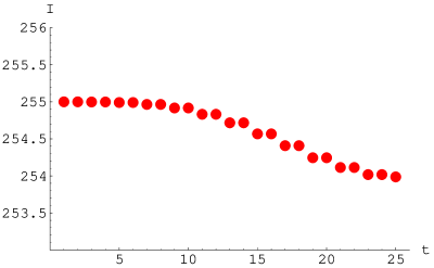
Figure 6: (Color online) Accumulated interference in Grover’s algorithm $U_{G}$ Grover (1997) for $n=8$ qubits. On the t-axis is the step number (see text). The interference is plotted for the entire propagator up to and including step number $t$. Massive maximum interference ${\cal I}_{\rm max}=2^{n}-1=255$ (or $n=8$ i-bits) is generated during the application of the Walsh-Hadamard gate (step 1) and the accumulated interference decreases subsequently during the iteration of oracle and diffusion to the value ${\cal I}\simeq 2^{n}-2$, at which point virtually all probability corresponding to the initial state $|0\ldots 0\rangle$ is concentrated on the searched state.

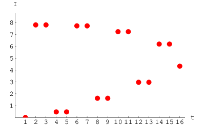
Figure 7: (Color online) Accumulated interference up to and including step number $t$ generated during Grover’s algorithm $\tilde{U}_{G}$, excluding the initial Walsh–Hadamard transform Grover (1997) for $n=7$ qubits. The step number on the t-axis is shifted by one compared to figure 6, i.e. step 1 is now the first application of the oracle $R_{1}$, which does not lead to interference. The accumulated interference is changed only during the diffusion steps $D=WR_{2}W$. The “actually used” interference shown here is much smaller than the “potentially available” interference shown in figure 6, and the maximum value ${\cal I}\simeq 8$ after the first application of $D$ is asymptotically independent of the number of qubits. This is quite different from what happens in Shor’s algorithm (compare with figure 5).

V Conclusions

We have introduced a general measure of interference, which allows to quantify interference in any physical situation which involves the propagation of a density matrix. We have defined a logarithmic unit of interference, the “i-bit” and have quantified how much interference arises in each step of the two best known quantum algorithms as well as in other physical examples, including beam splitter, Mach-Zehnder interferometer, and quantum teleportation. A beam splitter and a Mach-Zehnder interferometer generate an amount of interference proportional to the number of photons, and quantum teleportation of one qubit needs about 2.58 i-bits. Both Shor’s and Grover’s algorithm build up an exponential amount of “potentially available” interference. However, Grover’s algorithm actually uses only about three i-bits, asymptotically independent of the number of qubits on which it runs, whereas Shor’s algorithm indeed uses an exponential amount of interference. It is therefore tempting to attribute the respective exponential versus $\sqrt{N}$ acceleration of these two algorithms to the amount of interference actually used, but more work will be necessary in this direction. In particular it should be very interesting to find out if exponentially large interference is a necessary condition for an exponential speed up of a quantum algorithm compared to its classical counterpart, or if the interference measure could be used to optimize existing algorithms or to conceive new ones.