Hitting time for quantum walks on the hypercube

Abstract

Hitting times for discrete quantum walks on graphs give an average time before the walk reaches an ending condition. To be analogous to the hitting time for a classical walk, the quantum hitting time must involve repeated measurements as well as unitary evolution. We derive an expression for hitting time using superoperators, and numerically evaluate it for the discrete walk on the hypercube. The values found are compared to other analogues of hitting time suggested in earlier work. The dependence of hitting times on the type of unitary “coin” is examined, and we give an example of an initial state and coin which gives an infinite hitting time for a quantum walk. Such infinite hitting times require destructive interference, and are not observed classically. Finally, we look at distortions of the hypercube, and observe that a loss of symmetry in the hypercube increases the hitting time. Symmetry seems to play an important role in both dramatic speed-ups and slow-downs of quantum walks.

I Introduction

Algorithms based on random walks have been immensely successful in computer science. The most efficient solution for 3-SAT is based on the hitting time of a classical random walk Mot . They are also useful in algorithms for k-SAT and probability amplification. It therefore seems reasonable that their quantum analogues might be useful in developing quantum algorithms. This has been one of the main motivations for defining and analyzing quantum walks. Most quantum algorithms to date are based on the Quantum Fourier Transform (QFT), like Shor’s algorithms for factoring and discrete log Shor . But the use of QFT seems to be restricted. For example, it does not seem to be useful in some non-Abelian hidden subgroup problems like the Graph Isomorphism problem. Therefore, there is a need for new algorithmic tools for the analysis of such problems. This is another reason to study the properties of quantum walks on graphs.

Quantum walks come in two versions: continuous time and discrete time. Continuous time versions have been studied in farhi , childs , childs2 . In childs2 , it has been demonstrated that for the ”glued trees” graph, the quantum walk is exponentially faster than a classical random walk. Discrete time versions have been studied extensively for the walk on the line nayakV , bachWatrous , todd1 , todd2 and the hypercube kempe_comp , shenvi , mooreRussell . Quantum walks for any general (irregular) graphs have been defined in ambainisReview and viv . In shenvi , it was shown that there is a quadratic speed up with discrete quantum walks in searching an unstructured database for a marked node. ambainisApp describes how these concepts can be used for the problem of element distinctness. Reviews on the recent developments in this field can be found in ambainisReview and kempeReview .

Classical random walks are characterized by a number of time scales: mixing time, cover time, correlation time, and hitting time. Similar quantities can be defined for quantum walks, analogous to their classical counterparts, though some types of classical behavior are not guaranteed to hold for quantum walks. In aharanov a lower bound on the mixing time for quantum walks was found in terms of the conductance of the underlying graph. Some notions of hitting time have been defined in kempe_comp , where an upper bound on the hitting time has been found for the quantum walk on the hypercube.

In a classical discrete random walk, a hitting time is the average time for a walk beginning on a particular starting vertex to arrive for the first time at a particular ending vertex or group of vertices. It is not sufficient for the ending vertex merely to have positive probability: the particle must actually arrive there. Therefore, hitting times are generally longer than the shortest path between the starting and ending vertices. An analogous definition can be made for a continuous random walk, but in this paper we will only consider discrete walks.

This definition becomes complicated for a quantum walk, where the particle can be in a superposition of many vertex locations at once. To capture the idea of first arrival time, our definition of hitting time is the expected time for the particle to be at the final vertex for the first time as determined by a measurement of the final vertex. At every time step we perform a measurement to see if the particle is at the final vertex or not. This notion of hitting time seems to be the most natural extension of the definition of hitting time to the quantum case. Using this definition, we will obtain an expression for hitting time on any graph, and produce numerical results showing that it is orders of magnitude lower than the classical hitting time for the quantum walk on the hypercube.

This paper is organized as follows. In section II, a quantum walk on a regular graph is defined and this definition applied to a walk on the hypercube. In section III, we review the classical definition of hitting time. Then we define the quantum hitting time and derive an expression for it on any regular graph (or on an irregular graph when the walk is appropriately defined). We also briefly review other definitions of hitting time that have been used for quantum walks. In section IV, we discuss the results of simulations for a walk on the hypercube using the Grover coin, and compare them to the classical hitting time and the other definitions for a quantum hitting time, showing that in this case the hitting time is far shorter than these other definitions. Then in section V we show that the hitting time for a quantum walk can be much longer than the classical hitting time for certain combinations of initial state and coin, and can even be infinite. We demonstrate this for a walk on the hypercube with the discrete Fourier transform (DFT) coin. In section VI we look at a distorted version of the hypercube, and show that the loss of symmetry increases the hitting time. We conclude in section VII with a discussion of the role of symmetry in the speed-up of quantum walks.

II Quantum walk on the hypercube

II.1 Quantum walks

A discrete time quantum walk is defined as the application of a unitary operator $\hat{U}$ on a Hilbert space representing the graph; each vertex of the graph has a set of basis states associated with it, and the unitary operator can only cause a transition between two basis states if the vertices associated with them are connected by an edge. If the graph is regular, the Hilbert space can be a tensor product of two Hilbert spaces: in a walk on a regular graph with $N$ vertices and degree $d$, $\hat{U}$ is applied to an $Nd$-dimensional Hilbert space $\mathcal{H}^{p}\bigotimes\mathcal{H}^{c}$, where $\mathcal{H}^{p}$ is the Hilbert space of the position (i.e., the vertex), and $\mathcal{H}^{c}$ is the Hilbert space of a $d$-sided “coin,” which is “flipped” at each step to determine which edge to walk on.

For a given graph, if we label each edge incident on a vertex by a number from $1$ through $d$, such that an edge connecting two vertices gets the same label at both ends, then each vertex is a basis state in the position space and each direction is a basis state in the coin space. Therefore, the basis states for the position and coin spaces can be labelled $|0\rangle,|2\rangle,\dots,|N-1\rangle$ and $|0\rangle,|2\rangle,\dots,|d-1\rangle$. The unitary $\hat{U}$ is of the form

$$\hat{U}=\hat{S}\hat{F},$$ (1)

where we call $\hat{S}$ the shift matrix and $\hat{F}$ the coin flip matrix. $\hat{S}$ is a permutation matrix which shifts the particle from its present vertex along the edge indicated by the coin state, in a way analogous to a classical random walk. The coin flip matrix $\hat{F}$ acts solely on the coin space, so it is of the form $\hat{I}\otimes\hat{C}$. $\hat{C}$ can, in principle, be any unitary matrix, though in general we concentrate on examples with some kind of useful structure. The most common coins analyzed are the Grover coin $\hat{G}$, the Discrete Fourier Transform (DFT) coin $\hat{D}$, and the Hadamard coin $\hat{H}$. While the Grover and the DFT coins exist for all dimensions, the Hadamard coin exists only for dimensions $2^{n}$ for some $n$. These coins are given by the following matrices:

$$\hat{G}=2|\Psi\rangle\langle\Psi|-I,$$ (2)

where $|\Psi\rangle=\frac{1}{\surd{d}}\sum_{i}|i\rangle$, i.e.,

$$\hat{G}=\begin{pmatrix}\frac{2}{d}-1&\frac{2}{d}&\ldots&\frac{2}{d}\\ \frac{2}{d}&\frac{2}{d}-1&\ldots&\frac{2}{d}\\ \vdots&\ddots&\ddots&\vdots\\ \frac{2}{d}&\frac{2}{d}&\ldots&\frac{2}{d}-1\end{pmatrix},$$ (3)

$$\hat{D}=\frac{1}{\surd{d}}\begin{pmatrix}1&1&1&\ldots&1\\ 1&\omega&\omega^{2}&\ldots&\omega^{d-1}\\ \vdots&\ddots&&\ddots&\vdots\\ 1&\omega^{d-1}&\omega^{2(d-1)}&\ldots&\omega^{(d-1)(d-1)}\end{pmatrix},$$ (4)

where $\omega=\exp(2\pi i/d)$, and

$$\hat{H}_{2^{d}}=\hat{H}_{2^{d-1}}\otimes\hat{H}_{2},$$ (5)

where

$$\hat{H}_{2}=\frac{1}{\surd{2}}\begin{pmatrix}1&1\\ 1&-1\end{pmatrix}$$ (6)

The shift operator is applied after the coin operator. The shift operator moves the particle from a vertex along the edge given by the direction number of the coin state i.e.,

$$\hat{S}=\sum_{v}\sum_{i}|v(i),i\rangle\langle v,i|,$$ (7)

where $v(i)$ is the vertex connected to $v$ via the edge numbered $i$. It is interesting to note that the term ”quantum random walk” is, in a sense, a misnomer, because the randomness in a quantum walk is introduced by quantum measurements where one of the measurement outcomes takes place at random. Thus, there is no extra randomness in the walk, i.e., outside of what is introduced by quantum mechanics itself.

II.2 The Hypercube

The hypercube of dimension $n$ is a set of $2^{n}$ vertices each with a degree $n$. These vertices can be numbered by a $n$-bit string from $(00\dots 0)$ through $(11\dots 1)$. Each edge leads in a particular direction, and can be labeled by an integer $j$, $0\leq j<n$. Adjacent vertices are the ones whose bit assignments differ by a single bit. For example, for the hypercube in 3 dimensions, the vertices $(011)$ and $(111)$ are adjacent to each other, connected by an edge in the 2 direction. We can treat the bit strings of the vertices as $n$-dimensional Boolean vectors, whose elements are all 0 or 1; the directions of the edges then correspond to vectors $\vec{e}_{j}$ with element $j$ equal to 1 and all other elements zero. The vertex adjacent to a given vertex $|\vec{x}\rangle$ in the $j$ direction can be labeled $|\vec{x}\oplus\vec{e_{i}}\rangle$ $i\epsilon\{0,1,\dots,n-1\}$.

Since the vertices of the hypercube can be labeled $|0\rangle$ through $|2^{n}-1\rangle$ and the directions labeled $|0\rangle$ through $|n-1\rangle$, the Hilbert space is $\mathcal{H}^{2^{n}}\bigotimes\mathcal{H}^{n}$. The shift operator is of the form

$$\hat{S}=\sum_{j=0}^{n-1}\sum_{\vec{x}}|\vec{x}\oplus\vec{e}_{j},j\rangle\langle\vec{x},j|,$$ (8)

where $|v,j\rangle=|v\rangle\otimes|j\rangle$, $|v\rangle$ is the position state and $|j\rangle$ the coin state.

III Hitting time

III.1 Classical hitting time

Given a regular undirected graph and a particle which starts at some vertex, the classical random walk is defined as follows. At each vertex, the particle moves along any edge incident on the vertex with some predefined probability. This procedure is then repeated at the new vertex. The walk continues until the particle arrives at (“hits”) a certain vertex (called the “final vertex”) for the first time. The hitting time is defined as the average time until the particle hits the final vertex:

$$\tau(v)=\sum_{t=0}^{\infty}tp_{v}(t),$$ (9)

where $\tau(v)$ is the hitting time given that the walk starts at vertex $v$ and $p_{v}(t)$ is the probability that the particle hits the final vertex for the first time at time step $t$ (first crossing probability) given that it was at $v$ at $t=0$.

Let us now specialize to the case of the hypercube, where the the final vertex is assumed to be $11\cdots 1$. We would like to find the hitting time starting from $00\cdots 0$. For the classical walk on the hypercube, one can arrive at a recursive relation involving the hitting time. First, from the symmetry of the hypercube one can conclude that the hitting time depends only on the hamming weight of the starting vertex rather than the vertex itself. The hamming weight is the number of 1’s in the string of bits. At hamming weight $x$, there are $C^{n}_{x}=n!/x!(n-x)!$ vertices. The probability to walk to a vertex with weight $x+1$ is $(n-x)/n$, and the probability to walk to a vertex with weight $x-1$ is $x/n$. So, if $\tau(x)$ denotes the hitting time starting at any vertex with hamming weight $x$, then

$$\tau(x)=\frac{n-x}{n}\tau(x+1)+\frac{x}{n}\tau(x-1)+1,$$ (10)

with the boundary condition $\tau(n)=0$. This simplifies to

$$\Delta(x)=\frac{n-x-1}{x+1}\Delta(x+1)-\frac{n}{x+1},$$ (11)

where $\Delta(x)=\tau(x)-\tau(x+1)$. Using this recursive formula, we obtain

$$\tau(0)=\sum_{x=0}^{n-1}\Delta(x)=\sum_{x=0}^{n-1}\frac{\sum_{j=0}^{x-1}C_{x-j}^{n}+1}{C_{x}^{n-1}},$$ (12)

This sum can readily be evaluated for reasonable sizes of $n$; we use this expression to compare the classical hitting time to the quantum hitting time. We define the hitting time of a quantum walk next.

III.2 Quantum hitting time

We define the hitting time of a quantum walk in close analogy to that of a classical random walk. For a classical walk, hitting time is the average time taken for the particle to hit the final vertex for the first time. To carry this over to the quantum case, we must give a proper meaning to the phrase “for the first time.” The only reasonable way to do this is to measure the final vertex at every step to see if the particle has arrived or not. Without such a measurement at every step, one cannot appropriately define the first crossing probability. To define the hitting time this way, we first define what is called a measured quantum walk on a graph.

Suppose we have a walk on a regular graph of degree d with N vertices, where the particle begins at a vertex $x_{0}$ and walks till it reaches the vertex $x_{f}$. Assume that the coin starts in the initial state $|c_{0}\rangle$. The initial state of the particle is then,$|\Psi\rangle=|x_{0}\rangle\otimes|c_{0}\rangle$; $\rho_{0}=|\Psi\rangle\langle\Psi|$ where $\rho_{0}$ is the density operator corresponding to the initial state $|\Psi\rangle$. The measured walk is now the alternating application of a unitary evolution operator $\hat{U}$ (the product of the shift and the coin flip operators) and a projective measurement $M$ with 2 outcomes $\hat{P}_{f}$ and $\hat{Q}_{f}=\hat{I}-\hat{P}_{f}$, where $\hat{P}_{f}=|x_{f}\rangle\langle x_{f}|\otimes\hat{I}$ is the projector onto the final vertex for any coin state. Thus, if the particle is not found in the final vertex after $t$ time steps, the state is:

$$\rho_{t}=\frac{(\hat{Q}_{f}\hat{U})^{t}\rho((\hat{Q}_{f}\hat{U})^{\dagger})^{t}}{{\rm Tr}\{(\hat{Q}_{f}\hat{U})^{t}\rho((\hat{Q}_{f}\hat{U})^{\dagger})^{t}\}}.$$ (13)

If the particle is found in the final vertex, the walk is assumed to end. The state $|x_{f}\rangle$ becomes an absorbing boundary for this (measured) walk. Now, the first crossing probability at time step $t$ can be defined (analogous to the classical case) to be the following expression:

$$p(t)={\rm Tr}\{\hat{P}_{f}\hat{U}[\hat{Q}_{f}\hat{U}]^{t-1}\rho_{0}[\hat{U^{{\dagger}}}\hat{Q}_{f}]^{t-1}\hat{U^{{\dagger}}}\hat{P}_{f}\}.$$ (14)

With this definition for the probability, the hitting time becomes

$$\tau=\sum_{t=1}^{\infty}tp(t).$$ (15)

To sum this series requires a slightly different expression for the first arrival probability $p(t)$. We rewrite (14) in terms of the following superoperators (i.e., linear transformations on operators):

$$\mathcal{N}\rho=\hat{Q}_{f}\hat{U}\rho\hat{U^{{\dagger}}}\hat{Q}_{f}$$

$$\mathcal{Y}\rho=\hat{P}_{f}\hat{U}\rho\hat{U^{{\dagger}}}\hat{P}_{f}.$$ (16)

In terms of $\mathcal{N}$ and $\mathcal{Y}$, $p(t)=Tr\{\mathcal{Y}\mathcal{N}^{t-1}\rho_{0}\}$. We now evaluate the hitting time by introducing a new superoperator,

$$\mathcal{O}(l)=l\sum_{t=1}^{\infty}(l\mathcal{N})^{t-1},$$ (17)

which is a function of a parameter $l$. The hitting time now becomes

$$\tau=\frac{d}{dl}Tr\{\mathcal{Y}\mathcal{O}(l)\rho_{0}\}\biggr{|}_{l=1}.$$ (18)

If the superoperator $\mathcal{I}-l\mathcal{N}$ is invertible, then we can replace the sum (17) with the closed form

$$\mathcal{O}(l)=l(\mathcal{I}-l\mathcal{N})^{-1}.$$ (19)

If $\mathcal{I}-l\mathcal{N}$ is not invertible, then this sum instead is a pseudoinverse—that is, the inverse restricted to the support of the superoperator. So long as the graph in question is finite, this is well-defined. The derivative in (18) is then

$$\frac{d\mathcal{O}}{dt}(1)=(\mathcal{I}-\mathcal{N})^{-1}+\mathcal{N}(\mathcal{I}-\mathcal{N})^{-2}=(\mathcal{I}-\mathcal{N})^{-2}.$$ (20)

This gives us the following expression for the hitting time:

$$\tau={\rm Tr}\{\mathcal{Y}(\mathcal{I}-\mathcal{N})^{-2}\rho_{0}\}.$$ (21)

The meaning for the terms in the above expression (e.g. $\mathcal{I}-\mathcal{N})^{-2}$) can be given by vectorizing all the operators. Any matrix can be vectorized by turning its rows into columns and stacking them up one by one, so that a $D\times D$ matrix becomes a column vector of size $D^{2}$. For example:

$$\begin{pmatrix}a_{11}&a_{12}&a_{13}\\ a_{21}&a_{22}&a_{23}\\ a_{31}&a_{32}&a_{33}\end{pmatrix}\rightarrow\begin{pmatrix}a_{11}\\ a_{12}\\ a_{13}\\ a_{21}\\ a_{22}\\ a_{23}\\ a_{31}\\ a_{32}\\ a_{33}\end{pmatrix}.$$

Consequently the superoperators become matrices of size $D^{2}\times D^{2}$.

Denoting the vectorized quantities as $\rho^{v}$, etc., we obtain the hitting time as

$$\tau={\rm Tr}^{v}\{\mathcal{Y}(\mathcal{I}-\mathcal{N})^{-2}\rho^{v}\},$$ (22)

where $(\mathcal{Y}\rho)^{v}=(\mathcal{\hat{P}}_{f}\hat{U}\rho\hat{U^{{\dagger}}}\mathcal{\hat{P}}_{f})^{v}$ and $(\mathcal{N}\rho)^{v}=(\mathcal{\hat{Q}}_{f}\hat{U}\rho\hat{U^{{\dagger}}}\mathcal{\hat{Q}}_{f})^{v}$ and ${\rm Tr}^{v}\{.\}$ is the equivalent of the trace operation for vectorized quantities. It is just the inner product of the resultant vector with $I^{v}$, the vectorized identity matrix: ${\rm Tr}^{v}\{O^{v}\}=I^{v}\cdot O^{v}$.

Using Roth’s lemma roth , we obtain

$$(\mathcal{N}\rho)^{v} = \left[(\hat{Q}_{f}\hat{U})\otimes(\hat{Q}_{f}\hat{U})^{\ast}\right]\rho^{v},$$

$$(\mathcal{Y}\rho)^{v} = \left[(\hat{P}_{f}\hat{U})\otimes(\hat{P}_{f}\hat{U})^{\ast}\right]\rho^{v}.$$ (23)

Therefore, the expression for hitting time becomes

$$\tau=I^{v}\cdot\left((\hat{P}_{f}\hat{U})\otimes(\hat{P}_{f}\hat{U})^{\ast}(\mathcal{I}-(\hat{Q}_{f}\hat{U})\otimes(\hat{Q}_{f}\hat{U})^{\ast})^{-2}\rho^{v}\right).$$ (24)

III.3 Other definitions of hitting time

Two definitions of the quantum hitting time were given in kempe_comp : one-shot hitting time and concurrent hitting time. The one-shot hitting time is defined for an unmeasured walk. It is the time at which the probability of being in the final state is greater than some given value. More precisely, given some probability $p$, the one-shot hitting time is defined as the lowest time $T$ such that

$$|\langle x_{f}|\hat{U}^{T}|x_{0}\rangle|^{2}\geq p$$ (25)

where $x_{f}$ and $x_{0}$ are the final and initial states, and $\hat{U}$ is the evolution operator (as defined above). Essentially this same definition of hitting time was used in the analysis of the continuous-time walk on the hypercube in Alagic05 . This definition is useful if it is known that at some time the probability to be in the final state will be higher than some reasonable value; but for a general graph, this is not guaranteed.

The concurrent hitting time, by contrast, is defined for a measured quantum walk. Given a probability $p$, it is the the time $T$ such that the measured walk has a probability greater than $p$ of stopping at a time less than $T$. It has been proved that the concurrent hitting time is $T=\frac{\pi}{2}$ for $p=\Omega(\frac{1}{nlog^{2}n})$ for a hypercube of dimension $n$. Since we consider only the measured quantum walk in this paper, we compare our numerical results to the numerical simulation of the concurrent hitting time and the bound on it derived in kempe_comp . In the next section, this is redefined in terms of the residual probability $1-p$ and plotted against the hitting time defined in the previous section.

If we think of quantum walks as a possible route to new algorithms, then the concurrent hitting time corresponds to the time needed to find a solution with probability greater than p. The definition of hitting time used in this paper corresponds more to a typical running time for the algorithm. Both definitions could prove useful for particular purposes.

IV Numerical results

IV.1 Results for the Grover coin

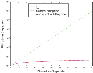
Figure 1: Hitting times of Classical and Quantum walks (semi-log scale)

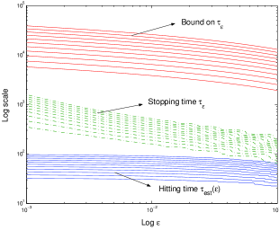
Figure 2: Comparison of Quantum hitting time, stopping time and the bound on the stopping time for dimensions 10 to 20(log scale)

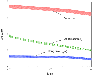
Figure 3: Comparison of Quantum hitting time, stopping time and the bound on the stopping time for dimensions 50 to 60(log scale)

We calculated the hitting time by evaluating the above expression (21) in Matlab, and comparing the result to a lower bound obtained by iterating the quantum walk for a large number of steps. Because of the multiple tensor products, the size of the matrices $\mathcal{N}$ and $\mathcal{Y}$ is $(2^{n}n)^{2}\times(2^{n}n)^{2}$.

We can make this computation more tractable in the case where the coin-flip unitary is the Grover coin $\hat{G}$ defined in (3), and the specific starting state is $\rho=|0\rangle\langle 0|\otimes|\phi\rangle\langle\phi|$, where $|\phi\rangle=\frac{1}{\surd{n}}\sum_{i=1}^{n}|i\rangle$. It was shown by Shenvi et al. shenvi that for the walk on the hypercube with this initial state and the Grover coin, the state remains always in a $2n$-dimensional subspace, where the walk is on a line with $n+1$ points. This is rather similar to the simplification made in the classical case, when we kept track only of the Hamming weight of the current vertex. With this simplification, the operators in (21) reduce to $(2n)^{2}\times(2n)^{2}$ matrices, which makes explicit calculations possible even for high dimensional hypercubes.

We write a set of basis states for this subspace as $|R,0\rangle,|L,1\rangle,|R,1\rangle,\dots,|R,n-1\rangle,|L,n\rangle$, where the first label says whether the state is “right-going” or “left-going,” and the second label gives the Hamming weight of the state. The initial state is $|R,0\rangle$, and the final state is $|L,n\rangle$. (Note that there are no states $|L,0\rangle$ or $|R,n\rangle$.) Restricted to this subspace, the $\hat{S}$ and $\hat{C}$ matrices become

$$S=\sum_{x=0}^{n}|R,x\rangle\langle L,x+1|+|L,x+1\rangle\langle R,x|$$ (26)

$$C|L,x\rangle=-cos\omega_{x}|L,x\rangle+sin\omega_{x}|R,x\rangle,$$

$$C|R,x\rangle=sin\omega_{x}|L,x\rangle+cos\omega_{x}|R,x\rangle,$$ (27)

where $\cos\omega_{x}=1-2x/n$. We see that for the walk in this subspace, the coin flip is no longer independent of the position; this is quite analogous to the reduction of the classical walk to the Hamming weight, in which the probabilities favor walking towards $x=n/2$.

Now, going back to the definition of the hitting time as a sum of series in Eq. (15) where the probability is given by Eq. (14), we can define the $\epsilon$-stopping time ($\tau_{\epsilon}$) as the time step $T$ at which the total probability $\sum_{i=1}^{T}p(i)>1-\epsilon$, where $p(i)$ is as in Eq. (14). We calculate an estimate of the hitting time ($\tau_{est}(\epsilon)$ as a function of $\epsilon$ by summing the series in Eq. (15) up to $\tau_{\epsilon}$. Figure 1 shows the classical and quantum walks on the hypercube for 100 dimensions. The exact hitting time $\tau$ calculated by computing the expression in equation (24) is plotted as the dotted line and $\tau_{est}(\epsilon)$ for $\epsilon=0.001$ is plotted as the solid line. These two lines almost coincide in the graph. The hitting time on the Y-axis is plotted in log scale. We can see that hitting time for the quantum walk is a low order polynomial whereas the classical walk is exponential. There is a very dramatic speed-up in the quantum case.

Figure 2 plots the quantum hitting time, the $\epsilon$-stopping time and the bound on the $\epsilon$-stopping time (obtained in kempe_comp ) against $\epsilon$ for dimensions from 10 to 20. Both the axes are in log scale. Figure 3 plots the same for dimensions from 50 to 60. It can be seen from these two figures that the $\tau_{\epsilon}$ and the bounds on it become less tight for higher dimensions. Clearly, the average walk ends much faster than these bounds might suggest.

IV.2 Results for the DFT coin

The hitting time for the hypercube using the DFT coin, by contrast to the Grover coin case considered above, can actually be infinite. For n=4 we will demonstrate that for the same initial condition as with the Grover coin, the hitting time for a quantum walk using the DFT coin is infinity. This is because there exist eigenvalues of the evolution operator $\mathcal{\hat{U}}$ whose eigenvectors have an overlap with the initial state, but have no overlap with the final vertex for any state of the coin.

Suppose there are states $|\phi\rangle$ which have no overlap with the final vertex, $\langle\phi|\hat{P}_{f}|\phi\rangle=0$, and which are eigenstates of the evolution operator $\hat{U}$: $\hat{U}|\phi\rangle=\exp(i\theta)|\phi\rangle$. If the system is in the state $|\phi\rangle$, clearly there is no probability to ever detect the particle in the final vertex. Let $\mathcal{\hat{P}}$ be a projector onto all such states $|\phi\rangle$. Then $\mathcal{\hat{P}}\hat{P}_{f}=\hat{P}_{f}\mathcal{\hat{P}}=0$, and $[\mathcal{\hat{P}},\hat{U}]=0$. One can write the initial state as a superposition of vectors in this subspace and its orthogonal complement:

$$|\Psi\rangle=\mathcal{\hat{P}}|\Psi\rangle+(\mathcal{\hat{I}}-\mathcal{\hat{P}})|\Psi\rangle.$$ (28)

Any state that begins in the subspace selected by $\mathcal{\hat{P}}$ will remain there for all time, and any state in the orthogonal complement will stay there; this follows from the fact that the projectors commute with both the unitary transformation $\hat{U}$ and the measurement operator $\hat{P}_{f}$. As one starts the walk, the probability that the particle never reaches the final state is $\langle\Psi|\hat{U^{{\dagger}}}^{t}\mathcal{\hat{P}}\hat{U}^{t}|\Psi\rangle$, which is $\langle\Psi|\mathcal{\hat{P}}|\Psi\rangle$.

In order for this probability to be nonzero, there must be eigenstates of the unitary evolution operator $\hat{U}$ which have no amplitude for the final vertex. We can readily demonstrate this for the hypercube with the DFT coin. Consider the 4-dimensional hypercube. Numerically diagonalizing the evolution operator $\hat{U}$ given by (1), we find it has $i,-i,1$ and $-1$ among its eigenvalues, each with a degeneracy of 8. Since the subspace corresponding to the final vertex is 4-dimensional, it is clearly possible to construct a superposition of eigenvectors of any of these eigenvalues so that it has no overlap with the final vertex in any coin state. For each of the four degenerate eigenvalues we can construct a 4-dimensional subspace of eigenvectors with no overlap with the final vertex, giving a 16-dimensional space for all such eigenvectors. By numerically constructing an orthonormal basis for this space, we can find an expression for the projector $\mathcal{\hat{P}}$ and measure its overlap with the initial state.

We considered in particular the initial state where the particle was located at the $|00\dots 0\rangle$ vertex and the coin is in an equal superposition of basis states $|1\rangle,\ldots,|n\rangle$. For the hypercube with $n=4$ and the given initial state, the probability $\langle\Psi|\mathcal{\hat{P}}|\Psi\rangle$ is $0.4286$, which exactly matches the total probability to never hit the final node after a large number of iterations in our numerical simulations. Thus, the probability is close to half that the particle never reaches the final state and the hitting time becomes infinity.

This demonstrates a property of quantum walks not seen in their classical counterparts: for certain initial conditions, there is a nonzero probability that the particle never reaches the final state, even though the initial and final states of the graph are connected. For a quantum walk with substantial degeneracy, this phenomenon is likely to be generic. It might be possible to make the hitting time finite by choosing an appropriate initial condition—clearly this happens for the Grover coin—but for some coins this may require an initial condition which is not localized on one vertex. From our simulations, it it seems that for higher dimensions the DFT coin behaves similarly to $n=4$. For example, for $n=5$, our simulations show that the probability to hit the final node increases slowly but does not reach 1 even after many time steps. This could be due to the fact that the final vertex has no overlap with some eigenvectors of the evolution operator (as for $n=4$), and additionally that it overlaps very little for some other eigenvector. This would make the probability increase slowly but never reach 1.

IV.3 Results for a quantum walk on a distorted hypercube

If, as seems likely, the dramatic speed-ups (and slow downs) of quantum walks over their classical counterparts depend on the symmetry of the graph, it should be instructive to see the effect of deviations from that symmetry. In this section, we look at results for the measured walk using the Grover coin on a distorted hypercube. The distorted hypercube is defined by constructing the usual hypercube, and then switching two of the connections. Pick 4 vertices which form a face–for example, $(0\dots 00),(0\dots 01),(0\dots 10),(0\dots 11)$. Calling these vertices $A,B,C,D$ for short, we distort the hypercube by connecting $A$ to $D$ and $B$ to $C$, and removing the edges between $A$ and $B$ and between $C$ and $D$. This is still a regular graph, and the same quantum walk can be used without having to redefine the evolution operator. Unlike the usual hypercube, it is no longer a bipartite graph, and the walk can no longer be reduced to a walk in Hamming weight.

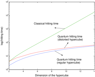
Figure 4: Comparison of hitting times on the regular and distorted hypercubes

Figure 4 plots the hitting time of a quantum walk on a distorted hypercube together with that of a classical walk and a quantum walk on regular hypercubes for comparison. The hitting time for a quantum walk on a distorted hypercube is more than that of a quantum walk on a regular hypercube, but still is much smaller than the hitting time of a classical walk. In fact, as the dimension increases one can see that the hitting times of the quantum walk on the distorted and regular hypercubes converge towards each other. This presumably reflects the fact that for higher dimensions the symmetry is mostly unchanged.

V Conclusions

We have examined the definition of hitting time for measured quantum walks and analyzed some of its properties. We used this definition to obtain an expression for hitting time which is valid on any general graph as long as the unitary evolution operator $\hat{U}$ of the walk is defined. We simulated this hitting time for a measured quantum walk using the Grover coin and compared it to the classical hitting time and to the bounds obtained on it; the quantum hitting time is exponentially smaller than the classical hitting time. We also showed that the bounds on the hitting time obtained in kempe_comp become less tight as the dimension increases.

However, simply making a walk quantum does not guarantee a speed-up over the classical case. We demonstrated that the hitting time for quantum walks can depend sensitively on the initial condition, unlike classical walks. For certain initial states, the DFT walk can have infinite hitting time, a phenomenon not possible in classical random walks. This dependence on the initial state varies with the coin used, since for the same initial state the Grover walk has a polynomial hitting time. This infinite hitting time is directly related to the degeneracy of the eigenvalues of the evolution operator. If the evolution operator is highly degenerate, then it is very likely that there exist initial states which give infinite hitting times.

While the exact cause of the speed-up in quantum hitting time is not completely clear, it seems very likely that the symmetry of the graph plays a major role in both the speed-up and slow down of the quantum walk. In the faster quantum walk, the different paths leading to the final vertex interfere constructively, enhancing the probability of arrival; paths which lead to “wrong” vertices interfere destructively, reducing the probability of meandering around in the graph for long times. Unlike a classical random walk, the quantum walk is sensitive to the presence of a global symmetry which is not apparent at a purely local level. This phenomenon probably leads to the speed-up of the continuous-time quantum walk on the glued-trees graph as well childs2 .

However, this same symmetry is undoubtedly the culprit in the slow-down observed for the DFT walk. The existence of states which never arrive at the final vertex is made possible by the degeneracy of the evolution operator $\hat{U}$—a degeneracy which arises due to the symmetry of the graph. The existence of states which never arrive at the final vertex can also be seen as an interference effect, only in this case the interference of paths which lead to the final vertex is destructive: all amplitude to make a transition to the final vertex cancels out.

This interpretation is supported by the quantum walk on the distorted hypercube. We observe that the hitting time is worse than that of the usual hypercube, but still much smaller than that of a classical walk. The curve of the hitting time on the distorted hypercube seems to converge slowly to that of a quantum walk on the regular hypercube. This is probably because the distortion (described in section 4) is very mild. As the dimension grows, and with it the number of edges and vertices, this distortion has less effect on the overall symmetry.

We hasten to add that symmetry of the graph is not the sole reason for speed-ups in quantum walks. A polynomial speed-up has been demonstrated in the quantum walk versions of the search of an unstructured database shenvi and the element distinctness problem ambainisApp . However, the dramatic exponential speed-ups have all been demonstrated in highly symmetric graphs.

This suggests that the most promising direction to look for new algorithms based on quantum walks is for problems which possess a global symmetry, but for which this symmetry is not apparent at the level of individual candidate solutions. Yet even for such a problem, care will have to be taken if quantum mechanics is to serve as a blessing and not as a curse.

References

- (1) R. Motwani and P.Raghavan, Randomized Algorithms (Cambridge University Press, Cambridge, 1995).
- (2) P.W. Shor, in Proceedings of the 35th Annual Symposium on the Theory of Computer Science, edited by S. Goldwasser, 124 (IEEE Computer Society Press, Los Alamitos, CA, 1994).
- (3) E. Farhi and S. Gutmann, Phys, Rev. A 58, 915 (1998).
- (4) A.M. Childs, E. Farhi and S. Gutmann, Quantum Information Processing 1, 35 (2002).
- (5) A.M. Childs, R. Cleve, E. Deotto, E. Farhi and D.A. Spielman, Exponential algorithmic speedup by quantum walk (2002), in Proc. 35th ACM Symposium on Theory of Computing (STOC 2003), (ACM Press, New York, 2003), 59–68.
- (6) A. Nayak and A. Vishwanath. Quantum walk on the line,
- (7) E. Bach, S. Coppersmith, M. Goldschen, R. Joynt and J. Watrous, One-dimensional quantum walks with absorbing boundaries, Journal of Computer and System Sciences 69, 562–592 (2004).
- (8) T.A. Brun, H.A. Carteret and A. Ambainis. The quantum to classical transition for random walks, Phys. Rev. Lett. 91, 130602 (2003).
- (9) T.A. Brun, H.A. Carteret and A. Ambainis, Quantum random walks with decoherent coins, Phys. Rev. A 67, 032304 (2003).
- (10) T.A. Brun, H.A. Carteret and A. Ambainis, Quantum walks driven by many coins, Phys. Rev. A 67, 052317 (2003).
- (11) Julia Kempe, Quantum random walks hit exponentially faster, in Proc. 7th Intern. Workshop on Randomization and Approximation Techniques in Computer Science (RANDOM’03), edited by S. Arora, K. Jansen, J.D.P. Rolim and A. Sahai (Springer, Berlin, 2003), 354–69.
- (12) Neil Shenvi, Julia Kempe and K. Brigitta Whaley, A quantum random walk search algorithm, Phys. Rev. A 67, 052307 (2003).
- (13) C. Moore and A. Russell, in Proc. 6th Intl. Workshop on Randomization and Approximation Techniques in Computer Science (RANDOM ’02), edited by J. D. P. Rolim and S. Vadhan (Springer, Berlin, 2002), 164–178.
- (14) D. Aharanov, A. Ambainis, J. Kempe and U. Vazirani, in Proc. 33rd Annual ACM Symposium on Theory of Computing (STOC 2001) (Assoc. for Comp. Machinary, New York, 2001) pp. 50–59.
- (15) A. Ambainis, Quantum walks and their algorithmic applications, Intl. J. Quantum Information 1, 507 (2003).
- (16) V. Kendon, Quantum walks on general graphs, quant-ph/0306140.
- (17) A. Ambainis, in Proceedings of 45th Annual IEEE Symposium on Foundations of Computer Science (FOCS 2004) (IEEE Computer Society Press, Los Alamitos, CA, 2004), 22–31.
- (18) J. Kempe, Quantum random walks-an introductory overview, Contemp. Phys. 44 (2003).
- (19) W.E. Roth, Bull. Amer. Math. Soc. 40, 461 (1934).
- (20) G. Alagić and A. Russell, Decoherence in Quantum Walks on the Hypercube, quant-ph/0501169.