A fault-tolerant one-way quantum computer

We describe a fault-tolerant one-way quantum computer on cluster states in three dimensions. The presented scheme uses methods of topological error correction resulting from a link between cluster states and surface codes. The error threshold is 1.4% for local depolarizing error and 0.11% for each source in an error model with preparation-, gate-, storage- and measurement errors.

1 Introduction

A quantum computer as a physical device has to cope with imperfections of its hardware. Fortunately, it turns out that arbitrary large quantum computations can be performed with arbitrary accuracy, provided the error level of the elementary components of the quantum computer is below a certain threshold. This is the content of the threshold theorem for quantum computation [1, 2, 3, 4]. The threshold theorem also provides lower bounds to the error threshold which are in the range between $10^{-10}$ and $10^{-4}$, depending on the error model. It thus appears that there is a gap between the required and the currently available accuracy of quantum operations, and it invites narrowing from both the experimental and the theoretical side. In this context, significant progress has been made in [5] where a threshold estimate in the percent range has been demonstrated. For experimentally viable quantum computation there is a further desideratum besides a high error threshold. With the exception of certain schemes for topological quantum computation [6, 7, 8], the price for fault-tolerance is an overhead in quantum resources. This overhead should be moderate.

Here we describe a fault-tolerant version of the one-way quantum computer ($QC_{\cal{C}}$). The $QC_{\cal{C}}\;$is a scheme for universal quantum computation by one-qubit measurements on cluster states [9]. Cluster states [10] consist of qubits arranged on a two- or three-dimensional lattice and may be created by a nearest-neighbor Ising interaction. Thus, for the $QC_{\cal{C}}$, only nearest-neighboring qubits need interact and furthermore, only once at the beginning of the computation. For this scenario in three dimensions we present methods of error correction and a threshold value.

The existence of an error threshold for the $QC_{\cal{C}}\;$has previously been established [11, 12, 13] and threshold estimates have been obtained [12, 13], by mapping to the circuit model. Here we take a different path. We make use of topological error correction capabilities that the cluster states naturally provide [14] and which can be linked to surface codes [6, 15]. The main design tool upon which we base our construction are engineered lattice defects which are topologically entangled.

The picture is the following: quantum computation is performed on a three-dimensional cluster state via a temporal sequence of one-qubit measurements. The cluster lattice is subdivided into three regions, $V$, $D$ and $S$. The set $S$ comprises the ‘singular’ qubits which are measured in an adaptive basis. The quantum computation happens essentially there. The sets $V$ and $D$ are to distribute the correct quantum correlations among the qubits of $S$. $V$ stands for ‘vacuum’, the quantum correlations can propagate and spread freely in $V$. $D$ stands for ‘defect’. Quantum correlations cannot penetrate the defect regions. They either end in them or wrap around them. In both cases, the defects guide the quantum correlations. $V$ and $D$ are distinguished by the bases in which the respective cluster qubits are measured. The region $V$ fills most of the cluster. Embedded in $V$ are the defects ($D$) most of which take the shape of loops. These loops are topologically entangled with another. Further, there are defects in the shape of ear clips which each hold an $S$-qubit in their opening. Such a defect and the belonging $S$-qubit form again a loop. These are the only locations where the $S$-qubits occur. See Fig. 1.

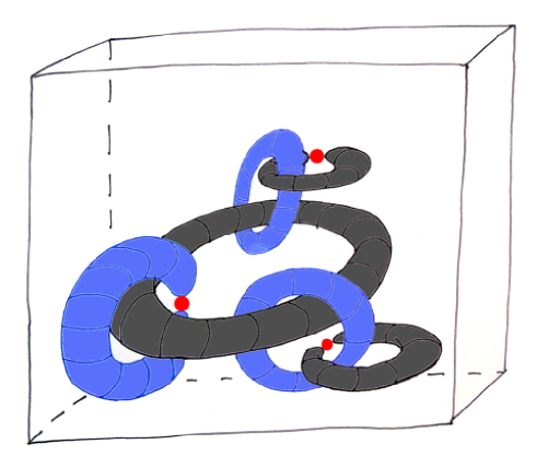
Figure 1: Topological error correction for the $QC_{\cal{C}}$. The three-dimensional cluster state, shown as a block, is structured by lattice defects which exist in two kinds: primal and dual. The defects wind around another. Some of them hold singular qubits (red) which realize the non-Clifford part of the quantum computation.

There are two codes upon which we base our construction, the planar code [15] and the concatenated $[15,3,1]$ quantum Reed-Muller code [16, 17]. Both codes individually have their strengths and weaknesses, but they can be advantageously combined. The planar code has a relatively high error threshold of about 11% [18], and the symmetries of its stabilizer fit well with cluster states. Moreover, fault-tolerant data storage with the planar code and the creation of long range entanglement among planar code qubits are easily accomplished in three-dimensional cluster states, via a bcc-symmetric pattern of one-qubit measurements. Therefore, it is suggestive to base fault-tolerant cluster state computation on this code. However, the planar code is not well suited to non-Clifford operations which are essential for universal quantum computation.

Now, in cluster- and graph state quantum computation, the non-Clifford part of the circuit is implemented by destructive measurements of the observables $(X\pm Y)/\sqrt{2}$ (The Clifford part is implemented by $X$-, $Y$- and $Z$-measurements.). The Reed-Muller quantum code is well suited for fault-tolerant quantum computation via local measurements because the measurements of the encoded observables $(\overline{X}\pm\overline{Y})/\sqrt{2}$ (and of $\overline{X}$, $\overline{Y}$, $\overline{Z}$ besides) are accomplished fault-tolerantly by the respective measurements on the bare level—and bare level measurements is what we are allowed to do in the $QC_{\cal{C}}$. If we could assume we had given a graph state state as algorithmic resource where each cluster qubit was encoded with the concatenated Reed-Muller code and where noise acted locally on the bare level, then fault-tolerant quantum computation were trivial to achieve. However, is not obvious how to create such an encoded graph state affected by local noise only. But this is just what the topological error correction in cluster states can do.

This paper is organized as follows. In Section 2, we introduce the ingredients required for the error correction mechanisms we use, namely cluster states, the planar code and the 15-qubit Reed-Muller quantum code. In Section 3 the measurement pattern used for fault-tolerant cluster state quantum computation is described, and in Sections 5 - 6 it is explained. Specifically, in Section 5 we describe the physical objects relevant for the discussed scheme—defects, cluster state quantum correlations, errors and syndrome bits—in the language of homology. In Section 6 we introduce the techniques for structuring quantum correlations via topological entanglement of lattice defects. Our error models are stated in Section 7.1 and the fault-tolerance threshold is derived in Section 7.2. The overhead is estimated in Section 8. We discuss our results in Section 9.

2 Cluster states and quantum codes

This section is a brief review of the ingredients for the described fault-tolerant $QC_{\cal{C}}$.

Cluster states.

A cluster state is a stabilizer state of qubits, where each qubit occupies a site on a $d$-dimensional lattice ${\cal{C}}$. Each site $a\in{\cal{C}}$ has a neighborhood $N(a)$ which consists of the lattice sites with the closest spatial distance to $a$. Then, the cluster state $|\phi\rangle_{\cal{C}}$ is—up to a global phase—uniquely defined via the generators $K_{a}$ of its stabilizer

$$K_{a}:=X_{a}\bigotimes_{b\in N(a)}Z_{b},\;\;\forall a\in{\cal{C}},$$ (1)

i.e., $|\phi\rangle_{\cal{C}}=K_{a}|\phi\rangle_{\cal{C}}$. Here, $X_{a}$ and $Z_{b}$ are a shorthand for the Pauli operators $\sigma_{x}^{(a)}$ and $\sigma_{z}^{(b)}$ that we use throughout the paper. We refer to the generators $K_{a}$ of the cluster state stabilizer as the elementary cluster state quantum correlations.

In this paper, we will use as the lattice underlying the cluster state a bcc-symmetric lattice in tree dimensions. That is, the location of cluster qubits is given by lattice vectors

$$\begin{array}[]{lcr}\{(o\mbox{[dd]},e\mbox{[ven]},e),(e,o,e),(e,e,o)\},&&\mbox{odd qubits},\\ \{(e,o,o),(o,e,o),(o,o,e)\},&&\mbox{even qubits}.\end{array}$$ (2)

We sub-divide the set of qubits into two subsets, the even and the odd qubits. For even (odd) qubits the sum of the coordinates of their respective lattice site is even (odd).

Note that instead of with a bcc-symmetric lattice we could have equivalently started with a cluster state on an sc-symmetric lattice, because a cluster state on the latter is mapped to a cluster state on the former by $Z$-measurements on the qubits $(e,e,e)$ and $(o,o,o)$; see [9].

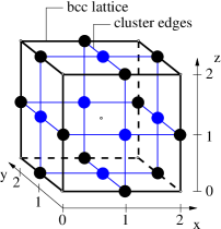
Figure 2: Elementary cell of the bcc lattice. Qubits live on the faces and edges of the elementary cell. Syndrome bits are located in the cube and on the sites. Each elementary cell has a volume of $2\times 2\times 2$ in cluster units. Black: elementary cell of the bcc lattice, blue: edges of the cluster graph.

The $[15,3,1]$ quantum Reed-Muller code.

By this we denote a 15 qubit CSS-code based on the (classical) punctured Reed-Muller code ${\cal{R}}(1,4)^{*}$ [19]. Its stabilizer generator matrix has the form

$$G_{RM}=\left(\begin{array}[]{c|c}G_{X}&0\\ 0&G_{Z}\end{array}\right),$$ (3)

where

$$G_{X}=\left(\begin{array}[]{lllllllllllllll}1&0&1&0&1&0&1&0&1&0&1&0&1&0&1\\ 0&1&1&0&0&1&1&0&0&1&1&0&0&1&1\\ 0&0&0&1&1&1&1&0&0&0&0&1&1&1&1\\ 0&0&0&0&0&0&0&1&1&1&1&1&1&1&1\end{array}\right),$$ (4)

and $G_{Z}$ is given by ${G_{X}}^{\perp}=G_{Z}\oplus(1,1,...,1,1)$.

This code has the fairly rare property that the encoded non-Clifford gate $\overline{U}_{z}(\pi/4)=\exp(-i\pi/8\overline{Z})$ is local [16, 17], i.e.,

$$\exp\left(-i\frac{\pi}{8}\,\overline{Z}\right)\cong\bigotimes_{i=1}^{15}\exp\left(i\frac{\pi}{8}\,Z_{i}\right).$$ (5)

This property has been used in magic state distillation [17]. In the computational scheme described here we use it to fault-tolerantly measure the encoded observables $\frac{\overline{X}\pm\overline{Y}}{\sqrt{2}}$ via local measurements of observables $\frac{X_{i}\pm Y_{i}}{\sqrt{2}}$.

Surface codes.

For the surface codes [6, 15] physical qubits live on the edges of a two-dimensional lattice. The support of a physical error must stretch across a constant fraction (typically 1/2) of the lattice to cause a logical error. The protection against errors is topological.

The stabilizer generators of the code are associated with the faces $f$ and the vertices $v$ of the lattice,

$$S_{X}(v)=\bigotimes_{e|\,v\in\{\partial e\}}X_{e},\;\;S_{Z}(f)=\bigotimes_{e\in\{\partial f\}}Z_{e}.$$ (6)

Therein, $\partial$ is the boundary operator. The number of qubits that can be stored depends on the boundary conditions of the code lattice. The code resulting from periodic boundary conditions, the ‘toric code’ [6], can store two qubits.

As an example we would briefly like to discuss the planar code [15] which encodes one qubit; see Fig. 3a. This example exhibits many features of our subsequent constructions one dimension higher up: Errors are identified with 1-chains and show a syndrome only at their end points. Homologically equivalent chains correspond to physically equivalent errors. Error chains can end in the system boundary without leaving a syndrome.

Specifically, Pauli operators $Z_{i}$ live on the edges of the primal (=shown) lattice, and Pauli operators $X_{j}$ live on edges of the dual lattice. The encoded $Z$-operator is a tensor product of individual $Z_{i}$ operators corresponding to a primal 1-chain stretching from left to right across the code lattice. The encoded $X$-operator corresponds to a 1-chain of the dual lattice that stretches from top to bottom.

The code stabilizer is modified at the system boundary. For example, a face to the left or right of the lattice has only three elementary 1-chains in its boundary, instead of four. Such boundary is called a ‘rough edge’. Where no modification of the faces occurs the system boundary is a ‘smooth edge’. ‘Smooth’ on the primal lattice is ‘rough’ on the dual, and vice versa. Error chains can end in a rough edge of their respective lattice without leaving a syndrome, but not in a smooth edge.

The surface codes will occur rather implicitly in our constructions. The reason is that here we do not use such codes to encode logical qubits. Instead, we use them to appropriately “wire” a subset of the cluster qubits, the $S$-qubits. The link between surface codes and cluster states has been established in [14], for the purpose of creating long range entanglement in noisy 3D cluster states via local measurements. It has been found that the error correction implemented by the local measurements is described—like fault-tolerant data storage with the toric code—by the so-called Random plaquette $\mathbb{Z}_{2}$-gauge model in three dimensions (RPGM) [18]. The three-dimensional cluster state is like a surface code, one dimension higher up. The third dimension, which is temporal in data storage with the toric code, is spatial for the cluster state. The extra spatial dimension can be used to fault-tolerantly mediate interaction among qubits. The creation of an encoded Bell state over large distances [14] is the simplest example. The long-range quantum correlations are engineered by the suitable choice of boundary conditions.

Why are the above two codes chosen? For the fault-tolerant scheme of quantum computation described in this paper we require a quantum code with the following three properties: 1) The code is of CSS-type, 2) The code satisfies Eq. (5), and 3) The code fits with cluster states. For some arrangement of qubits on a translation-invariant two-dimensional lattice, the code has a translation-invariant set of stabilizer generators and these generators each have a small support on the lattice.

The Reed-Muller code has properties 1 and 2 but not 3. The surface codes have properties 1 and 3 but not 2. Thus, neither of the codes alone suffices. But their combination does, as is described in the subsequent sections.

a)	b)

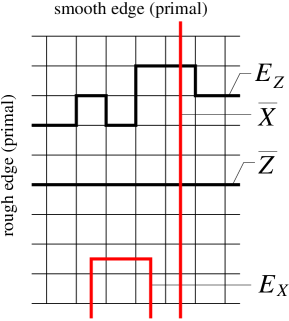
Figure 3: Codes. a) Planar code. The encoded Pauli observables $\overline{X}$ and $\overline{Z}$, two errors and the different boundary types ‘smooth’ and ‘rough’ are shown. The errors $E_{X}$, $E_{Z}$ end in their respective rough boundary. $E_{X}$ corresponds to a trivial 1-cycle on the dual lattice and has no effect on the encoded state. $E_{Z}$ corresponds to an non-trivial 1-cycle on the primal lattice. It leaves no syndrome but causes a logical $Z$-error. b) Bi-colorable graph state locally unitary equivalent to the $\overline{|+\rangle}$-state of the 15-qubit quantum Reed-Muller code.

3 The measurement pattern

As pointed out in the introduction, we subdivide the cluster $C$ into the three disjoint subsets $V$, $D$ and $S$. $S$ is the the set of qubits where the non-Clifford part of the quantum computation is performed, and $V$ and $D$ are to connect the qubits of $S$ in the proper way. We have not yet explained what the defects are, and we will do so only in the next section. For the moment it suffices to note that the defects are located on the subset $D$ of the cluster, and that $D$ is the union of the two disjoint subsets $D_{1}$ and $D_{2}$. The measurement pattern on $D$, $S$ and $V$ is given by

$$\begin{array}[]{lll}\mbox{Defect qubits}\,\,a\in D:&\mbox{Measurement of }\left\{\begin{array}[]{r}X_{a}\\ Z_{a}\end{array}\right.,&\mbox{if}\,\,\left\{\begin{array}[]{r}a\in D_{2}\\ a\in D_{1}\end{array}\right.,\vspace{1mm}\\ \mbox{Singular qubits}\,\,a\in S:&\mbox{Measurement of }\displaystyle{\frac{X_{a}\pm Y_{a}}{\sqrt{2}}},\vspace{1mm}\\ \mbox{Vacuum qubits}\,\,a\in V:&\mbox{Measurement of}\,\,X_{a}.\end{array}$$ (7)

Now we have to explain why we choose this measurement pattern, which is best done using the language of homology.

4 Involving the Reed-Muller quantum code

In this section we explain the role of the Reed-Muller code for the described computational scheme. Consider a cluster state $|\phi\rangle_{{\cal{C}}_{2}}$ on a two-dimensional cluster ${\cal{C}}_{2}$. It is a resource for universal quantum computation by measurements of the local observables $X$, $Z$ and $\frac{X\pm Y}{\sqrt{2}}$, [9]. Denote by $Q\subset{\cal{C}}_{2}$ the set of qubits which are measured in the eigenbasis of $\frac{X\pm Y}{\sqrt{2}}$. These measurements implement the non-trivial part of a quantum circuit. The measurements of $X$ and $Z$ on the qubits ${\cal{C}}_{2}\backslash Q$ implement the Clifford part. They are performed simultaneously in the first round of measurements. $|\Psi_{\text{algo}}\rangle_{Q}$ is the state of the unmeasured qubits after the first measurement round. It is an algorithm-specific stabilizer state, hence the subscript “algo”. Since it is a stabilizer state, it is easy to create and one may start with this state as an algorithm-specific resource instead of the universal cluster state. Quantum computation with this state proceeds by measuring local observables $\frac{X\pm Y}{\sqrt{2}}$.

Now suppose an encoded version of this state, $|\overline{\Psi}_{\text{algo}}\rangle_{S}$, was given. The state were not perfect but only affected by local noise on the bare level. Of course, a question that arises immediately is how such a state is obtained. The main part of work in this paper goes into answering this question, see subsequent sections. Now, with $|\overline{\Psi}_{\text{algo}}\rangle_{S}$ given, one could perform fault-tolerant quantum computation by fault-tolerant measurement of the encoded observables $\frac{\overline{X}\pm\overline{Y}}{\sqrt{2}}$. This is not what we have in mind, because we are seeking a scheme of fault-tolerant quantum computation by local measurements. Here lies the reason for involving the (concatenated) Reed-Muller code: For this code, the fault-tolerant measurement of the observables $\frac{\overline{X}\pm\overline{Y}}{\sqrt{2}}$ proceeds by local measurements of observables $\frac{X\pm Y}{\sqrt{2}}$. The reason for this is property (5). If $J$ is a set such that $g_{X}(J):=\bigotimes_{j\in J}X_{j}$ is in the RM code stabilizer, then also

$$g_{\pm}(J):=\bigotimes_{j\in J}\frac{X_{j}\pm Y_{j}}{\sqrt{2}}\in\mbox{RM code stabilizer}.$$ (8)

The relevant encoded observables are given by

$$\frac{\overline{X}\pm\overline{Y}}{\sqrt{2}}=\bigotimes_{j}\frac{X_{j}\mp Y_{j}}{\sqrt{2}}.$$ (9)

The “$\mp$” is for the total number of concatenation levels being odd. If the number is even, replace “$\mp$” by “$\pm$”. Therefore, if all the bare qubits belonging to an encoded qubit are individually measured in the eigenbasis of $\frac{X_{j}-Y_{j}}{\sqrt{2}}$, then the eigenvalue found in a measurement of the encoded observable $\frac{\overline{X}+\overline{Y}}{\sqrt{2}}$ and the eigenvalues of the stabilizer generators $g_{+}(J)$ can be deduced from the individual measurement outcomes. This is all what is needed for fault-tolerant measurement of the encoded observable $\frac{\overline{X}+\overline{Y}}{\sqrt{2}}$.

The $Z$-part of the code stabilizer is lost in the local measurement, but it is not needed for the fault-tolerant measurement of $\frac{\overline{X}\pm\overline{Y}}{\sqrt{2}}$. This can be seen as follows. For simplicity assume a local depolarizing error $p/3\left([X_{j}]+[Y_{j}]+[Z_{j}]\right)=\frac{p}{3\sqrt{2}}\left(\left[X_{j}+Y_{j}\right]+\left[X_{j}-Y_{j}\right]+\sqrt{2}[Z_{j}]\right)$ for all qubits $j$. The brackets “$[\cdot]$” indicate a super-operator. W.l.o.g. assume that the local measurements are in the eigenbasis of $\frac{X_{j}-Y_{j}}{\sqrt{2}}$. Then, the error $\frac{X_{j}-Y_{j}}{\sqrt{2}}$ is absorbed in the measurement and has no effect. The second error $\frac{X_{j}+Y_{j}}{\sqrt{2}}=i\frac{X_{j}-Y_{j}}{\sqrt{2}}Z_{j}\cong Z_{j}$, so all remaining errors are equivalent to $Z$-errors. Such errors are identified by the stabilizer elements $\{g_{+}(J)\}$.

To summarize, the Reed-Muller code is involved to perform the fault-tolerant measurement of the encoded observables locally on the bare level. The eigenvalues corresponding to the encoded observable and to the relevant stabilizer generators are simultaneously inferred from the measurement outcomes. Error correction proceeds by classical post-processing of these quantities.

5 Involving a topological quantum code - Homology

The remaining question is how we actually create the state $|\overline{\Psi}_{\text{algo}}\rangle_{S}$ with only local error from a three-dimensional cluster state. To accomplish this task we involve topological error correction.

5.1 Errors and correlations as chains

The physical objects of our discussion—cluster state correlations and error operators—may be identified with faces and edges of an underlying lattice. Compositions of such faces or edges are called 2-chains and 1-chains, respectively. For the chains homology provides an equivalence relation; namely, two chains are homologically equivalent if they differ by the boundary of a third chain one dimension higher up [20, 21, 22]. Homology plays a role in our constructions because homological equivalence of the underlying chains implies physical equivalence of the associated physical objects.

First we introduce the two simple cubic sub-lattices ${\cal{L}}$ and $\overline{\cal{L}}$ whose vertices are at locations

$$\begin{array}[]{rcl}{\cal{L}}&:&\{(e,e,e)\},\\ \overline{\cal{L}}&:&\{(o,o,o)\}.\end{array}$$ (10)

One lattice can be obtained from the other via translation by a vector $(\pm 1,\pm 1,\pm 1)$. ${\cal{L}}$ and $\overline{\cal{L}}$ are dual to another in the sense that the faces of ${\cal{L}}$ are the edges of $\overline{\cal{L}}$, the cubes of ${\cal{L}}$ are the vertices of $\overline{\cal{L}}$, and vice versa. We denote by $*$ the duality transformation that maps primal edges into the corresponding dual faces ($*e=\overline{f}$), and so forth.

We denote by ${\cal{B}}(C_{0}):=\{v_{k}\}$ the set of vertices in ${\cal{L}}$, by ${\cal{B}}(C_{1})=\{e_{l}\}$ the set of edges in ${\cal{L}}$, by ${\cal{B}}(C_{2})=\{f_{m}\}$ the set of faces in ${\cal{L}}$, and by ${\cal{B}}(C_{3})=\{q_{n}\}$ the set of elementary cells [or cubes] of ${\cal{L}}$. We may now define chains in ${\cal{L}}$ [20]. ${\cal{B}}(C_{0})$ forms a basis for the set $C_{0}$ of so called 0-chains $c_{0}$, ${\cal{B}}(C_{1})$ forms a basis for the set $C_{1}$ of 1-chains $c_{1}$, and so forth. Specifically, the chains are given by

$$\begin{array}[]{rclcrclcrclcrcl}c_{0}&=&\sum_{k}z_{k}v_{k},&c_{1}&=&\sum_{l}z_{l}e_{l},&c_{2}&=&\sum_{m}z_{m}f_{m},&c_{3}&=&\sum_{n}z_{n}q_{n}.\end{array}$$ (11)

where $z_{k},z_{l},z_{m},z_{n}\in\mathbb{Z}_{2}$. The sets $C_{0}$, $C_{1}$, $C_{2}$ and $C_{2}$ are, in fact, abelian groups under component-wise addition, e.g. $c_{1}+c_{1}^{\prime}=\sum_{l}z_{l}e_{l}+\sum_{l}z_{l}^{\prime}e_{l}=\sum_{l}(z_{l}+z_{l}^{\prime})e_{l}$. For each $i=1..3$, there exists a homomorphism $\partial_{i}$ mapping $C_{i}$ to $C_{i-1}$, with the composition $\partial_{i-1}\circ\partial_{i}=0$. Then,

$${\cal{L}}=\{C_{3},C_{2},C_{1},C_{0}\}$$ (12)

is called a chain complex, and $\partial$ is called boundary operator. It maps an $i$-chain $c_{i}$ to its boundary, which is an $i-1$-chain. In the same way, $\overline{\cal{L}}$ can be defined as a dual chain complex, $\overline{\cal{L}}=\{\overline{C}_{3},\overline{C}_{2},\overline{C}_{1},\overline{C}_{0}\}$, with chains $\overline{c}_{3}$, $\overline{c}_{2}$, $\overline{c}_{1}$ and $\overline{c}_{0}$.

Now, considering a space ${\cal{C}}$, two chains $c_{n},\,c_{n}^{\prime}\in C_{n}({\cal{C}})$ are homologically equivalent if $c_{n}^{\prime}=c_{n}+\partial c_{n+1}$ for some $c_{n+1}\in C_{n+1}({\cal{C}})$ [20]. Of interest for topological error-correction is the notion of relative homology. Consider a pair of spaces $({\cal{C}},D)$ with $D\subset{\cal{C}}$. Then, two chains $c_{n}$, $c_{n}^{\prime}$ are called equivalent w.r.t relative homology, $c_{n}^{\prime}\cong_{\text{r}}c_{n}$, if $c_{n}^{\prime}=c_{n}+\partial c_{n+1}+\gamma_{n}$ for some $c_{n+1}\in C_{n+1}({\cal{C}})$, $\gamma_{n}\in C_{n}(D)$; see [21]. Relative cycles may end in $D$.

Below we describe how the cluster state quantum correlations may be identified with the 2-chains, the errors with the 1-chains and the syndrome with the 0-chains of ${\cal{L}}$ and $\overline{\cal{L}}$. All these objects appear in two kinds, ‘primal’ and ‘dual’, depending on whether they are defined with respect to ${\cal{L}}$ or $\overline{\cal{L}}$.

Cluster state correlations.

We define primal such correlations, $K(c_{2})$, and dual ones, $K(\overline{c}_{2})$, which can be identified with 2-chains in ${\cal{L}}$ and $\overline{\cal{L}}$, respectively, by

$$K(c_{2}):=\prod_{f\in\{c_{2}\}}K_{f},\;\;K({\overline{c}_{2}}):=\prod_{\overline{f}\in\{\overline{c}_{2}\}}K_{\overline{f}}.$$ (13)

Therein, e.g. the set $\{c_{2}\}$ is defined via a mapping $c_{2}=\sum_{m}z_{m}f_{m}\longrightarrow\{c_{2}\}=\{f_{m}|z_{m}=1\}$. Further, we introduce the notion $O(c):=\bigotimes_{a\in\{c\}}O_{a}$, for all $c\in C$ and $O\in\{X,Z\}$. It is now easily verified that

$$K(c_{2})=X(c_{2})Z(\partial c_{2}),\;K(\overline{c}_{2})=X(\overline{c}_{2})Z(\partial\overline{c}_{2}).$$ (14)

Errors.

We will mainly discuss (correlated) probabilistic noise. Then, it is sufficient to restrict the attention to Pauli phase flips $Z$, because $X_{a}\cong\bigotimes_{b\in N(a)}Z_{b}$ etc. We combine $Z$-errors on odd (even) qubits to primal (dual) error chains $E(c_{1})$ ($E(\overline{c}_{1})$),

$$E(c_{1}):=Z(c_{1}),\;\;E(\overline{c}_{1}):=Z(\overline{c}_{1}).$$ (15)

Syndrome.

The first type of correlations we discuss are those for error correction in $V$. They are characterized by the property that the corresponding 2-chains have no boundary. I.e., we consider $K(c_{2})$, $K(\overline{c}_{2})$ with $\{c_{2}\},\{\overline{c}_{2}\}\in V$ and $\partial c_{2}=\partial\overline{c}_{2}=0$. With (13), these correlations take the form $K(c_{2})=X(c_{2})$, $K(\overline{c}_{2})=X(\overline{c}_{2})$. They are measured by the $X$-measurements in $V$, see (7), and are used to identify errors occurring on the qubits $\{c_{2}\}$, $\{\overline{c}_{2}\}$.

The group of 2-chains in the kernel of $\partial$ we denote by $Z_{2}({\cal{L}})$. Since $\partial\partial=0$, a subgroup of those, $B_{2}({\cal{L}})$, is formed by the 2-chains which are themselves a boundary of a 3-chain. Denote by $q$ ($\overline{q}$) a 3-chain from the basis ${\cal{B}}(C_{3})$ (${\cal{B}}(\overline{C}_{3})$). It represents an individual cell [or cube] of the primal lattice ${\cal{L}}$ (dual lattice $\overline{\cal{L}}$). The associated quantum correlations are

$$K_{q}:=K(\partial q)=X(\partial q),\;\;K_{\overline{q}}:=K(\partial\overline{q})=X(\partial\overline{q}).$$ (16)

When being measured, each of these correlations yields a syndrome bit $Sy(q)$, $Sy(\overline{q})$ which, we say, is located at $q$ or $\overline{q}$, respectively. Because the lattices ${\cal{L}}$ and $\overline{\cal{L}}$ are dual to another, we may identify the cell $q$ in ${\cal{L}}$ with a vertex $\overline{v}$ in $\overline{\cal{L}}$, and vice versa. In this way, the syndrome bits become located at vertices of the lattices ${\cal{L}}$ and $\overline{\cal{L}}$. The syndrome resulting from the quantum correlations (16) are those which enable topological error correction [18].

Syndrome and errors.

Let $E(c_{1})$ denote a primal error chain, $\overline{q}\in{\cal{B}}(\overline{C}_{3})$ a cell in the dual lattice $\overline{\cal{L}}$ and $v\in{\cal{B}}(C_{0})=*\overline{q}$. $K(\overline{q})$ detects the error $E(c_{1})$ if $|\{c_{1}\}\cap\{\partial\overline{q}\}|=\mbox{odd}$. Equivalently, $K(\overline{q})$ detects $E(c_{1})$ if $v\in\{\partial c_{1}\}$. Thus, error chains show a syndrome only at their ends.

Correlations and errors.

Primal cluster state correlations are affected by dual error chains and dual correlations are affected by primal error chains. Primal correlations are not affected by primal error chains, and dual correlations are not affected by dual error chains.

To see this, note that a primal correlation $K(c_{2})$ consists of Pauli operators $X$ on even qubits and Pauli operators $Z$ on odd qubits. A dual error chain $E(\overline{c}_{1})$ consists of operators $Z$ on even qubits. Then, $E(\overline{c}_{1})K(c_{2})=(-1)^{|\{\overline{c}_{1}\}\cup\{c_{2}\}|}\,K(c_{2})E(\overline{c}_{1})$. If $|\{\overline{c}_{1}\}\cup\{c_{2}\}|$ is odd, the correlation $K(c_{2})$ is conjugated to $-K(c_{2})$ by the error. If it is even, then the correlation remains unchanged. This situation has a geometric interpretation. $|\{\overline{c}_{1}\}\cup\{c_{2}\}|$ is the number of intersection points between the primal 2-chain $c_{2}$ and the dual 1-chain $\overline{c}_{1}$. If the number of intersections is odd (even) then the correlation is (is not) affected by the error. For dual correlations and primal errors the situation is the same. Further, a primal error chain consists of Pauli operators $Z$ on odd qubits. Thus, $[K(c_{2}),E(c_{1})]=0$ always. Similarly, $[K(\overline{c}_{2}),E(\overline{c}_{1})]=0$, $\forall\,\overline{c}_{1},\overline{c}_{2}$.

Defects.

The purpose of defects is to structure the space underlying the pair of lattices ${\cal{L}},\overline{\cal{L}}$. Practically, a defect can be thought of as a set of qubits that are removed from the initial cluster ${\cal{C}}$ before the remaining qubits are entangled. For the chain complexes $C$, $\overline{C}$, a defect is a set $d$ of missing edges. What defines a defect as an entity is that the belonging edges are connected. As all the other objects, defects are either primal or dual,

$$d\subset{\cal{B}}(C_{1}),\;\overline{d}\subset{\cal{B}}(\overline{C}_{1}).$$ (17)

The sets $d$, $\overline{d}$ of defect qubits are not arbitrary. Seen from afar they take the shape of doughnuts. These doughnut-shaped defects will be topologically entangled with another, and the way they are entangled encodes the quantum algorithm to be performed. From the viewpoint of quantum logic, what matters about the doughnuts is that they are loops. Their ‘thickness’ is required for fault-tolerance.

We now briefly explain how the above definition of a defect as a set of missing cluster qubits fits with the measurement pattern (7). Formally, each defect $d$ will be assigned a set $D(d)$ of locations on the cluster. This set is subdivided into a set of edge- and a set of face qubits, $D_{1}(d)$ and $D_{2}(d)$. Here, the notions of ‘edge’ and ‘face’ are in reference to the lattice the defect belongs to. If the defect is primal (dual) then the edges and faces are taken with respect to the primal (dual) lattice. For primal defects, the sets $D_{1}(d)$ and $D_{2}(d)$ are defined as

$$D_{1}(d):=d,\;D_{2}(d)=\left\{f\in{\cal{B}}(C_{2})|\,\{\partial f\}\cap d=\{\partial f\}\right\}.$$ (18)

For dual defects, replace $f$ by $\overline{f}$ and $C_{2}$ by $\overline{C}_{2}$ in the above definition. The whole defect region $D$ splits into an edge part $D_{1}$ and a face part $D_{2}$, $D=D_{1}\cup D_{2}$ where

$$D_{1}=\bigcup_{d}D_{1}(d),\;D_{2}=\bigcup_{d}D_{2}(d).$$ (19)

Now the measurement pattern (7) becomes understandable: the edge qubits in the defects are measured in the $Z$-basis which effectively removes them from the cluster [10]. In this way, the quantum state on the exterior of the defect becomes disentangled from the state with support on interior of the defect. Thereby, a defect is created in the cluster lattice. Note that the qubits on faces whose entire boundary is in $D_{1}(d)$ become disentangled individually. If no errors were present we could leave these qubits alone. However, their measurement in the $X$-basis provides additional syndrome and so it is advantageous to measure them.

Correlations and defects.

In the proximity of a primal defect, edges in the boundary of a primal 2-chain are removed, see (17). Therefore, primal correlations can end in primal defects. Dual defects do not remove primal edges, and thus primal correlations cannot end in dual defects. Analogously, dual correlations can end in dual defects, but not in primal defects.

Syndrome and defects.

In the presence of a primal defect $d$ the correlations $\{K_{\overline{q}}=K(\partial\overline{q})|\,\overline{q}\in{\cal{B}}(\overline{c}_{3})\,\wedge\,\partial\overline{q}\cap d\neq\emptyset\}$ do not commute with the measurements (7), such that the syndrome at the locations

$$D_{0}=\{v\in\partial e|\,e\in d\}$$ (20)

is lost. Note, however, that for each defect $d$ there will be one syndrome bit associated with the defect as a whole. There exists a 2-cycle $\overline{c}_{2}(d)$, $\{\overline{c}_{2}(d)\}\subset V$, that wraps around $d$, and $K(\overline{c}_{2}(d))=X(\overline{c}_{2}(d))$. When the qubits in $V$ are measured in the $X$-basis, this correlation yields an additional syndrome bit. Dual defects act analogously on the dual lattice.

Errors and defects.

Because the local syndrome is lost at the surface of a defect, primal error chains can potentially end in primal defects. However, there is a dual correlation $K(\overline{c}_{2}(d))=X(\overline{c}_{2}(d))$ wrapping around a primal defect, and this correlation detects a primal error chain $E(c_{1})$ if the number of intersection points between $\overline{c}_{2}(d)$ and $c_{1}$ is odd. Thus, primal error chains can pairwise end in primal defects.

Primal error chains cannot end in dual defects, because dual defects do not remove primal syndrome. Similarly, dual error chains can pairwise end in dual defects, and they cannot end in primal defects.

The relations among cluster state correlations, errors and defects are summarized in Tab. 1.

	This object does …
to this one$\downarrow$	dual corr.	primal defect	dual defect	primal err. cy.	dual err. cy.
correlation	nothing	bound	repel	nothing	affect
dual correlation		repel	bound	affect	nothing
primal defect			encircle	pairwise end	encircle
dual defect				encircle	pairwise end
primal err. cy.					nothing

Table 1: This table shows who does what to whom. ‘$A$ bounds $B$’ is synonymous with ‘$B$ ends in $A$’. The displayed objects do not interact with themselves.

5.2 Homological and physical equivalence

We have so far identified physical objects—correlations and errors—with chains of a chain complex. In this section we point out that it is the homology class of the chain rather than the chain itself which characterizes the respective physical object. The equivalence of two chains under relative homology implies the physical equivalence of the corresponding physical operators.

1. Cluster state correlations. We regard two cluster state correlations $K(c_{2})$, $K(c_{2}^{\prime})$ as physically equivalent if they yield the same stabilizer element for the state $|\overline{\Psi}_{\text{algo}}\rangle_{S}$ after the measurement of the qubits in $V$ and $D$. This requires two things. First, $K(c_{2})$ and $K(c_{2}^{\prime})$ need to be simultaneously measurable. With $O_{a}$ the locally measured observables (7) we require $[K(c_{2}),O_{a}]=0\;\forall a\in V\cup D\Longleftrightarrow[K(c_{2}^{\prime}),O_{a}]=0\;\forall a\in V\cup D$. Second, the two operators must agree on $S$, $K(c_{2})|_{S}=K(c_{2}^{\prime})|_{S}$. Then, the following statement holds: If $c_{2}^{\prime}\cong_{\text{r}}c_{2}$ w.r.t. $(V\cup D,D)$ then $K(c_{2}^{\prime})\cong K(c_{2})$.
Proof: There exists $c_{3}\in C_{3}|\,\{\partial c_{3}\}\subset V\cup D_{2}$ and $\gamma_{2}\in C_{2}|\,\{\gamma_{2}\}\subset D_{2}$ such that $c_{2}^{\prime}=c_{2}+\partial c_{3}+\gamma_{2}$. 1. Simultaneous measurability: $K(\gamma_{2})=\left(\bigotimes_{a\in D_{2}(\gamma_{2})}X_{a}\right)\left(\bigotimes_{b\in D_{1}(\gamma_{2})}Z_{b}\right)$, where $D_{1}(\gamma_{2})\subset D_{1}$ and $D_{2}(\gamma_{2})\subset D_{2}$. Therefore, with (7), $[K(\gamma_{2}),O_{a}]=0\;\forall a\in V\cup D$ (*). Similarly, $K(\partial c_{3})=X(\partial c_{3})$ such that, with (7), $[K(\partial c_{3}),O_{a}]=0\;\forall a\in V\cup D$ (**). Since $K(c_{2}^{\prime})=K(c_{2})K(\partial c_{3})K(\gamma_{2})$, (*) and (**) imply simultaneous measurability of $K(c_{2})$ and $K(c_{2}^{\prime})$ on $V\cup D$. 2. Same restriction to $S$: $K(\partial c_{3})$ and $K(\gamma_{2})$ don’t act on $S$, hence $K(c_{2})|_{S}=K(c_{2}^{\prime})|_{S}$. $\Box$

2. Errors. Two errors $E(c_{1})$ and $E(c_{1}^{\prime})$ are physically equivalent if they cause the same damage to the computation. That is, they have the same logical effect and leave the same syndrome. Then, the following statement holds: If $c_{1}^{\prime}\cong_{r}c_{1}$ w.r.t. $(V\cup D,D)$ then $E(c_{1}^{\prime})\cong E(c_{1})$.
Proof: There exist $c_{2}\in C_{2},\,\gamma_{1}\in C_{1},\,\,\mbox{with }\{c_{2}\}\subset V\cup D_{2},\,\{\gamma_{1}\}\subset D_{1}$, such that $c_{1}^{\prime}=c_{1}+\partial c_{2}+\gamma_{1}$. Now, a Pauli spin flip error $X$ is absorbed in a subsequent $X$-measurement and has no effect on the computation, $\frac{I\pm X}{2}X=\pm\frac{I\pm X}{2}I$. Thus, with (7), $X_{a}\cong I_{a}$ for all $a\in V\cup D_{2}$. Similarly, $Z_{b}\cong I_{b}$ for all $b\in D_{1}$. Then, $E(c_{1}+\partial c_{2}+\gamma_{1})=E(c_{1})Z(\partial c_{2})Z(\gamma_{1})=E(c_{1})K(c_{2})X(c_{2})Z(\gamma_{1})\cong E(c_{1})$. $\Box$

6 Constructive techniques

The purpose of the measurements in $V$ and $D$ is to create on $S$ the Reed-Muller-encoded algorithm-specific resource $|\overline{\Psi}_{\text{algo}}\rangle_{S}$ described in Section 4. In Section 6.1, we specify the location of $S$-qubits with respect to the lattice defects and then, in Section 6.2, we give a construction for a topologically protected circuit providing $|\overline{\Psi}_{\text{algo}}\rangle_{S}$.

6.1 Location of the $S$-qubits

The $S$-qubits have very particular locations within the cluster. Besides the defects in the shape of doughnuts that we have already introduced the cluster also supports defects shaped like ear clips. The opening of these ear clip defects is only one cluster qubit wide. If this one cluster qubit were a defect qubit ($q\in D$) too, the ear clips would become doughnuts. But the particular cluster qubit is not in $D$, it is an $S$-qubit. The situation is displayed graphically in Fig. 4a.

The appropriate stabilizer generators among the $S$-qubits are induced from the cluster state correlations associated with relative 2-cycles, by measurement of the $V$- and $D$-qubits. As everything else in this computational scheme, the $S$-qubits occur in the two kinds ‘primal’ and ‘dual’. We call an $S$-qubit $q$ primal, $q\in S_{p}$, if it lives on the a face of the primal lattice, and we call it dual, $q\in S_{d}$, if it lives on a face of the dual lattice.

We now discuss how primal and dual correlations affect the $S$-qubits. Consider, for example the correlation $K(c_{2})$ corresponding to a primal relative 2-chain $c_{2}$. A primal $S$-qubit at location $q$ may lie within $c_{2}$, but never in its boundary, $\{\partial c_{2}\}\cap q=\emptyset$. A dual $S$-qubit $q^{\prime}$ may lie in the boundary of a primal 2-chain $c_{2}$ but never in $c_{2}$ itself, $\{c_{2}\}\cap q^{\prime}=\emptyset$. We therefore conclude that

A primal correlation $$K(c_{2}) S X I S Z I K(\overline{c}_{2}) S Z I S X I$$ acts on a primal -qubit by one of the two Pauli-operators , and on a dual -qubit by one of the two operators , . A dual correlation acts on a primal -qubit by one of the two Pauli-operators , and on a dual -qubit by one of the two operators , . (21)

For finding the extended relative 2-cycles on the primal lattice, we thus regard $S_{p}$ as part of $V$ and $S_{d}$ as part of $D$. Analogously, for finding the extended relative 2-cycles on the dual lattice, we regard $S_{p}$ as part of $D$ and $S_{d}$ as part of $V$. In this way, the problem of finding the extended primal 2-cycles on a cluster with $S$-qubits is reduced to the same problem without $S$-qubits.

a)		b)		c)

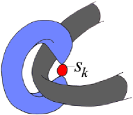
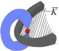
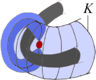
Figure 4: a) Location of a singular qubit (dual, held by a primal defect). b,c) The correlations $\overline{K}$, $K$ affect the $S$-qubit by a Pauli-operator $X$ in (b), and by $Z$ in (c).

6.2 Creating $|\overline{\Psi}_{\text{algo}}\rangle$ among the $S$-qubits

The construction of a topologically protected circuit providing $|\overline{\Psi}_{\text{algo}}\rangle_{S}$ proceeds in three steps. First we show that $|\overline{\Psi}_{\text{algo}}\rangle_{S}$ is local unitarily equivalent to a bi-colorable graph state, by local Hadamard-transformations. Second, we show how to create a bi-colorable graph state. Third, we take care of the Hadamard-transformations.

Equivalence of $|\overline{\Psi}_{\text{algo}}\rangle$ to a bi-colorable graph state.

Denote by $|\Psi\rangle_{{\cal{C}}_{2}}$ the state after the first measurement round ($X$- and $Z$-measurements) in a $QC_{\cal{C}}$-computation on a cluster state $|\phi\rangle_{{\cal{C}}_{2}}$, cf. Section 4. Denote by ${\cal{C}}_{X}$, ${\cal{C}}_{Z}$ the subsets of ${\cal{C}}_{2}\backslash Q$ whose qubits are measured in the $X$- or $Z$-basis, respectively. Further, denote by ${\cal{C}}_{\text{even}}$, ${\cal{C}}_{\text{odd}}$ the sets of even and odd qubits in ${\cal{C}}_{2}$ (checkerboard pattern). The state $|\Psi\rangle_{{\cal{C}}_{2}}$ is given by

$$|\Psi\rangle_{{\cal{C}}_{2}}\sim\left(\bigotimes_{a\in{\cal{C}}_{X}}\frac{I\pm X_{a}}{2}\right)\left(\bigotimes_{b\in{\cal{C}}_{Z}}\frac{I\pm Z_{b}}{2}\right)|\phi\rangle_{{\cal{C}}_{2}}$$ (22)

and has the form $|\Psi\rangle_{{\cal{C}}_{2}}=|\Psi_{\text{algo}}\rangle_{Q}\otimes|\mbox{rest}\rangle_{{\cal{C}}_{2}\backslash Q}$. Further, $|\phi\rangle_{{\cal{C}}_{2}}$ is local unitary equivalent to some CSS-state, $|\phi\rangle_{{\cal{C}}_{2}}=\left(\bigotimes_{i\in{\cal{C}}_{\text{odd}}}H_{i}\right)|CSS\rangle_{{\cal{C}}_{2}}$. Then, with (22) and ${\cal{C}}_{X}^{\prime}:=\left({\cal{C}}_{X}\cap{\cal{C}}_{\text{even}}\right)\cup\left({\cal{C}}_{Z}\cap{\cal{C}}_{\text{odd}}\right)$, ${\cal{C}}_{Z}^{\prime}:=\left({\cal{C}}_{Z}\cap{\cal{C}}_{\text{even}}\right)\cup\left({\cal{C}}_{X}\cap{\cal{C}}_{\text{odd}}\right)$, $|\Psi\rangle_{{\cal{C}}_{2}}\sim\left(\bigotimes_{i\in{\cal{C}}_{\text{odd}}}H_{i}\right)\left(\bigotimes_{a\in{\cal{C}}_{X}^{\prime}}\frac{I\pm X_{a}}{2}\circ\bigotimes_{b\in{\cal{C}}_{Z}^{\prime}}\frac{I\pm Z_{b}}{2}|CSS\rangle_{{\cal{C}}_{2}}\right)=\left(\bigotimes_{i\in{\cal{C}}_{\text{odd}}}H_{i}\right)|CSS^{\prime}\rangle_{{\cal{C}}_{2}}.$ Thus, also the state $|\Psi_{\text{algo}}\rangle$ is l.u. equivalent to a CSS-state,

$$|\Psi_{\text{algo}}\rangle_{Q}=\left(\bigotimes_{q\in{\cal{C}}_{\text{odd}}\cap Q}H_{q}\right)|CSS^{\prime\prime}\rangle_{Q}.$$ (23)

Now, we consider the concatenated-Reed-Muller-encoded resource $|\overline{\Psi}_{\text{algo}}\rangle_{S}$, which may obtained from the bare state $|\Psi_{\text{algo}}\rangle_{Q}$ via encoding, $|\overline{\Psi}_{\text{algo}}\rangle_{S}=\left(\bigotimes_{q\in Q}\mbox{Enc}_{q}\right)|\Psi_{\text{algo}}\rangle_{Q}$. The encoding procedure Enc takes every qubit $q\in Q$ to a set $S(q)$ of qubits, $\bigcup_{q\in Q}S(q)=S$. It has the property that $\mbox{Enc}_{q}\circ H_{q}=\left(\bigotimes_{i\in S(q)}H_{i}\right)\circ\mbox{Enc}^{\prime}_{q}$. Therein, $\mbox{Enc}^{\prime}$ is an encoding procedure for the code conjugated to the Reed-Muller-code, i.e., for the code with the $X$- and the $Z$-block of the stabilizer interchanged. This code is of CSS type, like the Reed-Muller code itself. The encoding procedure changes when passing through the Hadamard-gate because the encoded Hadamard-gate is not local for the Reed-Muller quantum code.

At any rate, the state $|\overline{\Psi}_{\text{algo}}\rangle_{S}$ is l.u. equivalent to a CSS-state encoded with CSS-codes, i.e., to a larger CSS-state, $|\overline{\Psi}_{\text{algo}}\rangle_{S}=\left(\bigotimes_{q\in{\cal{C}}_{\text{odd}}\cap Q}\bigotimes_{i\in S(q)}H_{i}\right)|CSS^{\prime\prime\prime}\rangle_{S}$. Every CSS-state is l.u. equivalent to a bi-colorable graph state [23], by a set of local Hadamard-transformations. Thus, we finally obtain

$$|\overline{\Psi}_{\text{algo}}\rangle_{S}=\bigotimes_{i\in S_{H}}H_{i}\,\,|\Gamma\rangle_{S}.$$ (24)

Therein, $S_{H}$ is some subset of $S$ and $|\Gamma\rangle_{S}$ is a bi-colorable graph state with adjacency matrix of the corresponding graph

$$\Gamma=\left(\begin{array}[]{cc}0&G^{T}\\ G&0\end{array}\right).$$ (25)

Circuit for a bi-colorable graph state.

The circuit layout for the topologically protected creation of an arbitrary bi-colorable graph state is shown in Fig. 5. The circuit consists of a set of horizontal primal and a set vertical dual defects. Each primal defect comes close to each dual defect once, and the two defects may be linked in that region. The form of this junction is decided by a corresponding element of the graph state adjacency matrix $G$. If $G_{i,j}=1$ then the defects are linked and otherwise they are not. In addition, each of the loop defects is linked with an ear-clip shaped defect which holds an $S$-qubit. The graph state in question is formed among these qubits after the remaining qubits have been measured.

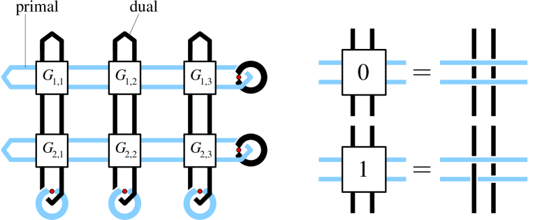
Figure 5: Creation of an arbitrary bi-colorable graph state. The singular qubits are displayed as red circles. $G$ denotes the sub-matrix of the adjacency matrix $\Gamma$ which encodes the edges between primal and dual vertices.

An explanation of the circuit in Fig. 5, for the specific example of a line graph, is given in Fig. 6. From this example it should be clear how the circuit works in general. For the line graph we have the adjacency sub-matrix

$$G_{\text{line}}=\begin{array}[]{cl}\mbox{ }\\ \left(\begin{array}[]{ccc}1&1&0\\ 0&1&1\end{array}\right)&\begin{array}[]{c}b\\ d\end{array}\vspace{2mm}\\ \begin{array}[]{ccc}a&c&e\end{array}\end{array}.$$ (26)

This implies, for example, that in the circuit of Fig. 6a the dual defect winding around the dual $S$-qubit $a$ will be linked with the primal defect winding around the primal $S$-qubit $b$. Now we explain how the stabilizer element $K_{b}=Z_{a}X_{b}Z_{c}$ for the graph state $|\Gamma_{\text{line}}\rangle$ emerges. The other stabilizer generators emerge in the same way.

Consider the relative 2-cycle $c_{2}(b)$ and imagine it being built up step by step. We start around the $S$-qubit $b$. Because $c_{2}(b)$ is primal and $b$ is primal, $K(c_{2}(b))$ affects qubit $b$ by a Pauli-operator $X$, see Eq. (21). Also, $c_{2}(b)$ is bounded by the primal defect encircling $b$.

We move further to the left. At some point, $c_{2}(b)$ approaches a dual defect. Primal correlations cannot end in dual defects. Therefore, $c_{2}(b)$ bulges out and forms a tube wrapping around the dual defect, leading downwards. It ends in the primal defect holding the dual $S$-qubit $c$. $K(c_{2}(b))$ affects qubit $c$ by a Pauli-operator $Z$. Back at the junction, $c_{2}(b)$ continues to expand to the left. It approaches a second dual defect where it forms another tube. In result, the dual $S$-qubit $a$ is affected by a Pauli-operator $Z$. Further to the left, the primal defect closes up and bounds $K(c_{2}(b))$.

$K(c_{2}(b))$ takes the form $X_{b}Z_{a}Z_{c}\bigotimes_{d\in V(b)V}X_{d}$ for some set $V(b)\subset V$. All qubits in $V$ are measured in the $X$-basis (7) such that after these measurements the correlation $K_{b}=\pm Z_{a}X_{b}Z_{c}$ remains. This is a stabilizer generator for the graph state in Fig. 6b since $(a,b)$ and $(c,b)$ are the only edges of the line graph ending in the vertex $b$. For every edge in the graph there is a link among defect loops in the circuit.

a)	b)

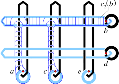
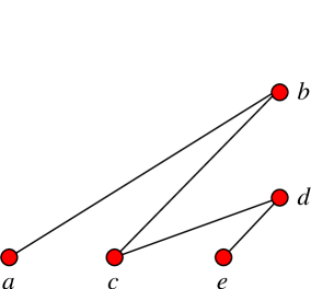
Figure 6: Explanation of the circuit in Fig. 5 for a particular example, the line graph. a) The relative 2-cycle $c_{2}(b)$ which gives rise to the graph-state stabilizer $K_{b}=Z_{a}X_{b}Z_{c}$. b) Graph corresponding to the created graph state.

The proof for the programmable circuit of Fig. 5 realizing a general bi-colorable graph state is similar. As an outline, each stabilizer generator is associated with a doughnut-shaped defect in the circuit. Such a defect bounds a correlation, and this correlation affects one $S$-qubit by $X$. Further, because the considered defect is linked with other defects of the opposite kind, the correlation surface forms tubes. These tubes affect one other $S$-qubit each—the neighbors of the first—by Pauli-operators $Z$.

Implementing the local Hadamard-transformations.

The equivalence between the graph state $|\Gamma\rangle_{S}$ and the encoded algorithm specific resource $|\overline{\Psi}_{\text{algo}}\rangle_{S}$ is by Hadamard-transformations on some subset $S_{H}$ of $S$-qubits. Wherever such a Hadamard-transformation needs to be applied, attach an extra loop to the circuit in Fig. 5,

$$\parbox[c]{170.71652pt}{\psfig{width=165.02606pt}}.$$ (27)

7 Error sources, error correction and fault-tolerance threshold

7.1 Two error models

Below we describe two error models, a simple one and a more realistic one.

Error Model 1.

The cluster state is created only on those cluster qubits which are needed for the computation, i.e., on $V\cup S$. The defect qubits of $D$ are left out.

1. The noise is described by independent partially depolarizing channels acting on each cluster qubit. The noisy state $\rho_{\cal{C}}$ is given by $\displaystyle{\rho_{\cal{C}}=\bigotimes_{a\in{\cal{C}}}T_{a}(p_{1})\,|\phi\rangle_{\cal{C}}\langle\phi|}$, with

   $$T_{a}^{(1)}(p_{1})=(1-p_{1})[I_{a}]+\frac{p_{1}}{3}\left([X_{a}]+[Y_{a}]+[Z_{a}]\right).$$ (28)

2. The classical computation for syndrome processing is instantaneous.

The reason for considering this error model first is its simplicity. We would like to separate the intricacies inherent in the presented error-correction scheme from additional difficulties incurred by a realistic error model. The basic justification for such an approach is this: The error correction used here is topological. Therefore, a threshold should exist regardless of whether independent errors are strictly local or only local in the sense of having a support of bounded size.

The most straightforward method to create a cluster state is from a product state $\bigotimes_{a}|+\rangle_{a}$ via a (constant depth) sequence of $\Lambda(Z)$-gates [10]. If these gates are erroneous, then Error Model 1 does not apply in general. Specifically, one may raise the following objections to Error Model 1:

• No correlated errors are included in Error Model 1. Creating the cluster state via a sequence of gates will, however, lead to correlated errors in the output cluster state.

• Storage errors accumulate in time. There is temporal order among the measurements such that the computation takes a certain time $t_{\text{comp}}$ which cannot be bounded by a constant for all possible computations. As a consequence, for the qubits measured in the final round the local noise rate increases monotonically with $t_{\text{comp}}$ and exceeds the error threshold.

• To leave the $D$-qubits out is a deviation from the originally envisioned setting: the cluster state on $S\cup V$ is algorithm-specific.

To account for these inadequacies, we consider a second error model.

Error Model 2.

A cluster state on a bcc-symmetric lattice is created in four steps of nearest-neighbor $\Lambda(Z)$-gates. The gate sequence is as shown in Fig. 7. Errors occur due to the erroneous preparation of the initial $|+\rangle$-qubits, erroneous $\Lambda(Z)$-gates in the process of creating the cluster state, storage and measurement.

1. The computation is split up into steps which performed on sub-clusters ${\cal{C}}_{k}$. In each step, unmeasured qubits remaining from the previous step—the hand-over qubits—are loaded into a cluster state on a sub-cluster. Subsequently, all but a few cluster qubits (the new hand-over qubits) are measured. The steps have their temporal depth adjusted such that each qubit, after being locally prepared and entangled, waits at most a constant number $t_{0}$ of time steps until its measurement occurs, $t_{0}\geq 1$. Error in storage is described by a partially depolarizing noise with error probability $p_{S}$ per time step.

2. The erroneous preparation of initial $|+\rangle$-qubits is modeled by the perfect procedure followed by local depolarizing noise (28), with probability $p_{P}$. Measurement is described by perfect measurement preceded by partially depolarizing noise with error probability $p_{M}$. The erroneous $\Lambda(Z)$-gates are modeled by the perfect gate followed by a 2-qubit depolarizing channel

   $$T^{(2)}_{e,f}(p_{2})=(1-p_{2})[I_{e,f}]+\frac{p_{2}}{15}\left([I_{e}\otimes X_{f}]+...+[Z_{e}\otimes Z_{f}]\right).$$ (29)

3. Classical syndrome processing is instantaneous.

In the subsequent sections we compute a fault-tolerance threshold for both error models. In Error Model 2, storage error will cause the minimum damage for the smallest possible value of $t_{0}$, which is $t_{0}=1$. In this case, each sub-cluster carries a subset of $S$-qubits with no mutual temporal dependence. All qubits in $V$ and $D$, except the hand-over qubits (See Appendix A), are measured immediately after being entangled. The measurement of the $S$-qubits has to wait one time step. Henceforth we set $t_{0}=1$.

Figure 7: Steps of $\Lambda(Z)$-gates for the creation of a cluster state on a bcc-symmetric lattice, for the sub-clusters ${\cal{C}}_{k}$. For $k$ odd, the sequence is $1\rightarrow 2\rightarrow 3\rightarrow 4$, and for $k$ even it is $3\rightarrow 4\rightarrow 1\rightarrow 2$.

7.2 Methods for error correction and the threshold value

There are different methods of error correction associated with the different regions $V$, $S$ and $D$ of the cluster. In $D$, there are as many inequivalent errors as there are syndrome bits, such that the error correction is trivial. The error correction in $V$ is based on the random plaquette $\mathbb{Z}_{2}$-gauge model in three dimensions [18]. The error correction in $S$ is carried out using the (concatenated) quantum Reed-Muller code.

Error correction in $D$.

In the domain $D(d)$ of the defect only $Z$-errors matter for face qubits and only $X$-errors matter for edge qubits. Any other errors may be absorbed into the subsequent measurements (7). The $X$-errors on edges may be relocated to $Z$ errors on the neighboring face qubits via $X_{e}\cong K_{e}X_{e}$, such that we need to consider $Z$-errors on face qubits only. For each face in $d$ we learn one syndrome bit, yielding a unique syndrome for each error configuration.

However, if an error $X_{e}$ on an edge qubit $e$ in the surface of defect $d$ is relocated, the equivalent error $K_{e}X_{e}$ may partially be outside $D(d)$. After error correction in $D(d)$, an individual $Z$-error on a face qubit in $V$ is left next to $D(d)$. This affects the error correction in $V$ near $D$; see below.

Error correction in $V$.

First consider a scenario where the entire cluster consists of the region $V$ (i.e., there are no defects and no singular qubits). Error correction on the primal lattice ${\cal{L}}$ and the dual lattice $\overline{\cal{L}}$ run separately. Here we consider error correction on the primal lattice only; error correction on the dual lattice is analogous.

The error chains live on the edges of the lattice ${\cal{L}}$ and leave a syndrome at the end points, which are vertices of ${\cal{L}}$. This is exactly the scenario which has been considered for topological quantum memory in [18], and subsequently the results of [18] that we need in the present context are briefly summarized. The connection between topological error correction and cluster states has been made in [14] for the purpose of creating long-range entanglement in the presence of noise.

Given a particular syndrome and an error chain $E(c_{1})$ compatible with this syndrome, we are interested in the total probability $P(c_{1})$ of the homology class of $c_{1}$,

$$P(c_{1})=\sum_{z_{1}\in Z_{1}}p(c_{1}+z_{1}),$$ (30)

where $p(c_{1}^{\prime})$ is the probability of an individual error chain $E(c_{1}^{\prime})$, and the sum is over all 1-cycles. For error correction we infer that the physical error which occurred was from the homology class with the largest probability.

If the errors on the lattice edges occur independently with a probability $q$ then the problem of computing $P(c_{1})$ for a given chain $c_{1}$ can be mapped onto a problem from statistical mechanics, namely the random plaquette $\mathbb{Z}_{2}$-gauge model in three dimensions [18]. The crossover from high fidelity error correction at small error rates to low fidelity error correction at high error rates corresponds to a phase transition in this model. A numerical estimate of the critical error rate is $q_{\text{c}}=0.033\pm 0.001\;$[25].

As far as is known, the classical operational resources required to find the most likely error homology class consistent with a given syndrome scales exponentially in the number of error locations. The assumption of the classical processing being instantaneous cannot be justified under these conditions. However, it is possible to trade threshold value for efficiency in the error correction procedure. A reasonable approximation to the maximum probability for a homology class of errors is the probability of the lowest weight admissible chain. The minimum-weight perfect matching algorithm [26, 27] computes this chain using only polynomial operational resources. A numerical estimate to the threshold with this algorithm for error correction is $q^{\prime}_{\text{c}}=0.0293\pm 0.0002$ [28].

Remark: The topological error threshold is estimated in numerical simulations of finite-size systems. For this purpose, the probability of logical error is plotted vs. the physical error parameter for various system sizes. For sufficiently large lattices (such that finite-size effects are small), we expect these curves to follow a universal scaling ansatz near the threshold such that they share a common intersection point and their slopes are proportional to a common power of the lattice size. As the system size is increased to infinity, we then expect the curves to approach a step function which transitions at the threshold value of the physical error parameter.

The above quoted threshold value is for independent errors on the edges of ${\cal{L}}$. Do the models for the physical error sources of Section 7.1 lead to such independent errors? The answer is ‘yes’ for error Model 1 and ‘no’ for error Model 2. For the latter, we need to consider a modified RPGM with correlated errors among next-to-nearest neighbors. Specifically, for Error Model 1 the relation between the local rate $p_{1}$ of the physical depolarizing error and the error parameter $q$ that shows up in the RPGM is

$$q=\frac{2}{3}p_{1},\;\;\;\;\;\;\;\;\text{for Error Model 1}.$$ (31)

Given a threshold of $q=2.93\%$ [28] for error correction via the minimum weight perfect matching algorithm in the bulk, then the corresponding depolarizing error rate that can be tolerated is

$$p_{1,\text{c}}=4.4\times 10^{-2},\;\;\;\;\mbox{(in $V$)}.$$ (32)

Figure 8: Threshold estimation in lattices of finite size, for periodic boundary conditions. Here, with $\Lambda(Z)$-gates as the only error source, we find a threshold of $p_{2,\text{c}}=9.6\times 10^{-3}$. In the inset, best fits to the universal scaling ansatz are drawn. Error bars denote two standard deviations due to finite sampling size.

For Error Model 2, first consider the case where only the $\Lambda(Z)$-gates are erroneous, $p_{P}=p_{S}=p_{M}=0$. Then, in addition to local errors with a rate $q_{1}$ there exist correlated errors with error rate $q_{2}$ for each pair of opposite edges in all faces of ${\cal{L}}$. That is, with a probability $q_{2}$ simultaneous errors are introduced on opposite edges of the faces in ${\cal{L}}$. The local noise specified by $q_{1}$ and the two-local noise specified by $q_{2}$ are independent processes. The relations between the error parameter $p_{2}$ of the $\Lambda(Z)$-gates and the parameters $q_{1},q_{2}$ of the RPGM with correlated errors are

$$\begin{array}[]{rcl}q_{1}&=&\displaystyle{\frac{32}{15}p_{2}\left(1-\frac{8}{15}p_{2}\right)\left(\frac{64}{225}p_{2}^{\,\,2}+\left(1-\frac{8}{15}p_{2}\right)^{2}\right),}\\ q_{2}&=&\displaystyle{\frac{1}{2}-\sqrt{\frac{1}{4}-\frac{4}{15}p_{2}}\,=\,\frac{4}{15}p_{2}+O(p_{2}^{\,\,2}).}\end{array}$$ (33)

The correlation of errors on sites separated by a distance of two arises through error propagation in the creation of the cluster state. Correlations among errors on next-neighboring sites play no role because such errors live on different lattices (${\cal{L}}$ and $\overline{\cal{L}}$) and are corrected independently.

The only effect of $p_{P},p_{S},p_{M}>0$ is an enhanced local error rate $q_{1}$. We give the relations to leading order only; they read

$$\begin{array}[]{rcl}q_{1}&=&\displaystyle{\frac{32}{15}p_{2}+\frac{2}{3}\left(p_{P}+p_{S}+p_{M}\right),\vspace{1mm}}\\ q_{2}&=&\displaystyle{\frac{4}{15}p_{2},}\end{array}\;\;\;\;\;\;\;\;\;\;\;\text{for error Model 2}.$$ (34)

See Fig. 8 for a simulation of error correction under faulty $\Lambda(Z)$-gates as the only error source, which gives rise to correlated noise between neighboring edge qubits. If we define $x=(p_{2}-p_{2,c})L^{1/\nu_{0}}$ then the universal scaling ansatz states that fidelity $F$ should be a function dependent only on the scaling parameter $x$ in the vicinity of the threshold [28]. We find very good agreement (with $R^{2}>.9991$) for $F=A+Bx+Cx^{2}$, where we fit for constants $A$, $B$, $C$, $p_{2,c}$, and $\nu_{0}$. This gives very tight bounds on the critical probability $p_{2,c}=9.6\times 10^{-3}$. Interestingly, we also find $\nu_{0}=1.00\pm 0.02$, which indicates that this model belongs to the same universality class as the purely local error model of the 3D-RPGM [28].

In Fig. 9 the threshold trade-off curve between $p_{P}+p_{S}+p_{M}$ and $p_{2}$ is displayed. Numerically, we obtain for the thresholds in the bulk

$$\begin{array}[]{rclcl}p_{P}=p_{S}=p_{M}&=&1.46\times 10^{-2},&&\mbox{for }p_{2}=0,\\ p_{2}&=&0.96\times 10^{-2},&&\mbox{for }p_{P}=p_{S}=p_{M}=0,\\ p_{i}&=&0.58\times 10^{-2},&&\mbox{for }p_{P}=p_{S}=p_{M}=p_{2}.\end{array}$$ (35)

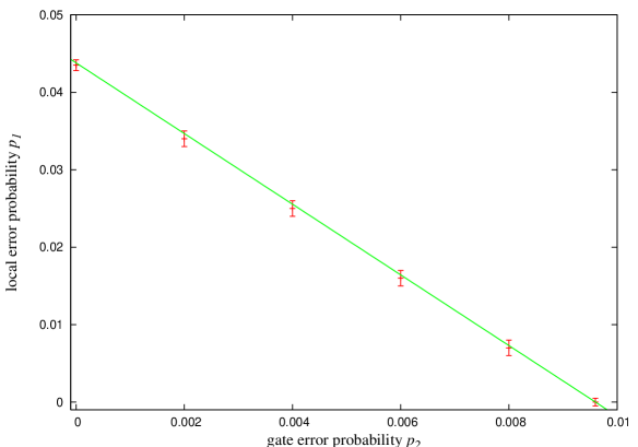
Figure 9: Trade-off curve for the threshold value in the presence of local and two-local errors. Horizontal axis: two-qubit gate error $p_{2}$, vertical axis: local error rate $p_{P}+p_{S}+p_{M}$.

Error correction in $V$ near $D$.

In the presence of defects there are two modifications to error processes in $V$. First, the length scale for the minimum extension of a non-trivial error cycle shrinks. Second, there is a surface effect; the effective error rate for qubits in $V$ next to the surface of defects is enhanced by a constant factor.

1. Length scale for non-trivial errors: For comparison, consider a cluster cube of finite size $2L\times 2L\times 2L$. A non-trivial error cycle must stretch across the entire cube and thus has a weight of at least $L$. The lowest weight errors which are misinterpreted by the error correction procedure occur with a probability $q^{L/2}$. The total error probability incurred by such errors may therefore be expected to decrease exponentially fast in $L$, which is confirmed in numerical simulations [14].

In the presence of defects, the dominant sources for logical error are 1-chains that either wind around a defect or that begin and end in a defect and intersect a correlation surface (2-chain) in between; see Fig. 10. The relevant length scales are thus the thickness (circumference) and the diameter of the defects. They are much smaller than $L$.

Specifically, consider a defect with circumference $u$ and length $l$ which bounds a correlation surface $c_{2}$, such that $|\{\partial c_{2}\}|=l$. An error cycle winding around the defect has a weight of at least $u+8\approx u$, and there are $l$ such minimum weight cycles. Therefore, the probability $p_{E}(u,l)$ for affecting $K(c_{2})$ by an error is, to lowest contributing order,

$$p_{E}(u,l)=l\frac{u!}{(u/2)!^{2}}q^{u/2}\approx l\exp\left(\frac{\ln 4q}{2}u\right)\frac{1}{\sqrt{\pi/2\,u}}.$$ (36)

In the range of validity for the above expansion in powers of $q$, the error is still exponentially suppressed in the relevant length scale $u$.

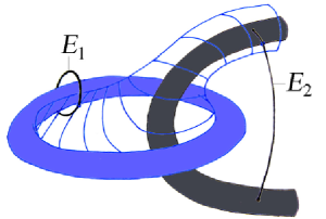
Figure 10: Sources for logical error in the presence of defects.

2. Surface effects: As discussed above, the error level is enhanced for qubits in $V$ near the surface of a defect. If the defect is primal (dual), the enhancement occurs on dual (primal) qubits. This effect will—if anything—lower the threshold. But there is another effect: the presence of the defect changes the boundary conditions. In case of a primal defect, the boundary conditions on the defect surface become rough for the primal lattice and smooth for the dual lattice. Dual error chains cannot end in a primal defect, as we noted earlier. For the dual lattice, there is excess syndrome available at the defect surface. This effect will—if anything—increase the threshold. Our intuition is that neither effect has an impact on the threshold value. The threshold should, if the perturbations at the boundary are not too strong, still be set by the bulk.

We have performed numerical simulations for lattices of size $L\times L\times 2L$, where half of the lattice belongs to $V$ and the other half to the defect region $D$. The error rate is doubled near the mutual boundary of the regions and there is no remaining error in $D$. Simulations are feasible with reasonable effort up to $L\approx 20$. We find that finite-size effects (due to the smooth boundary conditions) are still noticeable up to these lattice sizes, but the intersection point of fidelity curves for nearby lattice sizes is slowly converging to a threshold value around that of the bulk ($\sim 2.9\%$).

a)		b)

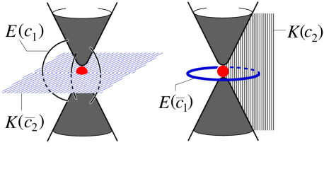
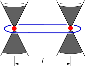
Figure 11: Topological error correction in the presence of defects. a) Short error cycles intersect with the correlation surfaces and thereby jeopardize the topological error correction. b) Correlated errors on $S$-qubits are suppressed exponentially in the qubit separation $l$.

Error correction in $V$ near a junction between $D$ and $S$.

Near an $S$-qubit there exist relative error cycles of small length, see Fig. 11a, and the topological error correction breaks down. As a result, the effective error on an $S$-qubit is enhanced by its surrounding. To compute the effective error probabilities, we replace every low-weight error-chain $E(\gamma)$ that results in a logical error after error correction by an equivalent error $E_{S}(\gamma)$ acting on the $S$-qubits. The error correction converts $E(\gamma)$ into $E(c_{1}(\gamma))$ with $c_{1}(\gamma)$ a relative 1-cycle. ‘Equivalent’ means that $E(c_{1}(\gamma))$ and $E_{S}(\gamma)$ act in the same way on the stabilizer generators $\{K_{\overline{\Psi},s}|\;s\in S\}$ of the induced state $|\overline{\Psi}_{\text{algo}}\rangle_{S}$, i.e., $[E(c_{1}(\gamma))E_{S}(\gamma),K_{\overline{\Psi},s}]=0$ for all $s\in S$. The relevant correlations to check are $K(\overline{c}_{2})$ and $K(c_{2})$ displayed in Fig. 11a.

It is important to note that the effective error on the $S$-qubits is local. This arises because only error chains causing a 1-qubit error may have small length. Error chains causing a correlated error on the $S$-qubits are suppressed exponentially in the qubit separation. See Fig. 11b.

We compute the effective error channel on the $S$-qubit to first order in the error probabilities only. For error Model 1 the error enhancement only affects sub-leading orders of $p_{1}$,

$$T^{(1)}_{s}=(1-p_{1})[I_{s}]+\frac{p_{1}}{3}\left([X_{s}]+[Y_{s}]+[Z_{s}]\right).$$ (37)

For Error Model 2 the effective error channel on an $S$-qubit is not universal but depends on the precise shape of the defect double-tip near the $S$-qubit. For our calculation we use the defect shape displayed in Fig. 12. The defect is one-dimensional nearest to the $S$-qubit, and farther away becomes three-dimensional. The effective error channel then is

$$\begin{array}[]{rcl}\tilde{T}^{(1)}_{s}&=&\displaystyle{\left(1-\frac{2}{3}p_{P}-\frac{7}{3}p_{S}-\frac{7}{3}p_{M}-\frac{94}{15}p_{2}\right)[I_{s}]\,+\left(2p_{2}+\frac{5}{3}p_{S}+\frac{5}{3}p_{M}\right)[X_{s}]\,+}\\ &&\displaystyle{+\left(\frac{2}{5}p_{2}+\frac{1}{3}p_{S}+\frac{1}{3}p_{M}\right)\,[Y_{s}]+\left(\frac{2}{3}p_{P}+\frac{1}{3}p_{S}+\frac{1}{3}p_{M}+\frac{58}{15}p_{2}\right)[Z_{s}]}.\end{array}$$ (38)

The individual contributions to (38) are listed in Appendix B.

a)	b)

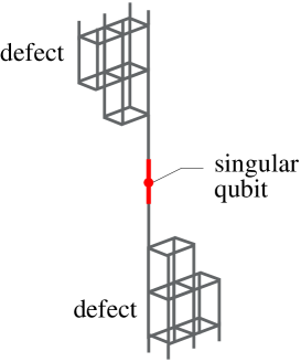
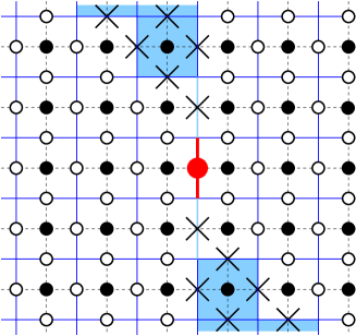
Figure 12: Shape of the defect near an $S$-qubit (red). a) Three-dimensional view. b) Cross-section through the cluster. Edges which belong to the defect are marked as “$\times$”. Black dashed lines connect neighbors on the cluster. Blue underlay: faces in the defect. Even/odd qubits: $\bullet/\circ$.

Error correction in $S$.

The $S$-qubits are protected by the concatenated Reed-Muller code. This code corrects for the errors (37)/(38) that remain after error correction in $V$ and $D$.

The $S$-qubits are all measured in the eigenbases of $\frac{X\pm Y}{\sqrt{2}}$. Then, an $X$- or a $Y$-error is equivalent to a $Z$-error with half the probability. This is easily verified for the case where $X$- and $Y$-errors occur with the same probability. W.l.o.g. assume the measurement basis is $\frac{X+Y}{\sqrt{2}}$. Then $[X]+[Y]=\frac{[X+Y]}{\sqrt{2}}+\frac{[X-Y]}{\sqrt{2}}=\frac{[X+Y]}{\sqrt{2}}([I]+[Z])\cong[Z]$. But the statement is, to leading and next-to-leading order in the error probability, also true when $X$- and $Y$-errors do not occur with equal probability; see Appendix C. We may thus convert the $X$- and $Y$-errors in (37) and (38) into $Z$-errors. The corresponding error probability $p_{Z}$ is

$$\begin{array}[]{rclcl}p_{Z}&=&\displaystyle{\frac{2}{3}{p_{1}}},&&\mbox{for error Model 1},\vspace{1mm}\\ p_{Z}&=&\displaystyle{\frac{76}{15}p_{2}+\frac{2}{3}p_{P}+\frac{4}{3}p_{M}+\frac{4}{3}p_{S},}&&\mbox{for error Model 2}.\end{array}$$ (39)

The fault-tolerance threshold of the concatenated $[15,1,3]$-Reed-Muller code for independent $Z$-errors with probability $p_{Z}$ is $1.09\times 10^{-2}$. As we discuss all Reed-Muller error correction to leading order only, we take the leading order estimate

$$p_{Z,\text{c}}=\frac{1}{105}\approx 0.95\times 10^{-2}.$$ (40)

For Error Model 1, from (39) and (40) we obtain the threshold

$$p_{1,\text{c}}=\frac{1}{70}\approx 1.4\times 10^{-2},\;\;\;\;\;\;\mbox{(in $S$)}.$$ (41)

For error Model 2 we obtain

$$\begin{array}[]{rclcl}p_{P,\text{c}}=p_{S,\text{c}}=p_{M,\text{c}}&=&\displaystyle{\frac{1}{350}\approx 0.29\times 10^{-2}},&&\mbox{for }p_{2}=0,\vspace{1mm}\\ p_{2,\text{c}}&=&\displaystyle{\frac{1}{532}\approx 0.19\times 10^{-2}},&&\mbox{for }p_{P}=p_{S}=p_{M}=0,\vspace{1mm}\\ p_{i,\text{c}}&=&\displaystyle{\frac{1}{882}\approx 0.11\times 10^{-2}},&&\mbox{for }p_{P}=p_{S}=p_{M}=p_{2},\end{array}\;\;\;\;\;\;\;\;\mbox{(in $S$)}.$$ (42)

The topological error correction in $V$ and the Reed-Muller error correction in $S$ run separately, and all that remains is to check which mechanism breaks down first. By comparison of Equation (32) with (41) and Equation (35) with (42), we find for both error models that the Reed-Muller error correction collapses first. It therefore sets the overall threshold. In Error Model 1, the critical error probability for local depolarizing error is $1.4\times 10^{-2}$. In Error Model 2, for the case where preparation, gate, storage and measurement errors each have equal strength, the error threshold for the individual processes is $1.1\times 10^{-3}$.

8 Overhead

Denote by $N$ the number of qubits in the algorithm-specific resource state $|\Psi_{\text{algo}}\rangle_{Q}$. $N$ is also the number of non-Clifford one-qubit rotations in a quantum circuit realizing the algorithm “algo”. What is the number $N_{\text{ft}}$ of cluster qubits required to perform the same computation fault-tolerantly?

The qubit overhead factor for Reed-Muller error correction is

$$O_{\text{RM}}=\left(\frac{\log N}{\log p_{\text{c}}/p}\right)^{\gamma},$$ (43)

where $\gamma=\log_{2}15\approx 3.91$, and $p$ is the actual and $p_{\text{c}}$ the critical Reed-Muller error rate. The set $S$ consists of $|S|=NO_{\text{RM}}$ qubits.

We need to determine the additional overhead due to topological error correction. We choose a separation $r$ between strands of a defect loop, and a strand diameter of $r/2$.

The dimensions of the cluster thus are $\mbox{width},\mbox{depth}\leq 3/2\,rNO_{\text{RM}}$, $\mbox{height}=4r$. The most likely errors then occur with a probability of $\exp(-\kappa(p)r)$, (36), and there are less than $3r(NO_{\text{RM}})^{2}$ locations for them (primal+dual). We require that $3r(NO_{\text{RM}})^{2}\exp(-\kappa(p)r)\approx 1$, such that in the large $N$ limit

$$r\approx\frac{2}{\kappa(p)}\ln N.$$ (44)

Double-logarithmic corrections are omitted. The total number of qubits is given by $N_{\text{ft}}=\mbox{width}\times\mbox{depth}\times\mbox{height}\leq 9r^{3}(NO_{\text{RM}})^{2}$, such that

$$N_{\text{ft}}\sim N^{2}\left(\log N\right)^{3+2\gamma}.$$ (45)

The overhead is polynomial. The values of the exponents in the above expression may be reduced in more resourceful adaptations of the presented scheme.

9 Discussion

We have described a scheme for fault-tolerant cluster state universal quantum computation which employs topological error correction. This is possible because of a link between cluster states and surface codes. In addition to the topological method, we make use of a Reed-Muller quantum code which ensures that non-Clifford operations can be performed fault-tolerantly by local measurements.

The error threshold is $1.4\%$ for an ad-hoc error model with local depolarizing error and $0.11\%$ for a more detailed error model with preparation-, gate-, storage- and measurement errors. We have not tried to optimize for either threshold value or overhead here; the foremost purpose of this paper is to explain the techniques. With regard to a high threshold, the obvious bottleneck is the Reed-Muller code. The error threshold imposed by this code on the cluster region $S$ is—depending on the error model—a factor of 3 to 5 times worse than the threshold obtained from the topological error correction in $V$. To increase the threshold one may replace this code by another CSS code with property (5) that has a higher error threshold, provided such a code exists. Alternatively, one may probe the Reed-Muller code in error detection, as in magic state distillation [17]. The error detection threshold is $14\%$, which indicates that there is some room for improvement.

Part of the investigations in this paper are numerical simulations, and we would like to comment on their impact on the threshold value. Numerics are encapsulated only in the threshold estimate for topological error correction which is much higher than the overall threshold. Our final threshold estimate stems from the Reed-Muller code and is analytical.

Acknowledgments:

We would like to thank Sergey Bravyi, Frank Verstraete, Alex McCauley, Hans Briegel and John Preskill for discussions. JH is supported by ARDA under an Intelligence Community Postdoctoral Fellowship. KG is supported by DOE Grant No. DE-FG03-92-ER40701. RR is supported by MURI under Grant No. DAAD19-00-1-0374 and by the National Science Foundation under contract number PHY-0456720. Additional support was provided by the Austrian Academy of Sciences.

The appendices are relevant for Error Model 2 only.

Appendix A Connecting sub-clusters

The cluster ${\cal{C}}$ consists of a set of sub-clusters ${\cal{C}}_{k}$, ${\cal{C}}=\bigcup_{k}{\cal{C}}_{k}$ which are prepared in sequence. Two successive sub-clusters ${\cal{C}}_{k}$, ${\cal{C}}_{k+1}$ have an overlap, ${\cal{C}}_{k}\cap{\cal{C}}_{k+1}=H_{k}\subset V\cup D$. $H_{k}$ is a set of locations for hand-over qubits. Each graph edge (corresponding to a $\Lambda(Z)$-gate in cluster state creation) can be unambiguously assigned to one sub-cluster. The set of edges ending in one vertex either belongs to one or to two sub-clusters. In the latter case, the vertex is the location for a hand-over qubit.

If $k$ is odd, the cluster state creation procedure on ${\cal{C}}_{k}$ is the sequence $1\rightarrow 2\rightarrow 3\rightarrow 4$. If $k$ is even, the sequence is $3\rightarrow 4\rightarrow 1\rightarrow 2$. As shown in Fig. 13b, connecting the sub-clusters proceeds smoothly. Consider, for example, the sub-cluster ${\cal{C}}_{1}$. With the exception of a subset of the hand-over qubits to ${\cal{C}}_{2}$, the qubits in ${\cal{C}}_{1}$ are prepared at $t=0$, entangled in steps 1 to 4, and measured at $t=5,6$. Specifically, the $V$- and $D$-qubits are measured at time $t=5$, while the $S$-qubits are measured at time $t=6$ with measurement bases adapted according to previous measurement outcomes. The sub-clusters ${\cal{C}}_{k}$ are chosen such that there is no temporal order among the measurements on qubits within $S\cap{\cal{C}}_{k}$, for all $k$. Then, the $S$-qubits wait for one time step in which a storage error may occur.

a)	b)

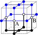
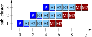
Figure 13: Connecting sub-clusters. a) Elementary cell of ${\cal{L}}$. The old sub-cluster is displayed in blue, the new in black; “$\circ$”; hand-over qubits, “$\bullet$”: qubits within one sub-cluster. b) Temporal order of operations. “P”: $|+\rangle$-preparation, “E1-E4”: steps of parallel $\Lambda(Z)$-gates, M1, M2: measurement.

The hand-over qubits stay in the computation no longer than the other $V$- and $D$-qubits. They form two subsets, $H_{1}=A\cup B$; see Fig. 13a. The qubits in $A$ are prepared at $t=0$, entangled in time steps 1 to 4 and measured in at $t=5$. They cause no change in the error model.

The qubits in $B$ are not acted upon by a gate until time step 2 (since the potential interaction partner of step 1 isn’t there yet), so they are prepared at time $t=1$. The final interaction involving the $B$-qubits is in step 5, and they are measured in step 6. Between preparation and measurement, the $B$-qubits are in the computation for four time steps in each of which they are acted upon by a gate. No additional storage error occurs. There is one modification due to the $B$-qubits. The temporal order of $\Lambda(Z)$-gates involving the qubits $b\in B$ is changed. As a result, the correlated errors on the edge qubits of the faces $\{c_{2}\}=b$ are not among pairs of opposite edge qubits but among pairs of neighboring edge qubits. So, the error rates $q_{1}$ and $q_{2}$ in (34) are unchanged, but $q_{2}$ characterizes a slightly different process.

We expect this to be a minor effect. The overall threshold is still set by the threshold for Reed-Muller error-correction, which is some five times smaller than the simulated threshold for topological error correction.

Appendix B Effective error channel on the $S$-qubits

The effective error on an $S$-qubit stems from the $S$-qubit itself and its immediate surrounding shown in Fig. 14 and from the two edge-qubits in the one-dimensional section of the defect, which are not protected by any syndrome. Of the latter each contributes an error

$$E_{\text{defect}}=\left(\frac{4}{5}p_{2}+\frac{2}{3}p_{S}+\frac{2}{3}p_{M}\right)[X_{s}].$$ (46)

The preparation error does not contribute, because the corresponding $Z$-error on the defect qubit is absorbed in the $Z$-measurement.

The effective error of the center qubit $s\in S$ stems from operations that act on $s$ directly, from $X$- or $Y$-errors propagated to $s$ by the $\Lambda(Z)$-gates and from short nontrivial cycles. Specifically, there are four non-trivial cycles of length 3. One of them is denoted as $E(c_{1})$ in Fig. 14. Because of the correlations in the forward-propagated errors these cycles have weight 2 and cause inconclusive syndrome at lowest order in the error probability. There are further error cycles of length 3, such as $E(c_{1}^{\prime})$ in Fig 14. But they have weight 3 even for Error Model 2 and do not contribute to the lowest order error channel. We perform a count including all error sources in the cluster region displayed in Fig. 14, right. There is one convention that enters into the count. Namely, the error $Z_{a}Z_{b}Z_{c}Z_{d}$ (see Fig. 14) is a non-trivial error cycle such that the errors $Z_{a}Z_{b}$ and $Z_{c}Z_{d}$ have the same weight and the same syndrome but different effect on the computation, $X_{s}$ vs. $I_{s}$. When the corresponding syndrome occurs, we assert that a logical $X$-error occurred and correct for it. We obtain

$$E_{\text{central}}=\left(\frac{2}{5}p_{2}+\frac{1}{3}p_{S}+\frac{1}{3}p_{M}\right)\left([X_{s}]+[Y_{s}]\right)+\left(\frac{2}{3}p_{P}+\frac{1}{3}p_{S}+\frac{1}{3}p_{M}+\frac{58}{15}p_{2}\right)[Z_{s}].$$ (47)

The sources (46) and (47) combined, $E_{\text{central}}+2\times E_{\text{defect}}$, lead to the local error channel (38).

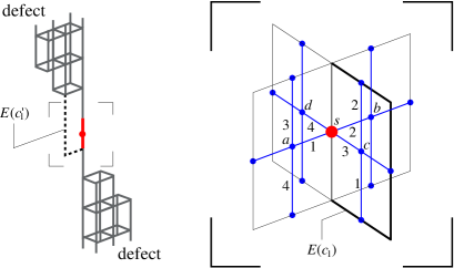
Figure 14: Lattice around an $S$-qubit. Left: Location of the $S$-qubit (red) and the defect (gray). $E(c_{1}^{\prime})$ is an error cycle of length 3 and weight 3 for Error Models 1 and 2. Right: Detail. $E(c_{1})$ is a non-trivial error cycle of length 3 which has weight 2 in error Model 2. Red: $S$-qubit, black: lattice ${\cal{L}}$ for topological error correction. The cluster edges (blue) correspond to $\Lambda(Z)$-gates whose temporal order is as indicated.

Appendix C Conversion of $X$- and $Y$-errors on $S$-qubits

Here we show that an $X$- or $Y$-error on an individual $S$-qubit $s$ with probability $p$ is equivalent to a $Z$-error on that qubit with probability $p/2$, $p[X_{s}]\cong p[Y_{S}]\cong p/2\,[Z_{s}]$. The qubit $s$ may be measured in the eigenbasis of $\frac{X+Y}{\sqrt{2}}$ or of $\frac{X-Y}{\sqrt{2}}$. W.l.o.g. assume the qubit $s$ is measured in the eigenbasis of $\frac{X+Y}{\sqrt{2}}$. Then, $X_{s}=\frac{X_{s}+Y_{s}}{\sqrt{2}}\frac{I_{s}-iZ_{s}}{\sqrt{2}}\cong\frac{I_{s}-iZ_{s}}{\sqrt{2}}$. The $X$-error is equivalent to a coherent $Z$-error and we need to check whether the coherences matter. More generally, for the described scenario with the subsequent measurement a probabilistic local error channel $(1-p_{X}-p_{Y}-p_{Z})[I_{s}]+p_{X}[X_{s}]+p_{Y}[Y_{s}]+p_{Z}[Z_{s}]$ is equivalent to a channel with coherent errors

$$\rho\longrightarrow(1-q)\rho+qZ_{s}\rho Z_{s}+i\tilde{q}\left(\rho Z_{s}-Z_{s}\rho\right),$$ (48)

with

$$q=p_{Z}+\frac{p_{X}+p_{Y}}{2},\;\;\;\tilde{q}=\frac{p_{X}-p_{Y}}{2}.$$ (49)

Now assume that all $S$-qubits are affected individually by the error channel (48). The Reed-Muller error correction at successive levels maps these channels to channels of the same form, one coding level higher up. The parameters $q_{l}$, $\tilde{q_{l}}$ at coding level $l$ obey recursion relations which, up to fourth order, read

$$\begin{array}[]{lcl}q_{l+1}&=&\displaystyle{105\,q_{l}^{2}\,(1-q_{l})^{13}+35\,q_{l}^{3}\,(1-q_{l})^{12}+1260\,q_{l}^{4}\,(1-q_{l})^{11}+630\,\tilde{q}_{l}^{4}\,(1-q_{l})^{11}},\vspace{1mm}\\ \tilde{q}_{l+1}&=&\displaystyle{70\,\tilde{q}_{l}^{3}\,(1-q_{l})^{12}-1680\,\tilde{q}_{l}^{3}q_{l}\,(1-q_{l})^{11}}.\end{array}$$ (50)

If we compare (50) to the recursion relation of $q$ for probabilistic $Z$-error, a deviation first shows up at fourth order. The discussion of Reed-Muller error correction in this paper is confined to leading order. The leading order result for the threshold, $q_{\text{c}}=1/105$, is not affected by the coherences in the error (48). Probabilistic $X$-and $Y$-errors influence the threshold by contributing half their weight to the probability of an effective $Z$-error; see (49).

References

- [1] E. Knill, R. Laflamme, W.H. Zurek, Proc. Roy. Soc. London A 454, 365 (1998).
- [2] D. Aharonov and M. Ben-Or, Proc. 29th Ann. ACM Symp. on Theory of Computing, 176 (New York, ACM, 1998); D. Aharonov, M. Ben-Or, quant-ph/9906129 (1999).
- [3] D. Gottesman, PhD thesis, Caltech (1997), quant-ph/9705052.
- [4] P. Aliferis, D. Gottesman, J. Preskill, quant-ph/0504218.
- [5] E. Knill, Nature 434, 39 (2005).
- [6] A. Kitaev, Ann. Phys. 303, 2 (2003); quant-ph/9707021.
- [7] J. Preskill, quant-ph/9712048.
- [8] C. Mochon, Phys. Rev. A 67, 022315 (2003).
- [9] R. Raussendorf and H.-J. Briegel, Phys. Rev. Lett. 86, 5188, (2001).
- [10] H.-J. Briegel and R. Raussendorf, Phys. Rev. Lett. 86, 910, (2001).
- [11] R. Raussendorf, PhD thesis, University of Munich (2003).
- [12] M.A. Nielsen, C.M. Dawson, Phys. Rev. A 71, 052312 (2005); C.M. Dawson, H.L. Haselgrove, and M.A. Nielsen, quant-ph/0509060.
- [13] P. Aliferis, D. Leung, quant-ph/0503130.
- [14] R. Raussendorf, S. Bravyi, J. Harrington, Phys. Rev. A 71, 062313 (2005).
- [15] S. Bravyi and A. Kitaev, quant-ph/980092.
- [16] E. Knill, R. Laflamme, W. Zurek, quant-ph/9610011.
- [17] S. Bravyi and A. Kitaev, Phys. Rev. A 71, 022316 (2005).
- [18] E. Dennis, A. Kitaev, A. Landahl and J. Preskill, quant-ph/0110143.
- [19] F.J. MacWilliams, N.J.A. Sloane, The Theory of Error-Correcting Codes, North-Holland Publishing Company, Amsterdam (1977).
- [20] J.W. Vick, Homology theory: an introduction to algebraic topology, Springer, New York (1994), originally published: Academic Press, New York (1973).
- [21] A. Hatcher, Algebraic Topology, Cambridge University Press, Cambridge (2002).
- [22] M. Nakahara, Geometry, Topology and Physics, IOP Publishing Ltd, Bristol (1990).
- [23] E. Rains, private communication. See: K. Chen and H.-K. Lo, quant-ph/0404133, and H. Aschauer, W. Dür and H.-J. Briegel, Phys. Rev. A 71, 012319 (2005).
- [24] W. Dür, H. Aschauer and H.-J. Briegel, Phys. Rev. Lett. 91, 107903 (2003).
- [25] T. Ohno, G. Arakawa, I. Ichinose, and T. Matsui, quant-ph/0401101.
- [26] J. Edmonds, Canadian J. Math., 17, 449 (1965).
- [27] W. Cook and A. Rohr, INFORMS Journal on Computing 11, 138, (1999).
- [28] C. Wang, J. Harrington, and J. Preskill, Ann. Phys. (N.Y.) 303, 31 (2003).