The effects of nonlinear couplings and external magnetic field on the thermal entanglement in a two-spin-qutrit system

Abstract

We investigate the effects of nonlinear couplings and external magnetic field on the thermal entanglement in a two-spin-qutrit system by applying the concept of negativity. It is found that the nonlinear couplings favor the thermal entanglement creating. Only when the nonlinear couplings $|K|$ are larger than a certain critical value does the entanglement exist. The dependence of the thermal entanglement in this system on the magnetic field and temperature is also presented. The critical magnetic field increases with the increasing nonlinear couplings constant $|K|$. And for a fixed nonlinear couplings constant, the critical temperature is independent of the magnetic field $B$.

,

1 Introduction

Entanglement, first noted by Schrödinger [1] and Einstein, Podolsky, and Rosen [2], is an essential feature of quantum mechanics. In the last decades it was rediscovered as a new physical resource for quantum information processing (QIP). Since the entanglement is very fragile, the problem of how to create stable entanglement remains a main focus of recent studies in the field of QIP. The thermal entanglement, which differs from the other kinds of entanglement by its advantages of stability and requires neither measurement nor controlled switching of interactions in the preparing process, is an attractive topic that has been extensively studied for various systems including isotropic [3, 4, 5, 6] and anisotropic [7, 8] Heisenberg chains, Ising model in an arbitrarily directed magnetic field [9], and cavity-QED [10] since the seminal works by Arnesen et al.[3] and Nielsen [11]. Based on the method developed in the context of quantum information, the relaxation of a quantum system towards the thermal equilibrium is investigated [12] and provides us an alternative mechanism to model the spin systems of the spin-$\frac{1}{2}$ case for the approaching of the thermal entangled states [3, 4, 5, 6, 7]. But only spin-$\frac{1}{2}$ cases are considered in the above papers. Zhang et al.[13, 14] investigated the thermal entanglement in the two-spin-$1$ system with a magnetic field and gave a comparison between the uniform magnetic field case and the nonuniform one. There the nonlinear couplings is ignored for simplicity. In this paper, we will investigate the effects of nonlinear couplings and external magnetic field on the thermal entanglement in a two-spin-qutrit system. Thus we may better understand and make use of entanglement in QIP through changing the environment parameters.

2 The model Hamiltonian and the solutions

The development of laser cooling and trapping provides us more ways to control the atoms in traps. Indeed, we can manipulate the atom-atom coupling constants and the atom number in each lattice well with a very good accuracy. Our system consists of two wells in the optical lattice with one spin-1 atom in each well. The lattice may be formed by three orthogonal laser beam, and we may use an effective Hamiltonian of the Bose-Hubbard form [15]to describe the system. The atoms in the Mott regime make sure that each well contains only one atom. For finite but small hopping term $t$, we can expand the Hamiltonian into powers of $t$ and get[16],

$$H=\epsilon+J(S_{1}\cdot S_{2})+K(S_{1}\cdot S_{2})^{2},$$ (1)

where $J=-\frac{2t^{2}}{U_{2}}$, $K=-\frac{2t^{2}}{3U_{2}}-\frac{4t^{2}}{U_{0}}$ with $t$ the hopping matrix elements, and $\epsilon=J-K$. $U_{s}$($s=0,2$) represents the Hubbard repulsion potential with total spin $s$, a potential $U_{s}$ with $s=1$ is not allowed due to the identity of the bosons with one orbital state per well, since the term $\epsilon$ contains no interaction, we can ignore it in the following discussions and it would not change the thermal entanglement. In this paper we will confine ourself to the case of $K<0$ and $J<0$ that is relevant to the recent experiment conducted on ${}^{23}N_{a}$ atoms. Here we mainly investigate the effects of nonlinear couplings on the entanglement. So $|K|\gg|J|$ is assumed, the Hamiltonian Eq.(1) becomes

$$H=K(S_{1}\cdot S_{2})^{2},$$ (2)

with an external magnetic field, our system is described by

$$H=K(S_{1}\cdot S_{2})^{2}+B(S_{1z}+S_{2z}),$$ (3)

where $S_{\alpha}$ ($\alpha=x,y,z$) are the spin operators, $K$ is the nonlinear couplings constant and the magnetic field is assumed to be along the $z$-axes. When the total spin for each site $S_{j}=1$ $(j=1,2)$, its components take the form:

$$S_{jx}=\frac{1}{\sqrt{2}}\left(\begin{array}[]{lll}0&1&0\\ 1&0&1\\ 0&1&0\end{array}\right),S_{jy}=\frac{1}{\sqrt{2}}\left(\begin{array}[]{lll}0&-i&0\\ i&0&-i\\ 0&i&0\end{array}\right),S_{jz}=\left(\begin{array}[]{lll}1&0&0\\ 0&0&0\\ 0&0&-1\end{array}\right).$$ (4)

In order to proceed we first of all find the eigenvalues and the corresponding eigenstates of the Hamiltonian which are seen to be

$$H\left|\Psi_{1}\right\rangle = (K+2B)|\Psi_{1}\rangle,H\left|\Psi_{2}\right\rangle=(K-2B)|\Psi_{2}\rangle,$$

$$H\left|\Psi_{3}\right\rangle = (\frac{K}{4}+B)|\Psi_{3}\rangle,H\left|\Psi_{4}\right\rangle=(\frac{K}{4}+B)|\Psi_{4}\rangle,$$

$$H\left|\Psi_{5}\right\rangle = (\frac{K}{4}-B)|\Psi_{5}\rangle,H\left|\Psi_{6}\right\rangle=(\frac{K}{4}-B)|\Psi_{6}\rangle,$$

$$H\left|\Psi_{7}\right\rangle = K|\Psi_{7}\rangle,H\left|\Psi_{8}^{\pm}\right\rangle=\frac{2\pm\sqrt{3}}{2}K|\Psi_{8}^{\pm}\rangle.$$ (5)

where

$$|\Psi_{1}\rangle = |1,1\rangle,|\Psi_{2}\rangle=|-1,-1\rangle,|\Psi_{3}\rangle=|1,0\rangle,$$

$$|\Psi_{4}\rangle = |0,1\rangle,|\Psi_{5}\rangle=|0,-1\rangle,|\Psi_{6}\rangle=|-1,0\rangle,$$

$$|\Psi_{7}\rangle = \frac{1}{\sqrt{2}}(|-1,1\rangle-|1,-1\rangle),$$

$$|\Psi_{8}^{\pm}\rangle=\frac{1}{\sqrt{2+(\sqrt{3}\mp 1)^{2}}}(|1,-1\rangle+(1\mp\sqrt{3})|0,0\rangle+|-1,1\rangle).$$ (6)

here $\left|\alpha,\beta\right\rangle$ $(\alpha=1,0,-1$ and $\beta=1,0,-1)$ are the eigenstates of $S_{1z}S_{2z}$. The density operator at the thermal equilibrium $\rho(T)=\exp(-\beta H)/Z$, where $Z=Tr[\exp(-\beta H)]$ is the partition function and $\beta=1/k_{B}T$ ($k_{B}$ is Boltzmann’s constant being set to be unit $k_{B}=1$ hereafter for the sake of simplicity and $T$ is the temperature), can be expressed in terms of the eigenstates and the corresponding eigenvalues as

$$\rho=Z^{-1}\sum_{l}\exp[-\beta E_{l}]\left|\Psi_{l}\right\rangle\left\langle\Psi_{l}\right|,$$ (7)

where $E_{l}$ is the eigenvalue of the corresponding eigenstate and the partition function $Z=\exp[-\frac{K}{T}](1+2\cosh[\frac{2B}{T}]+2\cosh[\frac{\sqrt{3}K}{2T}]+4\exp[\frac{3K}{4T}]\cosh[\frac{B}{T}])$.

3 The negativity of the system

Here we will give the entanglement of the system by applying the concept of negativity [17] which can be computed effectively for any mixed state of an arbitrary bipartite system. The negativity vanishes (i. e. negativity is equal to zero) for unentangled states. For our purpose to evaluate the negativity, in the following, we need to have a partially transposed density matrix $\rho^{T_{A}}$ of original density matrix $\rho$ with respect to the eigenbase of any one spin particle ( say particle $A$) in our two-spin system which is found in the basis $\{\left|\alpha,\beta\right\rangle,\alpha=1,0,-1$ and $\beta=1,0,-1\}$ as $\rho^{T_{A}}=$

$$\frac{1}{Z}\left(\begin{array}[]{lllllllll}e^{-\frac{K+2B}{T}}&0&0&0&0&0&0&0&\frac{M_{-}}{6}e^{-\frac{K}{T}}\\ 0&e^{-\frac{K+4B}{4T}}&0&0&0&Q&0&0&0\\ 0&0&\frac{M_{+}}{6}e^{-\frac{K}{T}}&0&0&0&0&0&0\\ 0&0&0&e^{-\frac{K+4B}{4T}}&0&0&0&Q&0\\ 0&0&0&0&P&0&0&0&0\\ 0&Q&0&0&0&e^{-\frac{K-4B}{4T}}&0&0&0\\ 0&0&0&0&0&0&\frac{M_{+}}{6}e^{-\frac{K}{T}}&0&0\\ 0&0&0&Q&0&0&0&e^{-\frac{K-4B}{4T}}&0\\ \frac{M_{-}}{6}e^{-\frac{K}{T}}&0&0&0&0&0&0&0&e^{-\frac{K-2B}{T}}\end{array}\right).$$ (8)

where $M{\pm}=\pm 3+3\cosh[\frac{\sqrt{3}K}{2T}]-\sqrt{3}\sinh[\frac{\sqrt{3}K}{2T}]$, $Q=\frac{\exp[-\frac{m}{T}]}{2\sqrt{3}}(-1+\exp[\frac{\sqrt{3}K}{T}])$, $P=\frac{1}{6}\exp[-\frac{m}{T}](3-\sqrt{3}+(3+\sqrt{3})\exp[\frac{\sqrt{3}K}{T}])$ and $m=\frac{2+\sqrt{3}}{2}K$. The negativity as the entanglement measure[18] is defined by

$$N(\rho)=\frac{\left|\left|\rho^{T_{A}}\right|\right|-1}{2}.$$ (9)

where $\left|\left|\rho^{T_{A}}\right|\right|=\sqrt{tr[\rho^{T_{A}}]^{+}\rho^{T_{A}}}$ denotes the trace norm[19] of the density matrix $\rho^{T_{A}}$. The negativity $N(\rho)$ is equivalent to the absolute value of the sum of the negative eigenvalues of $\rho^{T_{A}}$. From the definition $N(\rho)=-\sum_{i}\lambda_{i}$ ($\lambda_{i}$ is the negative eigenvalue), one can see that the maximum value of the absolute value of the sum of the negative eigenvalues of $\rho^{T_{A}}$ may be greater than $1$ as long as $tr(\rho^{T_{A}})=1$. For different dimensions of density matrix, the maximum value is different. For example, the maximum value is $0.5$ for the two qubits with two levels. In our case, the negativity is $0.5$ in the state $|\Psi_{7}\rangle$, the negativity is about $0.972$ in the state $|\Psi_{8}^{+}\rangle$ and $0.683$ in the state $|\Psi_{8}^{-}\rangle$, so the negativity value of the statistical mixture of these states is less than $1$. In our plots, the value $0.972$ means maximal entanglement.

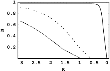
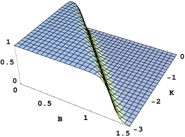
Figure 1: The negativity vs. the nonlinear couplings constant $K$ for different temperature $T$ (from top to bottom, $T$ equals $0.05$, $0.6$, $1.0$), the magnetic field $B=0$.

Figure 2: (Color on line)The negativity vs. the nonlinear couplings constant $K$ and the magnetic field $B$, the temperature $T=0.1$.

We perform the numerical diagonalization of the density matrix and the numerical results of the entanglement measure are presented in figures from Fig.1-Fig.3. Fig.1 shows the plot of the negativity as a function of the nonlinear couplings constant $K$ for different temperature $T$ when $B=0$. From the figure we can see that the thermal entanglement increases with the increasing $|K|$ and demonstrates a different evolvement curve for different temperature. When $B=0$, $K<0$ and the temperature is close to absolute zero, the state $|\Psi_{8}^{+}\rangle$ is seen to be the ground state, which is a entangled state, so the negativity is not equal to zero (in fact the negativity is equal to $0.972$) and it decreases with the decreasing of $|K|$. Only when the nonlinear couplings $|K|$ are larger than a certain critical value does the entanglement exist. For $T=0.6$, the critical value of $|K|$ is smaller than that for $T=1.0$. We can also see that the maximum value that the negativity can arrive at gets smaller with the increasing temperature for a fixed $|K|$ and the system can hold high entanglement in a quite broader area of the nonlinear couplings $K$ when the temperature is close to zero.

The negativity as a function of the nonlinear couplings constant $K$ and the magnetic field $B$ is plotted in Fig.2 when $T=0.1$. The magnetic field plays a negative role for the negativity at a fixed temperature, this can be seen from the figure. There should exist a competition between the magnetic field and the nonlinear couplings $|K|$. The critical magnetic field for various $|K|$ is different and it increases nearly linearly when $|K|$ increases. The negativity will arrive at zero when the magnetic field has a very large value. This is very easily understood since the term $K(S_{1}\cdot S_{2})^{2}$ in the Hamiltonian can be ignored when $B$ is very large, thus the system is unentangled.

Figure 3: The negativity vs. the temperature for different magnetic field $B$ (from top to bottom, $B$ equals $0.2$, $1.0$, $1.5$), nonlinear couplings constant $K=-3$.

In Fig.3, the plot of the negativity as a function of the temperature for different magnetic field is given. When $B$ is close to zero, the state $|\Psi_{8}^{+}\rangle$ is seen to be the ground state in which the negativity is about $0.972$ at $T=0$. As the temperature increases, $N$ rapidly decreases due to the mixing of the excited states with the ground state. For a higher value of the magnetic field $B$ (say $B=1.5$), the state $|\Psi_{2}\rangle$ becomes the ground state and there is no entanglement at $T=0$. However we may increase the entanglement by increasing the temperature $T$ in order to bring the entangled eigenstates such as $|\Psi_{8}^{\pm}\rangle$ into mixing with the ground state. We also found that the critical temperature is almost the same for different external field. The change in negativity as $T$ increases from absolute zero is due to population of excited levels. These results are consistent with those found in our previous paper[6, 13].

4 Conclusions

We investigate qualitatively (not quantitatively) the effects of nonlinear couplings and external magnetic field on the thermal entanglement in a two-spin-qutrit system in terms of the measure of entanglement called “negativity”. We find that the nonlinear couplings favor the thermal entanglement. Only when the nonlinear couplings $|K|$ are larger than a certain critical value does the entanglement exist. Increasing the nonlinear couplings $|K|$ increases the critical magnetic field, but the critical temperature is almost the same for different external magnetic field at a fixed nonlinear couplings constant.

References

- [1] E. Schrödinger, Naturwiss 23 (1935) 807; 23(1935) 823; 23(1935) 844.
- [2] A. Einstein, B. Podolsky, N. Rosen, Phys. Rev. 47 (1935) 777.
- [3] M. C. Arnesen, S. Bose and V. Vedral, Phys. Rev. Lett. 87 (2001) 017901.
- [4] K. M. O Connor and W. K. Wootters, Phys. Rev. A 63 (2001) 052302.
- [5] X. Wang, Phys. Rev. A 66 (2002) 044305 ; X. Wang, Phys. Rev. A 66 (2002) 034302.
- [6] G. F. Zhang, J. Q. Liang, Q. W. Yan, Chin. Phys. Lett. 20 (2003) 452.
- [7] X. Wang, Phys. Rev. A 64(2001) 012313; G. L. Kamta and A. F. Starace, Phys. Rev. Lett. 88 (2002) 107901.
- [8] G. F. Zhang and S. S. Li, Phys. Rev. A 72 (2005) 034302.
- [9] D. Gunlycke, V. M. Kendon, and V. Vedral, Phys. Rev. A 64 (2001) 042302.
- [10] S. Mancini, and S. Bose, Phys. Rev. A 70 (2004) 022307.
- [11] M. A. Nielsen, e-print quant-ph/0011036.
- [12] V. Scarani et al., Phys. Rev. Lett. 88 (2002) 09790.
- [13] G. Zhang, S. Li and J. Liang, Optical Communications 245 (2005) 457-463.
- [14] G. F. Zhang, and S. S. Li, will appear in Eur. Phys. J. D.
- [15] D. Jaksch, C. Bruder, J. I. Cirac, C. W. Gardiner and P. Zoller, Phys. Rev. Lett. 81 (2003) 3108.
- [16] S. K. Yip, Phys. Rev. Lett. 90 (1998) 250402.
- [17] A. Peres, Phys. Rev. Lett. 77 (1996) 1413; M. Horodecki, P. Horodecki, and R. Horodecki, Phys. Lett. A 223 (1996) 1.
- [18] G. Vidal and R. F. Werner, Phys. Rev. A 65 (2002) 032314.
- [19] K. Zyczkowski, P. Horodecki et al., Phys. Rev. A 58 (1998) 883.