On Algebraic and Quantum Random Walks

Abstract

Algebraic random walks (ARW) and quantum mechanical random walks (QRW) are investigated and related. Based on minimal data provided by the underlying bialgebras of functions defined on e. g the real line R, the abelian finite group $\textbf{Z}_{N}$, and the canonical Heisenberg-Weyl algebra hw, and by introducing appropriate functionals on those algebras, examples of ARWs are constructed. These walks involve short and long range transition probabilities as in the case of R walk, bistochastic matrices as for the case of $\textbf{Z}_{N}$ walk, or coherent state vectors as in the case of hw walk. The increase of classical entropy due to majorization order of those ARWs is shown, and further their corresponding evolution equations are obtained. Especially for the case of hw ARW, the diffusion limit of evolution equation leads to a quantum master equation for the density matrix of a boson system interacting with a bath of quantum oscillators prepared in squeezed vacuum state. A number of generalizations to other types of ARWs and some open problems are also stated. Next, QRWs are briefly presented together with some of their distinctive properties, such as their enhanced diffusion rates, and their behavior in respect to the relation of majorization to quantum entropy. Finally, the relation of ARWs to QRWs is investigated in terms of the theorem of unitary extension of completely positive trace preserving (CPTP) evolution maps by means of auxiliary vector spaces. It is applied to extend the CPTP step evolution map of a ARW for a quantum walker system into a unitary step evolution map for an associated QRW of a walker+quantum coin system. Examples and extensions are provided.

1 Introduction

Random walks formulated in an algebraic framework[1, 2, 3, 4] of finite groups, bialgebras and operator algebras as well as in the framework of Quantum Mechanics[5]$-$[13], and references therein), are investigated. Minimal data for such constructions consist of a bialgebra[14] and an integral (functional) defined on it, or alternatively of some Lie algebra, and two quantum systems modelling the walker and the coin system, together with a map modelling the coin tossing, that decides probabilistically the stepping of the walker.

Examples of ARWs treated in the following subsections are walks on algebras of functions on R, on ${\textbf{Z}}_{N}$, and on the canonical algebra Heisenberg-Weyl hw[15](section 2). For those walks we show how to define the entropy functional of their respective integral and/or Markov transition operator, and how to deduce that these are entropy increasing random walks by using arguments based on the interrelations relations between majorization bistochastic matrices and entropy[16, 17, 18, 19]. Moreover, a number theoretic decomposing of ARW on ${\textbf{Z}}_{N}$ is analysed, that is called prime decomposition[20], and refers to its factorization into products of similar smaller ${\textbf{Z}}_{N}$-walks. Mathematically this decomposition is based on the Chinese Remainder Theorem and the co-associativity property. Also for the ARWs on R, in addition to the usual case of short range walk with nearest neighbor (NN) transitions (Polya walk)[21], we discuss in our algebraic framework the cases of: i) the NN centrally biased random walk (Gillis walk)[22] and the case of symmetric random walk with exponentially distributed steps (Linderberg-Shuler:LS walk)[23]. Finally, for the hw ARW, where its functional is constructed by means of the eigenstates of the annihilation operator of that algebra i.e the family of coherent state vectors[24, 25], the continuous time, or diffusion like limit, is obtained[15]. This limit results into a trace preserving quantum master equation[26, 27] for the density matrix of a quantum boson system, which physically is identified with the evolution equation of an open quantum boson system interacting coherently with a classical electric field and incoherently (dissipative interaction) with a bath of quantum oscillators rigged initially into a squeezed vacuum state (squeezed white noise)[28, 29, 30].

Section 3, gives a concise prescription of the concept of QRW, using the example of QRW on integers as paradigm[13]. It briefly explains the notion of quantum coin system and the coin tossing map, and summarizes two emblematic properties of that walk, namely the quadratic enhancement of its diffusion rate due to quantum entanglement between the walker and coin systems, and the entropy increase without majorization effect of its probability distributions (pd). This section ends with a group theoretical scheme of classification of various known QRWs.

In section 4, a relation connecting ARW and QRW is put forward. The connection is grounded on the theorem due to Naimark that asserts the possibility of implementing in a unitary way a CPTP map operating on e.g the density operator of a quantum system[31]. This unitary extension is realized in the original vector space of the density operator augmented by an auxiliary vector space, the ancilla space in the terminology of Quantum Information theory[32]. Applied in the context of CPTP of a ARW, the ancilla space is identified with the quantum coin state space of a QRW. The Kraus generators determining the CPTP map of a ARW serve to built, albeit in non unique way, the unitary evolution operator of the associated QRW. This section concludes with the example of an explicit construction of a QRW associated to the hw ARW, of section 2.

Finally, section 4, summarized some of the results and gives some prospected applications of the ARW-QRW concepts and formalism.

2 Algebraic Random Walks

2.1 The case of R

Proposition 1. Let the bialgebra of real formal power series $H\equiv Fun(\mathbf{R})$ generated by the coordinate function $X,$ and let the positive definite functional $\phi:H\rightarrow\mathbf{R}$, defined as $\phi=\sum_{i\in Z}p_{i}\phi_{\alpha_{i}},$ with $0\leq p_{i}\leq 1,\sum_{i\in Z}p_{i}=1,$ where $\phi_{\alpha_{i}}(f(x))=f(\alpha_{i}),$ the functional that evaluates any function $f\in H,$ at the point $\alpha_{i}=i\alpha,$ defined for some step $\alpha\in$ $\mathbf{R}_{+},$ for $i\in Z.$ The $n$-step convoluted functional becomes

$$\phi^{\ast n}=\sum_{i\in Z}p_{i}^{(n)}\phi_{\alpha_{i}}=\widetilde{\phi}^{T}D^{n-1}p,$$ (1)

where $p^{(n)}=D^{n-1}p^{(1)},$ with the stochastic column vectors $p^{(k)}=(p_{i}^{(k)})_{i\in Z},k=1,2,3,\ldots$ and initially $p^{(1)}\equiv p=(p_{i})_{i\in Z}$. Also $D=(D_{ij})=(p_{i-j}),$ $i,j\in Z$ a bistochastic infinite matrix (delta matrix), and $\widetilde{\phi}=(\phi_{\alpha_{i}})_{i\in Z}$ a column vector. Majorization ordering among pd’s is valid at each step i.e $p^{(n+1)}\prec p^{(n)},$ and consequently the ARW is entropy increasing, namely, $S(\phi^{\ast n+1})\geq S(\phi^{\ast n}),$ $S(T_{\phi}^{n+1})\geq S(T_{\phi}^{n}),$ where $S(\phi^{\ast n})\equiv S(T_{\phi}^{n})\equiv$ $S(p^{(n)}),$ with $S(x)$ any Shur-convex function e.g the classical entropy i.e $S(x)=-\sum_{i}x_{i}\log x_{i}.$

Proof: Operating with convoluted functionals on some function $f\in H,$([33, 34],[35, 36, 37, 38],[39, 40]) yields

$$\phi^{\ast 2} =(\phi\otimes\phi)\circ\Delta=\sum_{i,j\in Z}p_{i}^{(1)}p_{j}^{(1)}\phi_{\alpha_{i}+\alpha_{j}}$$

$$=\sum_{k,j\in Z}p_{i}^{(1)}p_{k-i}^{(1)}\phi_{\alpha_{k}}\equiv\sum_{k,j\in Z}p_{i}^{(1)}D_{ki}\phi_{\alpha_{k}}=\widetilde{\phi}^{T}Dp.$$ (2)

By induction we obtain the aimed relation $\phi^{\ast n}=\widetilde{\phi}^{T}p^{(n)}=\widetilde{\phi}^{T}D^{n-1}p^{(1)}.$ Two important properties of the delta matrix are: i) bistochasticity, i.e the column and row sums is one, which is expressed by means of the column vector of units $e=(\ldots,1,1,1,\ldots),$ that is left and right eigenvector of $D,$ i.e $De=e,$ $e^{T}=e^{T}D,$ and ii) the shift property i.e $D_{i,j}=p_{i-j}=p_{i+1-(j+1)}=D_{i+1,j+1}.$ This property in the case of ARW in $Z$ governed by a pd with finite support, or in the case of a $N\subset Z$ finite dimensional walk (see remark below), amounts to a bistochastic matrix $D.$

The functional of the walk at each time step $\phi^{\ast n}=\sum_{i\in Z}p_{i}^{(n)}\phi_{\alpha_{i}},$ is characterized by the pd $p^{(n)}=(p_{i}^{(n)})_{i\in Z}$ , which in turn is determined by the bistochastic matrix $D$ i.e $\ p^{(n)}=Dp^{(n-1)}=D^{n-1}p^{(1)}.$ Let us assume that the pd’s are of finite support (but see remark below), then by invocation of the theorem stating that two discrete pd’s $x=(x_{m})_{m},$ $y=(y_{k})_{k},$ that are connected by a bistochastic matrix $D$ i.e $x=Dy,$ are ordered by majorization [16, 17, 18, 19] i.e $x$ $\prec y$, we conclude that the sequence of pd’s $\{p^{(1)},p^{(2)},p^{(3)},\ldots\}$ , of site occupation probabilities resulting at each time step during the evolution of the walk is partially ordered by majorization i. e $p^{(n)}\prec p^{(n-1)},$ $n=1,2,3,\ldots$ .

Let us adopt now the definition of the entropy of a functional to be the entropy of the pd that determines that functional i.e we set $S(\phi^{\ast n})\equiv S(T_{\phi}^{n})\equiv$ $S(p^{(n)}),$ or more generally we do so for any convex function $S:\mathbf{R}\rightarrow\mathbf{R}$ of the type of the so called Shur-convex functions e.g the classical Shannon entropy $S(p)=\sum_{i}p_{i}\log p_{i}$, or the functions $F(p)=\sum_{i}p_{i}^{k}$, for any constant $k\leq 1$, or $F(p)=-\prod_{i}p_{i}$[17].

By virtue of the theorem stating that $x$ $\prec y$ implies $F(x)<F(y)$ , where $F(x)=\sum_{i}f(x_{i}),$ for any convex function $f:\mathbf{R}\rightarrow\mathbf{R,}$ or otherwise said that the convex functions isotonic to majorization[17], we conclude that for the pd resulting from the random walk the majorization ordering is valid at each step i.e. $p^{(n)}\prec p^{(n-1)},$ $n=1,2,3,\ldots$ , and this implies ordering for e.g their entropies i.e. $S(p^{n})>S(p^{n-1}),$ and similarly for their functionals and transition operators. As majorization order implies entropy increase, it is considered as a measure of disorder, and this allow us to conclude the ARW are getting more disordered in the course of time with respect to their site-visiting pd’s, which are getting more entropic, approaching, if left uninterrupted, to the uniform distribution of maximal entropy.                                                                                                             $\square$

Remarks: 1) The assumption in the previous proof about the support of the pd’s been finite is not actually necessary. In fact in the proof given by Hardy et. al [41]  is stated that given $p\prec q$ for finite sequence of $q,p$ pd’s, use of Muirhead’s algorithm leads to a bistochastic matrix $A,$ such that $q=Ap,$ and then the proposition: $H(Ap)\geq H(p)$ for $\ H$ information/entropy or more generally a Shur convex function, is applied. This proof is constructive and builds $A$ in a number of steps not greater than the lengths of $p,$ $q$, therefore for infinite pd’s a theorem not using bistochastic operators for the characterization of majorization is needed. Such a theorem is provided in [42] .

2) For the above proposition the corresponding Markov transition operator defined as $T_{\phi}=(\phi$ $\otimes id)\circ\Delta,$ is equal to $T_{\phi}=\sum_{i\in Z}p_{i}e^{\alpha_{i}\frac{d}{dx}}.$ For the simplest case of $p_{\pm}=(p,1-p),$ $\alpha_{\pm}=\pm\alpha,$ and all other $p$’s and $\alpha^{\prime}$ s been zero, the continues limit $lim_{n\rightarrow\infty}=(T_{\phi})^{n}\equiv T_{\phi}^{\infty}$  has been obtained that leads to a diffusion equation[33, 3, 4, 15] .

3) The above general algebraic setting implies that the stepping probability matrix $D=(D_{ij})=(p_{i-j}),$ $i,j\in\mathbf{Z,}$ would be expanded in the enveloping algebra $\mathcal{U}(\mathbf{e}(2))$ of the Euclidean Lie algebra $\mathbf{e}(2)\thickapprox\mathbf{iso}(2)$, spanned by monomials of its generators $\{E_{+},E_{-},L\},$ that satisfy the defining commutation relations [43]

$$[E_{+},E_{-}]=0,\qquad[L,E_{\pm}]=\pm E_{\pm}.$$ (3)

An irreducible matrix representation of those generators in the Hilbert space $\mathcal{H}\equiv l_{2}(\mathbf{Z})$ spanned by the eigenvectors of the ”distance operator” $L,$ is useful in expressing the $D$ matrix for various random walks, and look for solutions by means of e.g the Fourier method. This irrep in the canonical basis of $\mathcal{H},$ and using the same symbol for abstract generators and their matrices reads:

$$L=\sum_{m\in Z}me_{m}e_{m}^{\dagger},\text{ \ \ }E_{\pm}=\sum_{m\in Z}e_{m\pm 1}e_{m}^{\dagger}.$$ (4)

Next we present three different random walks in $\mathbf{R,}$ that can be used as show cases of the scheme of ARW presented here. In these concrete examples the defining the walk transition probability matrix $D,$ is written as an element of the $\mathcal{U}(\mathbf{e}(2))$ algebra. No attempt will be made to give an algebraic solution for the problem of finding the $n$ th$-$step site occupancy probability distribution, as this can be solved by other means.

The examples include: i) the simplest case of symmetric nearest-neighbor (NN) random walk (Polya-walk[21]); one of its deformations, ii) the NN centrally (site $n=0)$ biased random walk (Gillis-walk[22]), which refers to a solvable case of a walk with no translational invariance, and stepping probabilities with a bias which has  power law decay, or more specifically which decays in proportion from the origin of coordinates. The $\ \varepsilon-$deformation parameter is chosen so that when $\varepsilon>0,$ the walk is biased to enhance returns to the origin, while if $\varepsilon<0,$ escape from the origin is enhanced, and iii) a symmetric random walk with non- nearest-neighbor transitions with transition step length decaying according to an exponential law (LS-walk[23]). Explicitly we have:

1)

Polya-walk: symmetric nearest-neighbor(NN) random walk with Markov transition operator

$$D_{P}=\frac{1}{2}(E_{-}+E_{+})$$ (5)

with matrix elements the inter-site transition probabilities

$$D_{P}(l,l^{{}^{\prime}})=\frac{1}{2}\delta_{l,l^{{}^{\prime}}-1}+\frac{1}{2}\delta_{l,l^{{}^{\prime}}+1}.$$ (6)

2) Gillis-walk: nearest-neighbor centrally (site $n=0)$ biased random walk with Markov transition operator

$$D_{G}=D_{G}(\varepsilon)=\frac{1}{2}(E_{-}+E_{+})+(E_{-}-E_{+})\frac{\varepsilon}{2N}P_{0}^{\bot},\text{ \ \ \ \ \ \ \ \ \ }-1<\varepsilon<1$$ (7)

where $P_{0}=e_{0}e_{0}^{\dagger},$ $P_{0}^{\bot}=1-P_{0},$ the projection operators in the vector $e_{0},$ and its orthogonal subspace respectively in $l_{2}(\mathbf{Z}),$ and with matrix elements the inter-site transition probabilities

$$D_{G}(l,l^{{}^{\prime}}) =\frac{1}{2}(1+\frac{\varepsilon}{l^{{}^{\prime}}})\delta_{l,l^{{}^{\prime}}-1}+\frac{1}{2}(1-\frac{\varepsilon}{l^{{}^{\prime}}})\delta_{l,l^{{}^{\prime}}+1},\text{ \ \ \ \ \ \ \ }l^{{}^{\prime}}\neq 0$$ (8)

$$D_{G}(l,0) =\frac{1}{2}\delta_{l,-1}+\frac{1}{2}\delta_{l,1}.$$ (9)

3) LS-walk: symmetric random walk with exponentially distributed steps with Markov transition operator

$$D_{LS}=D_{LS}(\varepsilon)=\frac{e^{\varepsilon}-1}{2}\sum_{k\in Z_{>0}}e^{-k\varepsilon}(E_{-}^{k}+E_{+}^{k})$$ (10)

with matrix elements the inter-site transition probabilities

$$D_{LS}(l,l^{{}^{\prime}}) =\frac{e^{\varepsilon}-1}{2}e^{-\left|l-l^{{}^{\prime}}\right|\varepsilon},\qquad\left|l-l^{{}^{\prime}}\right|>0$$ (11)

$$=0,\qquad\qquad\qquad\qquad\ l=l^{{}^{\prime}}.$$

Use of the eigenvector equations $E_{\pm}e=e,$ $\ e^{\dagger}=e^{\dagger}E_{\pm},$ leads to the conclusion that the transition matrices of the Polya, and LS random walks i.e the matrices $D_{P},D_{R},$ and $D_{LS}$ respectively are bistochastic, while that of the Gillis walk $D_{G},$ is column stochastic. Also from the definitions the following two limits are deduced: $\lim_{\varepsilon\rightarrow 0}D_{G}(\varepsilon)=\lim_{\varepsilon\rightarrow\infty}D_{LS}(\varepsilon)=D_{P}.$

Generalizations: The 2D generalized Gillis random walk with entanglement. This model describes a 2D NN random walk with a biased towards a point placed at $(m_{1},m_{2})$ coordinates on the plane. The bias is an attractive or repelling one depending on the sign of two parameters $(\varepsilon_{1},\varepsilon_{2})$  in reference to the motion along $x,y$   axes respectively, and its strength decays following an inverse power law with characteristic exponents ($a_{1},a_{2})$ correspondingly. This is summarized by writing explicitly all parameters in the Markov transition operator $D_{G}^{2D}(\varepsilon_{1},$  $m_{1},$ $a_{1};\varepsilon_{2},\ m_{2},a_{2}),$ and their domain of values $\{\varepsilon_{j},$  $m_{j},$ $a_{j}\}\in\{$ $(-1,1),\mathbf{Z},\mathbf{Z}_{+}\},$ $j=1,2.$ The transition matrix along each axis is

$$D_{G}(\varepsilon_{j},m_{j},a_{j})=\frac{1}{2}(E_{-}+E_{+})+(E_{-}-E_{+})\frac{\varepsilon_{j}}{2(N-m_{j}\mathbf{1})^{a_{j}}}P_{j}^{\bot},\text{ \ \ \ \ }j=1,2$$ (12)

where $P_{j}=e_{j}e_{j}^{\dagger},$ $P_{j}^{\bot}=1-P_{j},$ the projection operators in the vector $e_{j},$ and its orthogonal subspace respectively in $l_{2}(\mathbf{Z}).$ The 2D transition operator consists of an entangled[32] convex combination of two factorizable 1D transition operators  with the parameters of position of bias site, characteristic decay exponent, and decay strength c.f $\ \{m_{j},a_{j},\varepsilon_{j},\},$ $j=1,2$  interchanged, it reads ($0\leq q\leq 1)$

$$D_{G}^{2D} =qD_{G}(\varepsilon_{1},m_{1},a_{1})\otimes D_{G}(\varepsilon_{2},m_{2},a_{2})$$

$$+(1-q)D_{G}(\varepsilon_{2},m_{2},a_{2})\otimes D_{G}(\varepsilon_{1},m_{1},a_{1}),$$ (13)

with matrix elements the inter-site transition probabilities

$$D_{G}^{2D}(l_{1},l_{1}^{{}^{\prime}};l_{2},l_{2}^{{}^{\prime}}) =q\frac{1}{4}\left[1+\frac{\varepsilon_{1}}{(l_{1}^{{}^{\prime}}-m_{1})^{a_{1}}}\right]\left[1+\frac{\varepsilon_{2}}{(l_{2}^{{}^{\prime}}-m_{2})^{a_{2}}}\right]\delta_{l_{1},l_{1}^{{}^{\prime}}-1}\delta_{l_{2},l_{2}^{{}^{\prime}}-1}$$

$$+(1-q)\frac{1}{4}\left[1+\frac{\varepsilon_{2}}{(l_{1}^{{}^{\prime}}-m_{2})^{a_{2}}}\right]\left[1+\frac{\varepsilon_{1}}{(l_{2}^{{}^{\prime}}-m_{1})^{a_{1}}}\right]\delta_{l_{1},l_{1}^{{}^{\prime}}-1}\delta_{l_{2},l_{2}^{{}^{\prime}}-1,}$$ (14)

with $(l_{1}^{{}^{\prime}},l_{2}^{{}^{\prime}})\neq(m_{1},m_{2}),$ for the $q$  component and $(l_{1}^{{}^{\prime}},l_{2}^{{}^{\prime}})\neq(m_{2},m_{1}),$ for the $(1-q)$ component of the convex combination. Also

$$D_{G}^{2D}(l_{1},l_{2}^{{}^{\prime}} =m_{1,2};l_{1},l_{2}^{{}^{\prime}}=m_{2,1})=q(\frac{1}{2}\delta_{l_{1},m_{1}-1}+\frac{1}{2}\delta_{l_{1},m_{1}+1})$$

$$.(\frac{1}{2}\delta_{l_{2},m_{2}-1}+\frac{1}{2}\delta_{l_{2},m_{2}+1}) +(1-q)(\frac{1}{2}\delta_{l_{1},m_{2}-1}+\frac{1}{2}\delta_{l_{1},m_{2}+1})$$

$$.(\frac{1}{2}\delta_{l_{2},m_{1}-1}+\frac{1}{2}\delta_{l_{2},m_{1}+1}).$$ (15)

the matrix elements with $(l_{1}^{{}^{\prime}},l_{2}^{{}^{\prime}})=(m_{1},m_{2}),$ for the $q$  component and $(l_{1}^{{}^{\prime}},l_{2}^{{}^{\prime}})=(m_{2},m_{1}),$ for the $(1-q)$ component of the convex combination. The role of bias and that of the entanglement of the two 1D walks, can be investigated in an algebraic manner in terms of tensor product representations of the $\mathbf{iso(2)}$ algebra, and it will be given elsewhere[44].

2.2 The case of ${\bf Z_{N}}$

In this section we give a brief study of algebraic random walks on abelian groups $\mathbf{Z}_{N}$ [3], using their underlying bialgebra structure, and further investigate possible forms of their decomposition into simpler and dimensionally lower ARWs, based on number theoretic properties of $N$.

Proposition 2. Let the multiplicative abelian group $\mathbf{Z}_{N}=\{e,g,g^{2},\ldots,g^{N-1}\}$ and the bialgebra $H\equiv\mathbf{C(\mathbf{Z}_{N})}\equiv Fun(\mathbf{Z}_{N})=\mathbf{C}-span\langle\left\{g^{i}\right\}_{i=0}^{N-1}\rangle$, with dual algebra $H^{\ast}\equiv\mathbf{CZ}_{N}\equiv Fun(Z_{N}^{\ast})$,  with pairing given by evaluation. Let the positive definite functional (state) of a $\mathbf{Z}_{N}$ random walk $\phi=\sum_{i\in[0,N-1]}p_{i}g^{i},$ identified as weighted sum of elements of $H,$ with $0\leq p_{i}\leq 1,\sum_{i\in[0,N-1]}p_{i}=1.$ By means of the column vectors $P=(p_{i})_{i\in[0,N-1]},G=(g^{i})_{i\in[0,N-1]},$we write it as $\phi=G^{T}P,$ where $T$ denotes transpose. Then the $n$-th step convolution becomes $\phi^{\ast n}=G^{T}D^{n-1}P$, where    $D=(D_{ij})=(p_{i-j\mid\operatorname{mod}N}),$ $i,j\in[0,N-1]$ a circulant bistochastic matrix, to be called delta matrix.

Proof: Straightforward (c.f. [3]).

Remarks: 0) The delta matrix is more precisely a circulant bistochastic matrix[45], that can be treated as an element of finite Heisenberg group$H_{N}$ [20], and this leads to an explicit solution for the dynamics of $\mathbf{Z}_{N}$ walk.

1) Recall the following version of the Chinese Remainder Theorem (CRT)[46]: let $N=N_{1}N_{2}$, the decomposition of positive integer $N,$ into product of coprimes $N_{1},N_{2},$ then working with the abelian additive groups of numbers $Z_{N_{1,2}},$ $\operatorname{mod}N_{1,2}$ respectively, we can introduce the unique bijection

$$\delta:Z_{N}\longrightarrow Z_{N_{1}}\times Z_{N_{2}},\text{ \ \ }\delta(x)=(x-\rho N_{1},x-\sigma N_{2}),$$ (16)

$\rho,\sigma\in Z,$ that maps the numbers of $Z_{N},$ into the ordered pair of its remainders after division by $N_{1},N_{2}.$ Its dual map is the inverse $\mu\equiv\delta^{-1}=Z_{N_{1}}\times Z_{N_{2}}\longrightarrow Z_{N},$which constructs the unique number $x$ from its remainders $(a,b)$, with respect to the divisors $N_{1},N_{2},$ as $\mu(a,b)=aN_{1}^{\varphi(N_{1})}+bN_{2}^{\varphi(N_{2})}=x,$ where $\varphi(c)=\#\left|c\geq m\in Z_{+};GCD(m,c)=1\right|,$ the Euler function of given integer $c,$ that equals the number of co-primes less or equal to $c.$

2) The same factorization is valid for abelian multiplicative groups i.e $\mathbf{Z}_{N}\cong\mathbf{Z}_{N_{1}}\bigotimes\mathbf{Z}_{N_{2}},$ if $N=N_{1}N_{2},$ and $N_{1},N_{2},$ are relative primes.

3) Let for later use introduce now the map $\delta\longrightarrow V_{\delta},$ that uniquely determines from the CRT bijection $\delta,$ with $\delta(i)=(i_{1},i_{2}),$ the isometric matrix $V_{\delta}:\mathbf{C}_{N}\longrightarrow\mathbf{C}_{N_{1}}\otimes\mathbf{C}_{N_{2}},$ written in the canonical basis as[20]

$$V_{\delta}=\sum_{i\in Z_{N}}e_{\delta(i)}e_{i}^{\dagger}\equiv\sum_{i\in Z_{N}}(e_{i_{1}}\otimes e_{i_{1}})e_{i}^{\dagger},$$ (17)

and its inverse

$$V_{\delta}^{\dagger}=V_{\delta^{-1}}=\sum_{i_{1}\in Z_{N_{1}},i_{2}\in Z_{N_{2}}}e_{\delta^{-1}(i_{1},i_{2})}e_{(i_{1},i_{2})}^{\dagger}\equiv\sum_{i_{1}\in Z_{N_{1}},i_{2}\in Z_{N_{2}}}e_{\delta^{-1}(i_{1},i_{2})}(e_{i_{1}}^{\dagger}\otimes e_{i_{1}}^{\dagger}),$$ (18)

for which we have $V_{\delta}V_{\delta}^{\dagger}=V_{\delta}V_{\delta^{-1}}=V_{\delta\circ\delta^{-1}}=V_{id\times id}=\mathbf{1}_{\mathbf{C}_{N_{1}}}\otimes\mathbf{1}_{\mathbf{C}_{N_{2}}},$ and $V_{\delta}^{\dagger}V_{\delta}=V_{\delta^{-1}}V_{\delta}=V_{\delta^{-1}\circ\delta}=V_{id}=\mathbf{1}_{\mathbf{C}_{N}}.$

Notation: in the sequel and in order to distinguish the space dimensionality $N,$ referring to certain e.g functional, operator, probability vector, co-multiplication etc, we will denote it by $\phi_{[N]},T_{[N]},$ and $P_{[N]}$ respectively. We can now state two necessary and sufficient conditions, in order to obtain an isomorphic prime decomposition of a $\mathbf{Z}_{N}$ ARW governed by a pd $P_{[N]},$ into a product of two others ARWs $\mathbf{Z}_{N_{1}},$ $\mathbf{Z}_{N_{2}},$ with respective pd’s $P_{[N]}=P_{[N_{1}]}\otimes P_{[N_{2}]}$. The first condition is number theoretic and is about the compositeness of the dimension number $N$ of the probability distribution $P_{[N]}$ that generates the ARW on $\mathbf{Z}_{N}$, while the second condition is about its factorization into a tensor product of two pd’s of appropriate dimensions.

Proposition 3. i) Let $N=N_{1}N_{2}$ be the prime factorization of a positive integer $N,$   then if in addition to the isomorphism of abelian groups of $Z_{N}\approx Z_{N_{1}}\otimes Z_{N_{2}},$ we consider a probability distribution (pd) $P_{[N]}$ factorizable into a product of two others pd’s $P_{[N_{1}]},P_{[N_{2}]},$ namely such that $V_{\delta}P_{[N]}=P_{[N_{1}]}\otimes P_{[N_{2}]},$ or $p_{i}^{[N]}=p_{i_{1}}^{[N_{1}]}p_{i_{2}}^{[N_{2}]},$ then the functional of a $\mathbf{Z}_{N}$ algebraic random walk $\phi_{[N]}=\sum_{i\in Z_{N}}p_{i}^{[N]}g_{[N]}^{i},$ with $0\leq p_{i}^{[N]}\leq 1,\sum_{i\in Z_{N}}p_{i}^{[N]}=1,$ factorizes for every step $n,$ namely $\phi_{[N]}^{\ast n}\approx\phi_{[N_{1}]}^{\ast n}\otimes\phi_{[N_{2}]}^{\ast n},$ and similar factorization is valid for the transition operator i.e $T_{[N]}^{n}\approx T_{[N_{1}]}^{n}\otimes T_{[N_{2}]}^{n}.$

ii) Let $N_{1},$ $N_{2}$ and $N_{3,}$ be the co-prime factors of some positive integer $N$, then the decomposition $Z_{N}\approx Z_{N_{1}}\otimes Z_{N_{2}}\otimes Z_{N_{3}}\approx Z_{N_{1}N_{2}}\otimes Z_{N_{3}}\approx Z_{N_{1}}\otimes Z_{N_{2}N_{3}},$ is co-assosiative[14] as indicated in the last two equations, and if a pd $P_{[N]}$ is considered for which the finest decomposition $V_{\delta}P_{[N]}=P_{[N_{1}]}\otimes P_{[N_{2}]}\otimes P_{[N_{3}]},$ in terms of three others pd’s is true, then the associated $\mathbf{Z}_{N}$ ARW is also decomposed at any step $n,$ namely for its functional and transition operator respectively, the following co-associative factorizations are valid

$$\phi_{[N]}\approx\phi_{[N_{1}]}\otimes\phi_{[N_{2}]}\otimes\phi_{[N_{3}]}\approx\phi_{[N_{1}N_{2}]}\otimes\phi_{[N_{3}]}\approx\phi_{[N_{1}]}\otimes\phi_{[N_{2}N_{3}]},$$ (19)

Proof: i) The $N=N_{1}N$

₂ case: By means of the factorization property of  the pd viz.

$$V_{\delta}P_{[N]} =\sum_{i\in Z_{N}}p_{i}^{[N]}V_{\delta}e_{i}\approx\sum_{i\in Z_{N}}p_{\delta(i)}^{[N]}e_{\delta(i)}=\sum_{i_{1}\in Z_{N_{1}},i_{2}\in Z_{N_{2}}}p_{(i_{1},i_{2})}^{[N]}e_{i_{1}}\otimes e_{i_{2}}$$

$$=\sum_{i_{1}\in Z_{N_{1}},i_{2}\in Z_{N_{2}}}p_{i_{1}}^{[N_{1}]}p_{i_{2}}^{[N_{2}]}e_{i_{1}}\otimes e_{i_{2}}=P_{[N_{1}]}\otimes P_{[N_{2}]},$$ (20)

we deduce that

$$V_{\delta}D_{[N]}V_{\delta}^{\dagger} =\sum_{i,j\in Z_{N}}p_{(i-j)}^{[N]}V_{\delta}e_{i}e_{j}^{\dagger}V_{\delta}^{\dagger}$$

$$\approx\sum_{i_{1}\in Z_{N_{1}},i_{2}\in Z_{N_{2}}}p_{\delta(i-j)}^{[N]}e_{i_{1}}\otimes e_{i_{2}}.e_{i_{1}}^{\dagger}\otimes e_{i_{2}}^{\dagger}=D_{[N_{1}]}\otimes D_{[N_{2}]},$$ (21)

and therefore $V_{\delta}D_{[N]}^{n}V_{\delta}^{\dagger}\approx D_{[N_{1}]}^{n}\otimes D_{[N_{2}]}^{n},$ for the delta matrix. This yields the factorization of the functional

$$\phi_{[N]} = G_{[N]}^{T}P_{[N]}=G_{[N]}^{T}V_{\delta}^{\dagger}V_{\delta}P_{[N]}$$ (22)

$$\approx (V_{\delta}G_{[N]}^{T})^{\dagger}(V_{\delta}P_{[N]})=G_{[N_{1}]}^{T}{}^{\dagger}\otimes G_{[N_{2}]}^{T}{}^{\dagger}.P_{[N_{1}]}\otimes P_{[N_{2}]}=\phi_{[N_{1}]}\otimes\phi_{[N_{2}]},$$

and similarly for the transition operator (with $\tau(x\otimes y)=y\otimes x$ )

$$T_{[N]} = (id\otimes\tau\otimes id)\circ(\phi_{[N]}\otimes id_{[N]})\circ\Delta_{[N]}$$ (23)

$$\approx (\phi_{[N_{1}]}\otimes id_{[N_{1}]}\otimes\phi_{[N_{2}]}\otimes id_{[N_{1}]})\circ(\Delta_{[N_{1}]}\otimes\Delta_{[N_{1}]})\approx T_{[N_{1}]}\otimes T_{[N_{2}]}.\qquad$$

ii) The $N=N_{1}N_{2}N_{3}$ case: Applying the CRT to $N,$ in two different ways yields for the abelian group $Z_{N}$ two factorizations i.e $Z_{N}\approx Z_{N_{1}}\otimes Z_{N_{2}}\otimes Z_{N_{3}}\approx Z_{N_{1}N_{2}}\otimes Z_{N_{3}}\approx Z_{N_{1}}\otimes Z_{N_{2}N_{3}}.$ This can equivalently be expressed by means of the bijection $\delta,$ as

$$(\delta_{[N_{1},N_{2}]}\otimes id)\circ\delta_{[N_{1}N_{2},N_{3}]}=(id\otimes\delta_{[N_{2},N_{3}]})\circ\delta_{[N_{1},N_{2}N_{3}]}.$$ (24)

Performing the factorization of the pd $P_{[N]},$ as before twice we have

$$(V_{\delta_{[N_{1},N_{2}]}}\otimes\mathbf{1})V_{\delta_{[N_{1}N_{2},N_{3}]}}P_{[N]}=P_{[N_{1}]}\otimes P_{[N_{2}]}\otimes P_{[N_{3}]}$$ (25)

which implies that

$$(V_{\delta_{[N_{1},N_{2}]}}\otimes\mathbf{1})V_{\delta_{[N_{1}N_{2},N_{3}]}}D_{[N]}^{n}((V_{\delta_{[N_{1},N_{2}]}}\otimes\mathbf{1})V_{\delta_{[N_{1}N_{2},N_{3}]}})^{\dagger}\approx D_{[N_{1}]}^{n}\otimes D_{[N_{2}]}^{n}\otimes D_{[N_{3}]}^{n}.$$ (26)

This factorization of the delta matrix leads to an equivalent factorizations of the functional at each time step of the $\mathbf{Z}_{N}$ walk, i.e

$$\phi_{[N]}^{\ast n}\approx\phi_{[N_{1}N_{2}]}^{\ast n}\otimes\phi_{[N_{3}]}^{\ast n}\approx\phi_{[N_{1}]}^{\ast n}\otimes\phi_{[N_{2}N_{3}]}^{\ast n}\approx\phi_{[N_{1}]}^{\ast n}\otimes\phi_{[N_{2}]}^{\ast n}\otimes\phi_{[N_{3}]}^{\ast n}$$ (27)

Similar decompositions can be obtained for Markov transition operators.                                                           $\square$

Remark: Interpretation of this result implies that the original random walk $\mathbf{Z}_{N},$ is isomorphically decomposed into the product of : i) three similar walks $\mathbf{Z}_{N}\cong\mathbf{Z}_{N_{1}}\otimes\mathbf{Z}_{N_{2}}\otimes\mathbf{Z}_{N_{3}},$ ii) or into the product of two walks of dimensions $N_{1}N_{2}$ and $N_{3}$ i.e $\mathbf{Z}_{N_{1}N_{2}}\otimes\mathbf{Z}_{N_{3}}$ and iii) or into the product of two walks of dimensions $N_{1}$ and $N_{2}N_{3}$ i.e $\mathbf{Z}_{N_{1}}\otimes\mathbf{Z}_{N_{2}N_{3}}.$ As an example we take the  $\mathbf{Z}_{6}$ random walk on the vertices of  a canonical hexagon the statistics of which is determined by a $6$-dimension pd vector $P_{[6]}.$ If this pd has been chosen so that there are two other pd’s one 3-dimensional $P_{[3]}$ that generates a $\mathbf{Z}_{3}$ ARW on the vertices of a canonical triangle, and one 2-dimensional  $P_{[2]}$ that generates a $\mathbf{Z}_{2}$ walk on two points, such that  $P_{[6]}=P_{[3]}\bigotimes P_{[2]},$ then we can decompose  the ARW on the canonical hexagon as a product of two walks one  on the triangle times one on the two-point set. Similar interpretations can be given to the prime decomposition of an ARW on  a canonical polygon. E. g  the decomposition $\mathbf{Z}_{60}\cong$ $\mathbf{Z}_{3}\bigotimes\mathbf{Z}_{4}\bigotimes\mathbf{Z}_{5}\cong$ $\mathbf{Z}_{12}\bigotimes\mathbf{Z}_{5}\cong$ $\mathbf{Z}_{3}\bigotimes\mathbf{Z}_{20}$[20].

Problem: Let $N=N_{1}N_{2}$ be the prime factorization of a positive integer $N,$ for which the isomorphism $Z_{N}\approx Z_{N_{1}}\otimes Z_{N_{2}},$ is valid, let us consider an $\mathbf{Z}_{N}$ ARW generated as previously by a pd $P_{[N]}.$ It this pd is not factorizable into a product of two others pd’s as in the remark above, but instead there are two pairs of pd’s $P_{[N_{1}]},$ $P_{[N_{1}]}^{/},$ and $P_{[N_{2}]},$ $P_{[N_{2}]}^{/},$ such that the original pd is a convex combination of them i. e $(0\leq q\leq 1),$

$$V_{\delta}P_{[N]}=qP_{[N_{1}]}\otimes P_{[N_{2}]}+(1-q)P_{[N_{1}]}^{/}\otimes P_{[N_{2}]}^{/}.$$ (28)

In the terminology of quantum information[32], we have here two ARWs $\mathbf{Z}_{N_{1}},\mathbf{Z}_{N_{2}},$ that are classically correlated (cc) and form a probabilistic decomposition of the ARW in $\mathbf{Z}_{N},$ and write symbolically $\mathbf{Z}_{N}\cong q\mathbf{Z}_{N_{1}}\bigotimes\mathbf{Z}_{N_{2}}+(1-q)\mathbf{Z}_{N_{1}}^{/}\bigotimes\mathbf{Z}_{N_{2}}^{/}.$ A number of interesting problems arise in this context: the total dynamics and reduced dynamics of the components of the $\mathbf{Z}_{N}$ walk; the problem of construction of measures of correlations among the components of $\mathbf{Z}_{N}$ walk; the problem of information(majorization) dynamics and information exchange among the pd’s components of the $\mathbf{Z}_{N}$ walk; the problem of asymptotics of the $\mathbf{Z}_{N}$ walk.

2.3 The case of hw-Algebra

A bialgebra [14] ${\mathcal{A}}={\mathcal{A}}(\mu,\eta,\Delta,\epsilon)$ over a field $k$ is a vector space equipped with an algebra structure with homomorphic associative product map $\mu:{\mathcal{A}\/}\times{\mathcal{A}\/}\rightarrow{\mathcal{A}\/}$, and a homomorphic unit map $\eta:k\rightarrow{\mathcal{A}\/}$, that are related by $\mu\circ(\eta\otimes id)=id=\mu\circ(id\otimes\eta)$, together with a coalgebra structure with a homomorphic coassociative coproduct map $\Delta:{\mathcal{A}\/}\rightarrow{\mathcal{A}\/}\otimes{\mathcal{A}\/}$ and a homomorphic counit map $\epsilon:{\mathcal{A}\/}\rightarrow k$, that are related between them by $(\epsilon\otimes id)\circ\Delta=id=(id\otimes\epsilon)\circ\Delta$. Both products satisfy the compatibility condition of bialgebra i.e $(\mu\otimes\mu)\circ(id\otimes\tau\otimes id)\circ(\Delta\otimes\Delta)=\Delta\circ\mu$, where $\tau(x\otimes y)=y\otimes x$ stands for the twist map. If $\eta$ or $\epsilon$ is not defined in ${\mathcal{A}\/}$ we speak about non unital or non counital Hopf algebra.

Suppose we have a functional $\phi:{\mathcal{A}\/}\rightarrow\bf C$, defined on ${\mathcal{A}\/}$, let us define the operator $T_{\phi}:{\mathcal{A}\/}\rightarrow{\mathcal{A}\/}$ as $T_{\phi}=(\phi\otimes id)\circ\Delta$, then $\epsilon\circ T_{\phi}=\phi$, namely the counit aids to pass from the operator to its associated functional. From this relation we can define the convolution product $\psi*\phi$, between functionals as follows [33]:

$$\epsilon\circ T_{\psi}T_{\phi} = \epsilon\circ(\psi\otimes id)\circ\Delta\circ(\phi\otimes id)\circ\Delta$$ (29)

$$= (\phi\otimes\psi)\circ(id\otimes id\otimes\epsilon)\circ(id\otimes\Delta)\circ\Delta$$

$$= (\phi\otimes\psi)\circ\Delta=\phi*\psi\;,$$

and in general $\epsilon\circ T_{\phi}^{n}=\epsilon\circ T_{\phi^{*n}}=\phi^{*n}$. These last relations imply that the transition operators form a discrete semigroup with respect to their composition with identity element $T_{\epsilon}\equiv id$ (due to the axioms of bialgebra) and generator $T_{\phi}$, while the functionals form a dual semigroup with respect to the convolution with identity element $e$ and generator $\phi$, and that these two semigroups are homomorphic to each other.

We recall now the Heisenberg-Weyl algebra $\bf hw$ and its structural maps: this is the algebra of the quantum mechanical oscillator and is generated by the creation, annihilation and the unit operator $\{a^{\dagger},a,{\bf 1\/}\}$ respectively which satisfy the commutation relation (Lie bracket) $[a,a^{\dagger}]={\bf 1\/}$, while ${\bf 1\/}$ commutes with the other elements. This algebra possesses a non counital bialgebra structure [3], chapt. 3), with comultiplication defined as

$$\Delta^{(n-1)}a = n^{-\frac{1}{2}}(a\otimes\cdots\otimes{\bf 1\/}+{\bf 1\/}\otimes a\otimes\cdots\otimes{\bf 1\/}+{\bf 1\/}\otimes\cdots\otimes a)\;,$$

$$\Delta^{(n-1)}a^{\dagger} = n^{-\frac{1}{2}}(a^{\dagger}\otimes\cdots\otimes{\bf 1\/}+{\bf 1\/}\otimes a\otimes\cdots\otimes{\bf 1\/}+{\bf 1\/}\otimes\cdots\otimes a^{\dagger})\;,$$

$$\Delta{\bf 1\/} = {\bf 1\/}\otimes{\bf 1\/}\;,$$ (30)

where as indicated above the $\Delta^{(n-1)}$ maps the creation/annihilation operators into the $n$th fold tensor product of the algebra and adds appropriate factors (also c.f. [47]). Let us also define the number operator $N=a^{\dagger}a$ with the following commutation relations with the generators of $\bf hw$: $[N,a^{\dagger}]=a^{\dagger}\;,[N,a]=-a$. The module which carries the unique irreducible and infinite dimensional representation of the oscillator algebra is the Hilbert-Fock space ${\mathcal{H}}_{F}$ which is generated by a lowest (or ”vacuum” ) state vector $\left|0\right>\in\mathcal{H}_{F}$ and is given as ${\mathcal{H}}_{F}=\{\left|n\right>=\frac{(a^{\dagger})^{n}}{n!}\left|0\right>,n\in{\bf Z}_{+}\}$.

The functionals we intend to use will be defined by means of the canonical coherent state vectors of the $\bf hw$ algebra so in the sequel we give a brief introduction to the concept of coherent state vectors (CSV) on Lie groups: consider a Lie group $\mathcal{G}$, with a unitary irreducible representation $T(g)$, $g\in\mathcal{G}$, in a Hilbert space $\mathcal{H}$. We select a reference vector $\left|\Psi_{0}\right>\in\mathcal{H}$, to be called the ”vacuum” state vector, and let ${\mathcal{G}}_{0}\subset\mathcal{G}$ be its isotropy subgroup, i.e for $h\in{\mathcal{G}}_{0}$, $T(h)\left|\Psi_{0}\right>=e^{i\varphi(h)}\left|\Psi_{0}\right>$. The map from the factor group ${\mathcal{M}}={\mathcal{G}}/{\mathcal{G}}_{0}$ to the Hilbert space $\mathcal{H}$, introduced in the form of an orbit of the vacuum state under a factor group element, defines a CSV $\left|x\right>=T({\mathcal{G}}/{\mathcal{G}}_{0})\left|\Psi_{0}\right>$ labelled by points $x\in\mathcal{M}$ of the coherent state manifold. Coherent states form an (over)complete set of states, since by means of the Haar invariant measure of the group $\mathcal{G}$ viz. $d\mu(x),\;\;x\in\mathcal{M}$, they provide a resolution of unity, $\bf{1}=\it{\int_{\mathcal{M}}d\mu(x)\left|x\left>\right<x\right|}$. As a consequence, any vector $\left|\Psi\right>\in\mathcal{H}$ is analyzed in the CS basis, $\left|\Psi\right>=\int_{\mathcal{M}}d\mu(x)\Psi(x)\left|x\right>$, with coefficients $\Psi(x)=\left<x|\Psi\right>$. We should note here that the square integrability of the vectors ${\Psi}$ will impose some limits on the growth parameters of the functions $\Psi(x)$ at the boundary of manifold $\mathcal{M}$ (cf. [24, 25] and references therein).

The $\bf hw$-CS is defined by the relation

$$\left|\alpha\right>=e^{\alpha a^{\dagger}-\bar{\alpha}a}\left|0\right>={\mathcal{N}}e^{\alpha a^{\dagger}}\left|0\right>=e^{-{\scriptstyle\frac{1}{2}}{\left|\alpha\right|}^{2}}\sum_{n=0}^{\infty}\frac{\alpha^{n}}{\sqrt{n!}}\left|n\right>\;.$$ (31)

It is an (over)complete set of normalized states with respect to the measure $d\mu(\alpha)=\frac{1}{\pi}e^{-{\left|\alpha\right|}^{2}}d^{2}\alpha$ for the non-normalized CS, and $\alpha\in{\mathcal{M}}=HW/U(1)\approx\bf C$ is the CS manifold. Since $a\left|\alpha\right>=\alpha\left|\alpha\right>$, $\mathcal{M}$ is the flat canonical phase plane with the standard line element $ds^{2}=d\alpha d\bar{\alpha}$. Also the symplectic 2-form $\omega=id\alpha\wedge d\bar{\alpha}$ is associated to the canonical Poisson bracket $\{f,g\}=i(\partial_{\alpha}^{f}\partial_{\bar{\alpha}}^{g}-\partial_{\bar{\alpha}}^{f}\partial_{\alpha}^{g})$.

The density operator (state) $\rho$ which would be used to determine functionals of some operator bialgebras $\mathcal{A}$, is defined generally as follows : Let a Hilbert vector space $\mathcal{H}$ that carries a unitary irreducible representation of $\mathcal{A}$ of finite or infinite dimension. The set of density operators

$${\mathcal{S}}=\{\rho\in{\rm End}({\mathcal{H}}):\rho\geq 0,\rho^{\dagger}=\rho,tr\rho=1\}\;,$$ (32)

namely the set of non-negative, Hermitian, trace-one operators acting on $\mathcal{H}$ form a convex subspace of ${\rm End}({\mathcal{H}})$, which is the convex hull of the set

$${\mathcal{S}}_{P}=\{\rho\in{\mathcal{S}},\rho^{2}=\rho\}\equiv{\mathcal{H}}/U(1)\;,$$ (33)

namely of the set of pure density operators (states), that are in one-to-one correspondence with the state vectors of $\mathcal{H}$.

The density operator to be used in the case of $\bf hw$ walk uses the pure density operators $\left|\pm\alpha\left>\right<\pm\alpha\right|\in{\mathcal{S}}_{P}$ and is a convex combination belonging to the convex hull of ${\mathcal{S}}_{P}$ i.e $0\leq p\leq 1$,

$$\rho = p\left|\alpha\left>\right<\alpha\right|+(1-p)\left|-\alpha\left>\right<-\alpha\right|\;.$$ (34)

Let $\phi(\cdot)={\rm Tr}\rho(\cdot)\equiv<\rho,\cdot>$, a functional defined on the enveloping Heisenberg-Weyl algebra ${\mathcal{U}}(hw)$, where $\rho=p\left|\alpha\left>\right<\alpha\right|+(1-p)\left|-\alpha\left>\right<-\alpha\right|$, i.e the $\rho$ density operator is given as a convex sum of pure state density operators. The action of the transition operator $T_{\phi}=(\phi\otimes id)\circ\Delta$ on the generating monomials of ${\mathcal{U}}(hw)$ (where we ignore the numerical factors in the comultiplication of eq.(30)) reads,

$$T_{\phi}((a^{\dagger})^{m}a^{n}) = (\phi\otimes id)\circ\Delta((a^{\dagger})^{m}a^{n})$$ (39)

$$= \sum_{i=0}^{m}\sum_{j=0}^{n}\left(\begin{array}[]{c}m\\ i\end{array}\right)\left(\begin{array}[]{c}n\\ j\end{array}\right)[p\alpha^{*i}\alpha^{j}+(1-p)(-\alpha)^{i}(-\alpha)^{j}](a^{\dagger})^{m-i}a^{n-j}$$

$$= p(a^{\dagger}+\alpha^{*})^{m}(a+\alpha)^{n}+(1-p)(a^{\dagger}-\alpha^{*})^{m}(a-\alpha)^{n}\;.$$ (40)

For a general element $f(a,a^{\dagger})\in{\mathcal{U}}(hw)$ that is normally ordered, namely the annihilation operator $a$ is placed to the right of the creation operator $a^{\dagger}$, denoted by $f(a,a^{\dagger})=\sum_{m,n\geq 0}c_{mn}(a^{\dagger})^{m}a^{n}$, the action of the linear operator $T_{\phi}$ becomes

$$T_{\phi}(f(a,a^{\dagger}))=pf(a+\alpha,a^{\dagger}+\alpha^{*})+(1-p)f(a-\alpha,a^{\dagger}-\alpha^{*})$$ (41)

By means of the CS eigenvector property and the normal ordering of the $f$ element we also compute the value of functional viz.

$$\phi(f(a,a^{\dagger}))=pf(\alpha,\alpha^{*})+(1-p)f(-\alpha,-\alpha^{*})\;.$$ (42)

Let us consider the displacement operator $D_{\alpha}=e^{\alpha a^{\dagger}-\alpha^{*}a}\equiv e^{\Lambda}$, with $\Lambda=\alpha a^{\dagger}-\overline{\alpha}a$ which acts with the group adjoint action on any element $f$ of the ${\mathcal{U}}(hw)$ algebra viz.[24]

$$AdD_{a}(f)=Ade^{\alpha a^{\dagger}-\alpha^{*}a}(f)=e^{ad(\alpha a^{\dagger}-\alpha^{*}a)}(f)=e^{ad\Lambda}=D_{\alpha}fD_{\alpha}^{\dagger},$$ (43)

where $ad(X)f=[X,f]$ and $ad(X)ad(X)f=[X,[X,f]]$ and similarly for higher powers, stands for the Lie algebra adjoint action that is defined in terms of the Lie commutator. Similarly the group adjoint action in terms of the displacement operator on the generators of ${\mathcal{U}}(hw)$ reads $AdD_{\pm\alpha}(a)=a\mp\alpha$ and $AdD_{\pm\alpha}(a^{\dagger})=a^{\dagger}\mp\alpha^{*}$. By means of these expressions we rewrite the action of the transition operator as

$$T_{\phi}(f(a,a^{\dagger})) = [pAdD_{-\alpha}+(1-p)AdD_{\alpha}]f(a,a^{\dagger})$$ (44)

$$= [pe^{-ad\Lambda}+(1-p)e^{ad\Lambda}]f(a,a^{\dagger}).$$

Next we compute the limiting transition operator

$$T_{t} \equiv T_{\phi_{t}}\equiv\lim_{n\rightarrow\infty}T_{\phi}^{n}=$$

$$\lim_{n\rightarrow\infty}\Bigl{[}1+\frac{t}{n}ad\Lambda+\frac{t}{n}\gamma(ada^{\dagger})^{2}+\frac{t}{n}\overline{\gamma}(ada)^{2}-$$

$$\hskip 142.26378pt\frac{t}{n}\left|\gamma\right|(ada\text{ }ada^{\dagger}+ada^{\dagger}\text{ }ada^{\dagger})\Bigl{]}^{n}.$$ (45)

In the last expression we have introduced the parameters of continuous time $t\in\mathbf{R}$ and the drift and diffusion terms respectively $c,\gamma\in\mathbf{C}$ by means of the relations

$$2\alpha(p-\frac{1}{2})=\frac{tc}{n},\text{ }\frac{a^{2}}{2}=\frac{t\gamma}{n},$$ (46)

and have performed the limits $\alpha\rightarrow 0,$ $n\rightarrow\infty,$ with $t,$ $c,$ $\gamma$ been fixed. We have also been used the limit lim${}_{n\rightarrow\infty}(1+\frac{Z}{n})=e^{Z},$ to obtain the continuous time Markov transition operator $T_{t}=e^{tL},$ with its $L$ generators as it is obviously identified in the equation below

$$T_{t}=e^{tL}\equiv\exp t\left[1+ad\Lambda+\gamma(ada^{\dagger})^{2}+\overline{\gamma}(ada)^{2}-\left|\gamma\right|(ada\text{ }ada^{\dagger}+ada^{\dagger}\text{ }ada^{\dagger})\right].$$ (47)

By construction $T_{t}$ is the time evolution operator for any element $f$ of ${\mathcal{U}}(hw)$ i.e $f_{t}=T_{t}(f)$ and forms a continuous semigroup $T_{t}T_{t^{\prime}}=T_{t+t^{\prime}}$ under composition. This yields the diffusion equation obeyed by $f_{t}$, which will be taken to be normally ordered hereafter. By time derivation of the equation

$$\phi_{t}(f)=<\rho,f_{t}>=<\rho,e^{tad{\mathcal{L}}}f>=<e^{-tad{\mathcal{L}}^{\dagger}}\rho,f>=<\rho_{t},f>\;,$$ (48)

we obtain the diffusion equation $\frac{d}{dt}f_{t}={\mathcal{L}}f_{t}$, as well as the dual one satisfied by the $\rho$ density operator viz. $\frac{d}{dt}\rho_{t}={\mathcal{L}}^{\dagger}\rho_{t}$.

Explicitly the quantum master evolution equation for the density matrix reads

$$\frac{d}{dt}\rho(t) =[ca^{\dagger}-\overline{c}a,\rho]+\gamma(a^{\dagger 2}\rho+\rho a^{\dagger}-2a^{\dagger}\rho a^{\dagger})+\overline{\gamma}(a^{2}\rho+\rho a^{2}-2a\rho a)$$

$$-\left|\gamma\right|\left((2N+1\right)\rho+\rho(2N+1)-2a^{\dagger}\rho a-2a\rho a^{\dagger}).$$ (49)

The obtained equation is similar to the quantum master equation that describes the trace preserving dynamics of the reduced density matrix operator of single mode of the electromagnetic field interacting coherently with classical electric filed while it is immersed in a bath of quantum oscillators[28]. The decay of the field mode is influenced by the kind of initial condition the reservoir oscillators are put in. To analyze the physical content of that equation we rewrite it below by separating its right hand side into three lines i.e

$$\frac{d}{dt}\rho(t) =[ca^{\dagger}-\overline{c}a,\rho]$$

$$-\left|\gamma\right|(a^{\dagger}a\rho+\rho a^{\dagger}a-2a\rho a^{\dagger}+aa^{\dagger}\rho+\rho aa^{\dagger}-2a^{\dagger}\rho a)$$

$$+\gamma(a^{\dagger 2}\rho+\rho a^{\dagger}-2a^{\dagger}\rho a^{\dagger})+\overline{\gamma}(a^{2}\rho+\rho a^{2}-2a\rho a).$$ (50)

The first line gives the coherent interaction of the mode with the classical electric filed of intensity $c$, as described by the commutator of density operator with the Hamiltonian term. It is neglected for balanced walk. The second line is a typical part of a master equation describing mode decaying for reservoir oscillators in thermal equilibrium[48]. The last line is related to the case where the reservoir is prepared in a squeezed vacuum state[28]. Closing we should notice that the above quantum master equation can be transformed into a Fokker-Planck partial differential equation for some quasi-probability function e.g $P,Q$, or Wigner function associated with the density operator e.g [28].

3 Quantum Random Walks

3.1 The case of Z

In a quantum random walk there are two dynamically coupled systems: the walker systems described by a Hilbert space $H_{w},$ and the coin system also described by a 2D Hilbert space $H_{c}\approx\mathbf{C}^{2}=$span$(|+>,|->).$ Let the unitary matrix $U$ operating in $H_{c},$ e.g $U_{H}=\frac{1}{\sqrt{2}}\left(\begin{array}[c]{cc}1&1\\ 1&-1\end{array}\right)$, or $U_{\frac{\pi}{4}}=\sigma_{3}U_{H},$ the Hadamard (Fourier) transform and  the $\frac{\pi}{4}-$ rotation matrix respectively. If we denote by $P_{\pm}=|\pm><\mp|,$ the projection of an orthogonal partition of $H_{c},$ and by $S_{\mp},$ two step operators in the walker’s space $H_{w}$ (explicit examples determined below), we introduce the unitary one-step evolution operator acting in the space $H_{c}\otimes H_{w}$ in the combined coin+walker system:

$$V=\sum_{m=\pm}P_{m}U\otimes S_{m}=\frac{1}{\sqrt{2}}\left(\begin{array}[c]{cc}S_{+}&S_{+}\\ \pm S_{-}&\mp S_{-}\end{array}\right).$$ (51)

In the equation above the upper/lower signs correspond to the choices $U_{H},U_{{}_{\frac{\pi}{4}}},$ respectively. If initially the two systems are decoupled, their density matrices are factorized i.e $\varrho_{c}\otimes\varrho_{w}.$ Then if we assume that $\rho_{c}=|\Psi><\Psi|,$ is a projective density matrix with $|\Psi>=a|+>+b|->$, a normalized coin state vector, then the 1-time step of the QRW is considered as a completely positive trace (CPTP) map $\varepsilon_{v},$ operating on the walkers’ density operator, obtained by partially tracing out (”forgetting”) the coin system i.e

$$\varepsilon_{V}(\varrho_{w})=Tr_{c}(V\varrho_{c}\otimes\varrho_{w}V^{\dagger})=\sum_{m=\pm}p_{m}S_{m}\varrho_{w}S_{m}^{\dagger}.$$ (52)

Unitarity of $V,\$ implies that the two probabilities $p_{\pm}=TrP_{\pm}U\rho_{c}U^{\dagger}P_{\pm}=\frac{1}{2}\pm 2\operatorname{Re}a\overline{b}\geq 0,$ $p_{+}+p_{-}=1,$ are determined by the coin system state vector variables and in turn they determine the Kraus generator[31], ($\sqrt{p_{+}}S_{+},\sqrt{p_{-}}S_{-}),$ of CPTP evolution map. Four sources of choices are implicit in the above prescription of QRW: the choice of the initial coin+walker state vectors, the choice of unitary $U,$ the choice of definition of time step in terms of the tracing of the coin system (to be investigated in detail below), and finally the choice of step operators $S_{\mp}$ in the walker’s space, that determines the king of the QRW under investigation.

Next we choose to turn to a Hadamard random walk on integers with dynamical algebra the Euclidean algebra $\mathbf{e}(2)\thickapprox\mathbf{iso}(2)$, with step operators $(\sqrt{p_{+}}S_{+},\sqrt{p_{-}}S_{-})=(\sqrt{p}E_{+},\sqrt{(1-p)}E_{-}),$ and third element the ”distance” operator $L.$ The latter is the interesting quantum observable the quantum moments of which are used to compare classical and quantum walks. We examine three possible tracing schemes: i) the classical scheme that promptly traces the coin system after each $V$ action, leading to the CRW

$$\varepsilon_{V}(\rho_{w}^{(n)})=Tr_{c}(V\rho_{c}\otimes\rho_{w}^{(n-1)}V^{\dagger})=pE_{+}\varrho_{w}^{(n-1)}E_{+}^{\dagger}+(1-p)E_{-}\varrho_{w}^{(n-1)}E_{-}^{\dagger},$$ (53)

which produces the diagonal sequence of density matrices

$$\left\{\rho_{w}^{(0)},\varepsilon_{V}(\rho_{w}^{(0)}),\varepsilon_{V}^{2}(\rho_{w}^{(0)}),\varepsilon_{V}^{3}(\rho_{w}^{(0)}),\varepsilon_{V}^{4}(\rho_{w}^{(0)}),...\right\},$$ (54)

with diagonal elements the probabilities of site occupancy, given by the $(p,1-p)$ classical Pascal triangle, ii) the scheme that traces the coin system by increasing delays i.e  after an increasing number of actions of $V$ operator, leading to a walk designated by QRW₁

$$\vskip 12.0pt plus 4.0pt minus 4.0pt\varepsilon_{V^{N}}(\rho_{w}^{(0)})=Tr_{c}(V^{N}\rho_{c}\otimes\rho_{w}^{(0)}V^{\dagger N})=\sum_{m=\pm}S_{m}^{(N)}\varrho_{w}^{(0)}S_{m}^{(N)\dagger},$$ (55)

which produces the sequence of density matrices

$$\left\{\rho_{w}^{(0)},\varepsilon_{V}(\rho_{w}^{(0)}),\varepsilon_{V^{2}}(\rho_{w}^{(0)}),\varepsilon_{V^{3}}(\rho_{w}^{(0)}),\varepsilon_{V^{4}}(\rho_{w}^{(0)}),...\right\},$$ (56)

iii) and the scheme of delaying the trace of coin system by exactly one action of $V$ operator, leading to a walk designated by QRW₂

$$\varepsilon_{V^{2}}(\rho_{w}^{(n)})=Tr_{c}(V^{2}\rho_{c}\otimes\rho_{w}^{(n-1)}V^{2\dagger})=B_{+}\varrho_{w}^{(n-1)}B_{+}^{\dagger}+B_{-}\varrho_{w}^{(n-1)}B_{-}^{\dagger},$$ (57)

which produces the sequence of density matrices

$$\left\{\rho_{w}^{(0)},\varepsilon_{V^{2}}(\rho_{w}^{(0)}),\varepsilon^{2}_{V^{2}}(\rho_{w}^{(0)}),\varepsilon^{3}_{V^{2}}(\rho_{w}^{(0)}),\varepsilon^{4}_{V^{2}}(\rho_{w}^{(0)}),...\right\}\text{ .}$$ (58)

Next proposition deals with the time evolution of the pd

$(P_{q}^{(N)})_{m}=\left\langle m\right|\rho_{w}^{(N)}\left|m\right\rangle,$ made of the diagonal elements of the density matrices in the course of the walk QRW₁ and QRW₂[13].

Remarks: 1) From the above treatment can been shown that the QRW₁ reproduces along the diagonal elements of the sequence of evolving density matrices of the walker system the pd of the 1D Hadamard random walk and its diffusion rate[13] 2) by expressing the evolution unitary operator $V$, as the exponential of a hermitian operator $H$ i.e $V=e^{iH}$, which describes an interaction between coin and walker quantum systems, the various schemes of partial tracing can be physically implemented by choosing the length of interaction time e.g the QRW₂ scheme requires an interaction time $t=2$ for the evolution operator $V_{t}=\exp{(itH)}$.[44]

Proposition 4. There exists bistochastic matrices $\Delta_{q}=S_{0}\circ\overline{S}_{0}+S_{1}\circ\overline{S}_{1},$ and $\Delta_{q}=B_{0}\circ\overline{B}_{0}+B_{1}\circ\overline{B}_{1},$which determine the pd drawn from the diagonal elements of the evolving density matrices of the walks QRW${}_{1},$ and QRW₂ respectively, by means of  the respective equations

$$P_{q}^{(n+1)} =\Delta_{c}P_{q}^{(n)}+(E_{+}-E_{-})M^{(n)}P_{q}^{(0)},$$ (59)

$$P_{q}^{(n+1)} =\Delta_{q}P_{q}^{(n)},$$ (60)

where

$$M^{(n)}=\sqrt{p(1-p)}S_{0}^{(N)}\circ\overline{S}_{1}^{(N)}+S_{1}^{(n)}\circ\overline{S}_{0}^{(n)}+(2p-1)S_{0}^{(n)}\circ\overline{S}_{0}^{(n)},$$ (61)

and

$$\Delta_{q} =\left|pa+\sqrt{p(1-p)}b\right|^{2}E_{+}^{2}+\left|\sqrt{p(1-p)}a-pb\right|^{2}E_{-}^{2}$$

$$+\left|(1-p)a-\sqrt{p(1-p)}b\right|^{2}+\left|(1-p)b+\sqrt{p(1-p)}a\right|\mathbf{1.}$$ (62)

Above the element by element or Hadamard product $\Delta=A\circ B,$ defined between matrices $A,$ $B$ of the same size by $(A\circ B)_{ij}=A_{ij}B_{ij},$ has been used[17]. The study of the pd obtained from the previous proposition reveals two novel aspects of the models QRW₁ and QRW₂. First the aspect of breaking the condition majorization-implies- entropy increase, and that of enhanced diffusion rates. Before closing this section we give a brief demonstration of the latter one (detail investigation together with relevant references can be found in [13]).

Enhanced Diffusion Rates:Let us consider the $m$th order statistical moment of the distance operator $<L^{m}>_{n}=Tr(\rho_{w}^{(n)}L^{m})$ , at the $n$th step. Assume we have a symmetric walk with  $<L>_{n}=0,$ so that the standard deviation at n$th$ step is $\sigma_{n}=\sqrt{<L^{2}>_{n}}.$ For the CRW we have that $\sigma_{n}^{C}=\sqrt{n},$ and from the pd’s taken by the previous proposition we obtain the respective standard deviation for the walks QRW₁ and QRW${}_{2},$ expressed in terms of their classical counterparts, for the first five steps:$\{\sigma_{1}^{QRW_{1}}=$ $\sigma_{1}^{C},\sigma_{2}^{QRW_{1}}=\sigma_{2}^{C},\sigma_{3}^{QRW_{1}}=\sigma_{3}^{C},\sigma_{4}^{QRW_{1}}=\sqrt{5}/2\sigma_{4}^{C},\sigma_{5}^{QRW_{1}}=\sqrt{8/5}\sigma_{5}^{C}$ $\},$ and $\{\sigma_{1}^{QRW_{2}}=\sigma_{1}^{C},\sigma_{2}^{QRW_{2}}=\sqrt{5/2}\sigma_{2}^{C},\sigma_{3}^{QRW_{3}}=\sqrt{3}\sigma_{3}^{C},\sigma_{2}^{QRW_{2}}=\sqrt{7/2}\sigma_{4}^{C},\sigma_{5}^{QRW_{2}}=2\sigma_{5}^{C}\}.$

From that we deduce that there is a quadratic speed up of the spreading rate in the case of QRW₁ with respect to CRW, and that rate is even bigger for the case of QRW${}_{2}.$ Finally the asymptotic ($n\gg 1),$ growth values are turn out to be $\sigma_{n}^{QRW_{1}}\sim\sqrt{n(2-\sqrt{2})/2}$ $\sigma_{n}^{C}.$

4 Relation of Algebraic and Quantum Random Walks

This section will put forward a relation between the two types of random walks under investigation so far i.e the ARQ and QRW. The relevant theory here is Naimark’s extension theorem that allows to express in a non unique manner a positive trace preserving map, operating by means of its Kraus generators on a density matrix describing the state of some quantum system in a certain Hilbert space, by a unitary operator acting on a extension of the original space.

Stated in the language of random walks the extension theorem assumes a ARW described by a CPTP map $\varepsilon(\varrho_{w})=\sum_{m=\pm}p_{m}S_{m}\varrho_{w}S_{m}^{\dagger},$ operating on the density matrix of walker system  with its Kraus generators $(\sqrt{p_{+}}S_{+},\sqrt{p_{-}}S_{-}),$ defined to act on Hilbert space $H_{w}.$ It is further assumed as usually for ARWs, that the step generators $S_{\pm}$ are related to and algebra of operators that needs to be specified. Then a unitary operator $V$ is considered acting on $H_{c}\otimes H_{w}$ i.e an extension of the original space by an extra or ancilla space $H_{c}\approx\mathbf{C}^{2}=$span$(|+>,|->),$ which in the context of QRW stands for the coin system. Let a pure density matrix in the coin system $\rho_{c}=|\Psi><\Psi|.$ Then the extension theorem provides a unitary representation of the CPTP i.e

$$\varepsilon_{V}(\varrho_{w})=\sum_{m=\pm}p_{m}S_{m}\varrho_{w}S_{m}^{\dagger}=Tr_{c}(V\varrho_{c}\otimes\varrho_{w}V^{\dagger}).$$ (63)

The unitary operator provides the Kraus generators as $\sqrt{p_{m}}S_{m}=\left\langle m\right|V\left|\Psi\right\rangle,$ up to a local unitary operator $W,$ i.e the transformation  $V\rightarrow W\otimes\mathbf{1}_{w}\mathbf{\ }V,$ provides the same generators. For the case of ARQs the unitary operator $V$ is specifically expressed by means of the coin states projections $P_{\pm},$ and the unitary matrix $U(p_{\pm})=\left(\begin{array}[c]{cc}\sqrt{p_{+}}&\sqrt{p_{-}}\\ \sqrt{p_{-}}&-\sqrt{p_{+}}\end{array}\right)$ of the coin space, as $V=\sum_{m=\pm}P_{m}U\otimes S_{m}.$ In particular the step operators are unitary and inverse to each other i.e $S_{+}=(S_{-})^{\dagger}.$ This unitary representation can be extended to products of CPTM maps by first defining the unitaries

$$V^{\otimes 2}\equiv\sum_{m,n=\pm}P_{m}U\otimes P_{n}U\otimes S_{m}S_{n}.$$ (64)

Then  we obtain

$$\varepsilon^{2}_{V}(\varrho_{w})=\sum_{m,n=\pm}p_{m}p_{n}\text{ }S_{m}S_{n}\varrho_{w}(S_{m}S_{n})^{\dagger}=Tr_{c}\otimes Tr_{c}(V\otimes V\varrho_{c}\otimes\varrho_{c}\otimes\varrho_{w}V^{\dagger}\otimes V^{\dagger}).$$ (65)

This unitary extension of $\ \varepsilon^{2},$ requires a double ancilla space or two coin quantum systems coupled, so the total space is $H_{c}\otimes H_{c}\otimes H_{w}.$ In the general case the $k$th power of the CPTP map of an ARW can be implemented unitarily by extending the original walker space by $k$ anchillary coin systems,   so the total space becomes$\ H_{c}^{\otimes k}\otimes H_{w},$ and the total unitary operator is

$$V^{\otimes k}\equiv\sum_{m_{1},...,m_{k}=\pm}P_{m_{1}}U\otimes...\otimes P_{m_{k}}U\otimes S_{m_{1}}...S_{m_{k}}$$ (66)

with unitarity condition $V^{\otimes k}V^{\otimes k\dagger}=\mathbf{1}_{c}^{\otimes k}\otimes\mathbf{1}_{w}.$ Then we obtain for the $k$th step of the QRW as described by $k$ successive actions of its CPTP map, a unitary realization which involves tensoring of quantum walker to $k$ quantum coin systems, followed by a coupling of them by a unitary evolution operator on the space of coins+walker composite system, and finally a decoupling of coins from the walker system, taken by partially tracing with respect to the coin Hilbert spaces. The partial tracing corresponds to coin tossing in an ordinary random walk, and results into a density matrix for the quantum system of the walker, which further may provide statistics of various quantum observables of the walk.

Explicitly the unitarization of ARW reads

$$\varepsilon^{k}_{V}(\varrho_{w}) = \sum_{m_{1},...,m_{k}=\pm}p_{m_{1}}...p_{m_{k}}S_{m_{1}}...S_{m_{k}}\varrho_{w}(S_{m_{1}}...S_{m_{k}})^{\dagger}$$ (67)

$$= Tr_{c}^{\otimes k}(V^{\otimes k}\varrho_{c}^{\otimes k}\otimes\varrho_{w}V^{\otimes k\dagger}),$$

and can be identified with a QRW.

Let us remark at this point that an equivalent decomposition of the unitary $V^{\otimes k}$ would be

$$V^{\otimes k}=\prod_{i=1}^{k}W_{i},\text{ where }W_{i}=(P_{+}U)_{i}\bigotimes(S_{+})_{k+1}+(P_{-}U)_{i}\bigotimes(S_{-})_{k+1},$$ (68)

and the subindex denotes the position of the embedding of the respective operator into the $k$-fold tensor product. In fact each of these operators $W_{i}\in End(H_{c}^{\otimes k}\bigotimes H_{w}),$ provide a new decomposition of the CPTP map i.e $\varepsilon_{V}^{k}=\varepsilon_{W_{1}W_{2}}..._{W_{k}}$ , which is equivalent to a nonstationary QRW with $k$ different unitary evolution operators empoyed in order to construct the $k-th$ step. As a matter of fact this new decomposition helps to account for the type of quantum entanglement involved between coin and walker systems. Let us take the simplest $k=2$ case, where $V^{\otimes 2}=W_{1}W_{2},$ with

$$W_{1} =\left(P_{+}\bigotimes\mathbf{1}_{c}\bigotimes S_{+}+P_{-}\bigotimes\mathbf{1}_{c}\bigotimes S_{-}\right)U\bigotimes\mathbf{1}_{c}\bigotimes\mathbf{1}_{w}\mathbf{,}$$

$$W_{2} =\left(\mathbf{1}_{c}\bigotimes P_{+}\bigotimes S_{+}+\mathbf{1}_{c}\bigotimes P_{-}\bigotimes S_{-}\right)\mathbf{1}_{c}\bigotimes U\bigotimes\mathbf{1}_{w}\mathbf{.}$$ (69)

The action of these operators on the product density matrices $\rho_{c}\bigotimes\rho_{c}\bigotimes\rho_{w}$ is akin to theaction of some control-control-$S_{\pm}$ type of non-local operator, which uses the two coin states as control spaces and the walker state as the target space, preceded by the local unitary operator $U$ which acts on the control spaces and creates appropriate superposition of coin states. These actions generate quantum entanglement and can be described by the quantum circuit of Fig.1.c below. For purpose of comparison in Fig.1.a, we have included the corresponding circuit that generates the four entangled bipartite Bell states upon action of the composite operator $U_{CN}H\bigotimes\mathbf{1}$ on the four orthogonal product qubit states, and on Fig. 1b the circuit that corresponds to the unitary $V=(P_{+}\bigotimes S_{+}+P_{-}\bigotimes S_{-})U\bigotimes\mathbf{1,}$ of the $\varepsilon_{V}$ map.

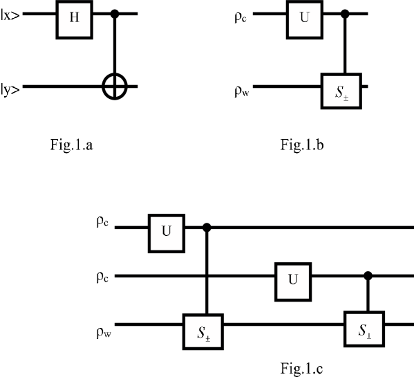
Figure 1: Fig.1 (a) Circuit generating entangled Bell states from product states using local Hadamard and non-local control-not gate; (b) Circuit generating the unitary evolution of the 1-step map $\varepsilon_{V}$ ; (c) Circuit generating entangled coin-walker states from corresponding factorized ones using local unitary (e.g Hadamard gate in the case of the homonymous QRW), and non-local control-control-$S_{\pm}$ gates, that form the map of the 2-step QRW $\varepsilon_{V}^{2}=\varepsilon_{W_{1}W_{2}}$.

Though the topic of the entanglement in the QRWs will not be investigated further here, it should be obvious from the above analysis that the CPTP map that implements some discrete time-step of a QRW, also generates quantum entanglement that can be studied by appropriate circuits and evaluated by effective measures, as usually is done in other cases of coupled quantum systems. Although quantum correlations have been generally accepted to be the common cause of all novel effects in the   QRW performance, the exact evaluation of the entanglement resources needed in the course of a QRW    is still an open problem.

To establish further the connection among ARQs and QRWs we give four particular examples:

i) the Euclidean QRW [13] [iso(2)-QRW]: with the distance operator $L\left|m\right\rangle=m\left|m\right\rangle,$ with its eigenspace $H_{w}^{L}=$span$\{\left|m\right\rangle,m\in\mathbf{Z}\}$, and its dual phase operator $\Phi\left|\varphi\right\rangle=\varphi\left|\varphi\right\rangle,$ with its eigenspace $H_{w}^{\Phi}=$span$\{\left|\varphi\right\rangle,\varphi\in[0,2\pi);\frac{d\varphi}{2\pi}\},$ related by a Fourier transform with $H_{w}^{L}.$ Two ARWs and its associated QRWs (modulo local unitary operators in coin spaces, as explained above), can be constructed: the distance random walk on $\mathbf{Z},$ with CPTP map constructed with Kraus generators been the step operators in the distance operator eigenstates i.e $\ S_{\pm}\left|m\right\rangle\equiv E_{\pm}\left|m\right\rangle=e^{\pm i\Phi}\left|m\right\rangle=\left|m\pm 1\right\rangle,$ and the phase random walk on the circle $S,$ with CPTP map constructed with Kraus generator been the step operators in the phase operator eigenstates i.e    $S_{\pm}\left|\varphi\right\rangle\equiv e^{\pm iL}\left|\varphi\pm 1\right\rangle;$

ii) the Canonical Algebra QRW [ hw-QRW]: with the position operator $Q\left|q\right\rangle=q\left|q\right\rangle,$ with its eigenspace $H_{w}^{Q}=$span$\{\left|q\right\rangle,q\in\mathbf{R};dq\},$ and its dual momentum operator $P\left|p\right\rangle=p\left|p\right\rangle,$ with its eigenspace $H_{w}^{P}=$span$\{\left|p\right\rangle,p\in\mathbf{R};dp\},$ related by a Fourier transform with $H_{w}^{Q}.$ Two ARWs and its associated QRWs (modulo local unitary operators in coin spaces, as explained above), can be constructed: the position random walk on $\mathbf{R},$ with CPTP map constructed with Kraus generators been the step operators in the position operator eigenstates i.e    $S_{\pm}\left|q\right\rangle\equiv e^{\pm iP}\left|q\right\rangle=\left|q\pm 1\right\rangle,$ and the momentum random walk on $\mathbf{R},$ with CPTP map constructed with Kraus generator been the step operators in the momentum operator eigenstates i.e    $S_{\pm}\left|p\right\rangle\equiv e^{\pm iQ}\left|p\right\rangle=\left|p\pm 1\right\rangle;$

iii) the $M-$ dimensional Discrete Heisenberg Group QRW [h_M-QRW]: with the action operator $N\left|n\right\rangle=n\left|n\right\rangle,$ with its eigenspace $H_{w}^{N}=$span$\{|n>,n\in\mathbf{Z}_{M}\},$ and its dual angle operator $\Theta\left|\vartheta_{n}\right\rangle=\vartheta_{n}\left|\vartheta_{n}\right\rangle,$ with its eigenspace $H_{w}^{\Theta}=$span$\{\left|\vartheta_{n}\right\rangle,$ $\vartheta_{n}\in\frac{1}{2\pi}\mathbf{Z}_{M}\},$ related by a finite Fourier transform with $H_{w}^{N}.$ Two ARWs and its associated QRWs (modulo local unitary operators in coin spaces, as explained above), can be constructed: the action random walk on $\mathbf{Z}_{M},$ with CPTP map constructed with Kraus generators been the step operators in the action operator eigenstates i.e    $\ S_{\pm}\left|n\right\rangle\equiv e^{\pm i\Theta}\left|n\right\rangle=h^{\pm 1}\left|n\right\rangle=\left|n\pm 1\right\rangle,$ and the angle random walk on $\frac{1}{2\pi}\mathbf{Z}_{M},$ with CPTP map constructed with Kraus generator been the step operators in the momentum operator eigenstates i.e    $S_{\pm}\left|\vartheta_{n}\right\rangle\equiv g^{\pm 1}\left|\vartheta_{n}\right\rangle=e^{\pm\not iN}\left|\vartheta_{n}\right\rangle=\left|\vartheta_{n\pm 1}\right\rangle;$

iv) the Coherent State QRW [15][ CS-QRW]: with the annihilation operator $a\left|\alpha\right\rangle=\alpha\left|\alpha\right\rangle,$ with its eigenspace $H_{w}^{a}=$span$\{\left|\alpha\right\rangle,\alpha\in\mathbf{C};\frac{d^{2}\alpha}{2\pi}\}.$Two ARWs and its associated QRWs (modulo local unitary operators in coin spaces, as explained above), can be constructed: the annihilation random walk on $\mathbf{C},$ with CPTP map constructed with Kraus generators been the step operators in the annihilation operator eigenstates i.e $\ S_{\pm}\left|\alpha\right\rangle\equiv e^{J(\pm 1)}\left|\alpha\right\rangle=D_{\pm 1}\left|\alpha\right\rangle=\left|\alpha\pm 1\right\rangle.$ The step operators here identified as special case of the canonical coherent state displacement operator $D_{\pm\beta}=e^{\pm\beta a^{\dagger}\mp\overline{\beta}a}=e^{J(\pm\beta)},$ have based the indicated step property on the following operator identity $D_{\alpha}D_{\beta}=e^{-i\alpha\times\beta}D_{\alpha+\beta},$ applied for the case of co-linear $\alpha,\beta$ vector on complex plane.

To give an explicit identification of the ARW based on the hw algebra constructed in [15], as a quantum random walk, and in particular as a CS-QRW, we make the following choices: the transition probabilities are $p_{+}=p,p_{-}=1-p$, the coin state is $\rho_{c}=|0><0|,$ the $U$ operator is $U(p,1-p)$, and the step operators are CS displacement operators with steps $\pm\beta\in\mathbf{C}.$ Then the total 1-step evolution operator in the coin+walker system is $V=\sum_{m=\pm}P_{m}U\otimes S_{m}=\left(\begin{array}[c]{cc}\sqrt{p}D_{+\beta}&\sqrt{1-p}D_{+\beta}\\ \sqrt{1-p}D_{-\beta}&-\sqrt{p}D_{-\beta}\end{array}\right),$ and the reduced walker evolves in 1-step by the CPTP $\varepsilon_{V}(\varrho_{w})=pD_{+\beta}\varrho_{w}D_{+\beta}^{\dagger}+(1-p)D_{-\beta}\varrho_{w}D_{-\beta}^{\dagger}=Tr_{c}(V\varrho_{c}\otimes\varrho_{w}V^{\dagger}).$

For $n$ steps the evolution of the walker has been chosen in [15] to be $\varepsilon_{V}^{n}(\varrho_{w}).$ It is important to notice that this is a choice based on the ARW construction methodology, and that our present treatment of the same walk as a QRW, sees the $\varepsilon_{V}^{n}(\varrho_{w})$ type of evolution to result from a partial tracing of the coin system at every step. Our previous discussion of other types of tracing schemes motivates the study of CS-QRWs with delayed tracing, in order to investigate phenomena such as enhanced or anomalous diffusion in ARWs. This problem will be taken up elsewhere.

5 Discussion

We have outlined a mathematical framework where the conception of random walk and its associated statistical notions, and equations of motion, can both be studied in an algebraic and quantum mechanical manner. ARWs and QRWs appear to be two aspects of the same mathematical device, so their interconnection serves to conceptually clarify the common ground between them and to enrich the heuristics of formulating new problems and methodically searching for their solutions.

Quantum random walks are important both as quantum algorithms to experimentally be realized and as modules in a general quantum computing algorithm-devise that could outperform some classical rival. The connection ARW-QRW could serve to generalize, unify and compare such algorithms.

Also Quantum Information Processing concepts and tools, could be developed for ARW-QRWs. The step taken here is only a preliminary one towards developing such a theory.

Finally, ARW-QRWs come with lots of free choices for its constituting parameters. To mention only one expected application in the field of Open Quantum Systems, we should emphasize the importance of choosing the functional in e.g the hw ARW. Various choices of functionals in terms of types of coherent state vectors, combined together with various choices of ordering the operator basis in the enveloping algebra $\mathcal{U}(\mathbf{hw})$, i.e normal, antinormal, symmetric etc, could serve as a guiding rule for constructing quantum master equations for open boson systems interacting with various types of quantum mechanical baths.

6 Acknowledgments

I wish to thank the organizers of the Volterra-CIRM-Grefswald Conference for the opportunity to give a talk. Discussions with L. Accardi, U. Franz, R. Hudson, M. Schürmann, and with my collaborators A. Bracken and I. Tsohantjis, are gratefully acknowledged. I am also grateful to the anonymous referee for suggesting eq.(63).

References

• [1] P. A. Meyer, Quantum Probability for Probabilists (Lect. Notes Math. 1538), (Springer, Berlin 1993).
• [2] M. Schürmann, White Noise on Bialgebras (Lect. Notes Math. 1544), (Springer, Berlin 1993).
• [3] S. Majid, Foundations of Quantum Groups Theory (Cambridge Univ. Press, 1955), ff. chapter 5.
• [4] U. Franz and R. Schott, Stochastic Processes and Operator Calculus on Quantum Groups, (Kluwer Academic Publishers, Dodrecht 1999).
• [5] A. Ambainis, E. Bach, A. Nayak, A. Vishwanath and J. Watrous, Proc. 33rd Annual Symp. Theory Computing (ACM Press, New York, 2001), p.37.
• [6] D. Aharonov, A. Ambainis, J. Kempe and U. Vasirani, Proc. 33rd Annual Symp. Theory Computing (ACM Press, New York, 2001), p.50.
• [7] A. Nayak and A. Vishwanath, arXive eprint quant-ph/0010117.
• [8] J. Kempe, Proc. 7th Int. Workshop, RANDOM’03, p.354 (2003).
• [9] A. M. Childs, E. Farhi and S. Gutmann, Quantum Information Processing 1, 35 (2002).
• [10] B. C. Travaglione and G. J. Milburn, Phys. Rev. A 65, 032310 (2002).
• [11] B. C. Sanders, S. D. Bartlett, B. Tregenna and P. L. Knight, Phys. Rev. A 67, 042305(2003).
• [12] J. Kempe, Contemp. Phys. 44, 307 (2003).
• [13] A. J. Bracken, D. Ellinas and I. Tsohantjis, J. Phys. A: Math. Gen. 37, L91(2004).
• [14] E. Abe, Hopf Algebras (CUP Cambridge 1997).
• [15] D. Ellinas, J. Comp. Appl. Math.133, 341 (2001).
• [16] A. W. Marshall and I. Olkin, Inequalities: Theory of Majorization and its Applications (Academic Press, New York, 1979).
• [17] R. Bhatia, Matrix Analysis (Spinger-Verlag, New York , 1997).
• [18] P. M. Alberti and A. Uhlmann, Stochasticity and Partial Order: Double Stochastic Maps and Unitary Mixing (Dordecht, Boston, 1982).
• [19] M. A. Nielsen, An Introduction to Majorization and its Applications to Quantum Mechanics (unpublished notes).
• [20] D. Ellinas and E. Floratos, J. Phys. A: Math. Gen. 32, L63 (1999).
• [21] B. D. Hughes, Random Walks and Random Environments Vol. I, (Clarendon Press, Oxford 1995)
• [22] J. Gillis, Quarterly J. Math., (Oxford, 2nd series)7, 144 (1956).
• [23] K. Lakatos-Lindenberg and K. E. Shuler, J. Math. Phys. 12, 633 (1971).
• [24] J. R. Klauder and B.-S. Skagerstam, Coherent States (World Scientific, Singapore (1986)
• [25] A. Perelomov, Generalized Coherent States and their Applications, (Springer - Verlag, Berlin 1986).
• [26] E. D. Davies, Quantum Theory of Open System, (Academic, New York, 1973).
• [27] G. Lindblad, Non-Equilibrium Entropy and Irreversibility, (Reidel, Dordrecht 1983).
• [28] M. O. Scully and  M. S. Zubairy, Quantum Optics, (Cambridge Univ. Press, Cambridge 1997), p. 255, 448, 453.
• [29] S. Stenholm, Phys. Scripta T12(1986).
• [30] J. Gea-Banacloche, Phys. Rev. Lett. 59, 543 (1987).
• [31] K. Kraus, States, effects and operations (Springer-Verlag, Berlin, 1983).
• [32] M. A. Nielsen and I. L. Chuang, Quantum Computation and Quantum Information, (Cambridge Univ. Press, Cambridge 2000).
• [33] S. Majid, Int. J. Mod. Phys. ${\bf 8}$ , 4521-4545 (1993).
• [34] S. Majid, M. J. Rodriguez-Plaza, J. Math. Phys. ${\bf 33}$, 3753-3760 (1994).
• [35] P. Feinsilver and R. Schott, J. Theor. Prob. 5, 251 (1992).
• [36] P. Feinsilver, U. Franz and R. Schott, J. Theor. Prob. 10, 797 (1997).
• [37] U. Franz and R. Schott, J. Phys. A: Gen . Math. 31 , 1395 (1998);
• [38] U. Franz and R. Schott, J. Math. Phys. 39, 2748 (1998).
• [39] D. Ellinas and I. Tsohantjis, J. Non-Lin. Math. Phys.8Suppl. 93(2001).
• [40] D. Ellinas and I. Tsohantjis,Inf. Dim. Anal.- Quant. Prob. 611 (2003).
• [41] G. H. Hardy, J. E. Littlewood and G. Polya, Messenger Math. 58, 145 (1929).
• [42] H. Sikic and M. V. Wickerhauser, Appl. Comp. Harm. Anal. 11, 147 (2001).
• [43] R. Gilmore, Lie Groups, Lie Algebras and Some of Their Applications, (Wiley, New York 1974).
• [44] D. Ellinas, et. al, work in progress.
• [45] P. J. Davis, Circulant Matrices, (Wiley, New York 1979).
• [46] M. R. Schroeder, Number Theory in Science and Communication, (Springer, Berlin 1997).
• [47] C. D. Cushen and R. L. Hudson, J. Appl. Prob. 8, 454 (1972).
• [48] This second line of the equation has the form a Lindblad type master equation taken in the large temperature limit, where for the average number of thermal photons we have $\overline{n}\approx\overline{n}+1=|\gamma|$, c.f.[28].
• [49] H. Risken, The Fokker-Planck Equation, (Springer, Berlin 1996). 83 (1990).