Heralded single-photon generation using imperfect single-photon sources and a two-photon-absorbing medium

Abstract

We propose a setup for a heralded, i.e. announced generation of a pure single-photon state given two imperfect sources whose outputs are represented by mixtures of the single-photon Fock state $|1\rangle$ with the vacuum $|0\rangle$. Our purification scheme uses beam splitters, photodetection and a two-photon-absorbing medium. The admixture of the vacuum is fully eliminated. We discuss two potential realizations of the scheme.

PACS numbers: 03.67.Lx, 42.50.Gy, 03.67.Hk

I Introduction

Light is an optimal candidate to be a carrier of quantum information because photonic states are durable due to the generally weak interaction with the environment. For this reason, the only realistic proposals for long distance quantum communication are still based on optical systems HNDP02 ; GCTC05 ; MRTZG03 . Photonic states are conveniently manipulated by means of linear optics and photodetection. However, most schemes to process photonic quantum information by means of linear optics require the ability to produce single photons. For example, the ingenious linear optics quantum computation scheme proposed by Knill, Laflamme and Milburn in KnillLaflammeMilburn2001 as well as the schemes for secure quantum communication in Bennett1984 ; Bennett1992 rely on the availability of single photons. Single photons entangled with the vacuum ($(|1\rangle|0\rangle+|0\rangle|1\rangle)/\sqrt{2}$) by a symmetric beam splitter can also be employed to teleport and transform single-rail optical qubits Babichev2001 ; Berry05 . Moreover, single-photon sources are a necessary resource in photonic quantum state engineering ScheelKnight2003 ; Welsch1999 ; Babichev2004 .

In recent years a variety of implementations for single photon sources has been investigated. Among them are schemes based on single molecule or atom excitation MoernerNJP04 ; AlleaumeNJP04 ; RempeNJP04 , single ions trapped in cavities WalterNJP04 , color centers in diamonds Weinfurter00 ; Grangier02 , quantum dots Yuan02 ; SantoriNJP04 and parametric down conversion (PDC) Fasel04 ; Pittman04 . These sources differ in the wavelength and purity of the emitted photons, their repetition rate and whether they produce a photon on demand or heralded, i.e, announced by an event. The latter is for example the case with PDC-sources. PDC produces randomly photon pairs and the presence of one photon is indicated by the detection of the other.

None of the existing single-photon sources, however, emits a pure single photon at a given time with certainty. The emission of multiple photons is negligible for most single-photon sources, cf. for example WalterNJP04 . Therefore their output in a certain mode can be modeled by a mixture of a single photon Fock state $|1\rangle$ and vacuum $|0\rangle$:

$$\rho=p|1\rangle\langle 1|+(1-p)|0\rangle\langle 0|\,,$$ (1)

where $p$ is called the efficiency of the single-photon source. Good sources have efficiencies of $p\approx 0.6$. To the best of our knowledge the highest efficiencies reached so far are $p=0.83$ Pittman04 and $p=0.86$ MoernerNJP04 .

In this article we propose a scheme to process two outputs from imperfect single photon sources (with efficiency $p<1$) in order to obtain a single photon with certainty ($p=1$) as desired for quantum information applications. These outputs may in fact originate from the same source. Using only linear optics and photodetection, it is impossible to produce a pure single photon with certainty by processing the outputs of imperfect sources. This is the case even if instead of two a finite number $n$ of imperfect sources are employed  BerryScheelSandersKnight2004 ; BerryScheelSandersKnightLaflamme2004 . Moreover, in order to obtain by means of linear optics a single photon with a probability $p<1$, which surpasses the efficiencies of the input sources, at least four such sources are needed. A corresponding scheme has been devised in BerryScheelSandersKnightLaflamme2004 at the expense of adding an additional multi-photon component to the output. Combining linear optics with homodyne detection seems not to improve the efficiency $p$. This has been shown at least for the case where only a single copy of the state $\rho$ as given in Eq. (1) is available Berry05 . These results suggest the usage of non-linear optical elements to improve the efficiency of imperfect single photon sources.

A possible solution to clean the single photon part in $\rho$ from the vacuum contribution (to build a “photon washer”) might be the usage of a quantum non-demolition measurement as proposed in Munro05 . In this article we follow a different road. Our proposal is based on a Mach-Zehnder interferometer, which contains a two-photon absorbing medium in one of its arms.

This article is organized as follows. The main part introduces our scheme (Sec. II) to generate pure single photons and shows how the improvement of the efficiency is accomplished (Sec. III). In Sec. IV we sketch settings where two-photon absorption might occur with sufficiently high probability to make the scheme feasible. In the appendix we discuss alternative realizations of single-photon generation without a Mach-Zehnder interferometer.

II The single-photon generator

Figure 1: $\rho_{1}$ and $\rho_{2}$ are imperfect single-photon states. They are superposed at a 50/50-beam-splitter $BS_{0}$. One of the resulting outputs is ignored (mode $A$) whereas the second one (mode $B$) is used as input of a Mach-Zehnder interferometer, which has a two-photon-absorbing medium ($TPAM$) in one of its arms. A successful generation of a single-photon Fock state $|1\rangle$ is indicated by a click of detector D₁ ($n_{B}=1$).

In this section we describe the setup and sketch the underlying physical ideas heuristically. The related calculations are then presented in the next section. Our setup is depicted in Fig. 1. The inputs $\rho_{1}$ and $\rho_{2}$ originate from two identical imperfect single-mode single-photon sources, with equal efficiency $p$: $\rho_{1}=\rho_{2}=p|1\rangle\langle 1|+(1-p)|0\rangle\langle 0|$, cf. Eq. (1). The first step of our scheme consists in superposing the two input states $\rho_{1}$ and $\rho_{2}$ at a beam splitter BS₀. One of the resulting outputs is discarded, whereas the other one is processed. The latter is used as input of a Mach-Zehnder interferometer with a two-photon absorbing medium ($TPAM$) in one of its arms. The interferometer is then followed by a photodetector D₁ which is required to click only in the case of a single photon. The detector measures one of the interferometer’s outputs, its second output contains the desired single-photon state $|1\rangle$ whenever a click in D₁ occurs.

The essential element of our arrangement is the two-photon-absorbing medium in one of the arms of the interferometer. Its action on the electromagnetic field in mode B is assumed to be given by

$$|0^{B}\rangle|g\rangle \xrightarrow{TPAM} |0^{B}\rangle|g\rangle$$

$$|1^{B}\rangle|g\rangle \xrightarrow{TPAM} |1^{B}\rangle|g\rangle$$

$$|2^{B}\rangle|g\rangle \xrightarrow{TPAM} \alpha|0^{B}\rangle|e\rangle+\beta|2^{B}\rangle|g\rangle\;.$$ (2)

In transformation (2) the first factor of the state represents the Fock state of mode B. The second factor refers to the collective quantum state of the medium. Here $|g\rangle$ denotes the “ground state” of the medium whereas the “excited state” $|e\rangle$ indicates that the medium has absorbed two photons. Please note, that it is not necessary in our context to further specify the collective excited state. Thus, only if two photons propagate through the $TPAM$ there is a non-vanishing probability $|\alpha|^{2}$ that both photons are absorbed. In case of one or zero photons in mode B no photon absorption takes place..

For $|\alpha|^{2}+|\beta|^{2}=1$ the $TPAM$ acts unitarily. To be more general we may also allow the $TPAM$ to induce a non-unitary transformation, describing, e.g., a unitary process followed by measurements. In the latter case $|\alpha|^{2}+|\beta|^{2}<1$. Later in this paper we will provide two possible realizations of the $TPAM$. One of them realizes a unitary $TPAM$ (see Sec. IV.1), while the second one implements a non-unitary $TPAM$ (see Sec. IV.2).

Note that two-photon absorption is possible whenever $\alpha\not=0$. In the limiting case $\alpha=0$ transformation (2) describes a non-linear phase-shift, if $\beta/|\beta|\not=1$: the phases of the states $|0\rangle|g\rangle$ and $|1\rangle|g\rangle$ are not altered whereas that of state $|2\rangle|g\rangle$ is changed. In general both effects, two-photon absorption and non-linear phase-shift are present. Nevertheless, in this paper we will refer to a medium causing transformation (2) as a two-photon absorbing medium ($TPAM$) regardless whether the latter or the former effect prevails.

Beam splitters BS₁ and BS₂ are chosen such that in the absence of the $TPAM$ detector D₁ cannot click, as a result of destructive interference within the interferometer. In this case the photons can leave the setup only in mode $C$. The mere existence of the interaction (2) leading to entanglement between the photons and the $TPAM$ destroys, partially, the interference of the two paths of the Mach-Zehnder interferometer. For two incoming photons the interference is disturbed maximally in case $|\alpha|=1$. In this latter case the $TPAM$ functions as a measuring apparatus performing a Null-measurement. Null-measurements are also called, in a slightly misleading way, “interaction-free measurements” Vaidman1993 ; Vaidman2003 . As a consequence, an event becomes possible which would be impossible in the absence of the $TPAM$, namely, the detection of a single photon at the detector D₁. Such a detection is possible only if two photons propagate through the interferometer. Thus, when detecting a single photon in D₁ we know on the one hand that two photons have been fed into the setup and on the other hand that they have not been absorbed by the $TPAM$. As a consequence, if conditioning on detection of a single photon in detector D₁, we can be sure that there is another single photon leaving the setup in mode $C$. A click of the detector D₁ announces the presence of a single photon in mode $C$. We thus have a heralded generation of a pure single-photon state in mode $C$.

III Theory

The calculations presented in this section reflect what has been said above. Let us start by providing the required transformations for a general beam splitter with two input modes $A_{1}$ and $A_{2}$ and two output modes $A^{\prime}_{1}$ and $A^{\prime}_{2}$ (cf. Fig. 2).

Figure 2: Beam splitter with two input modes $A_{1}$ and $A_{2}$ and two output modes $A^{\prime}_{1}$ and $A^{\prime}_{2}$.

For the purpose of this paper it is convenient to describe the action of the beam splitters in the Schrödinger picture. A pure input state can be written as $|\Psi\rangle=f(a^{\dagger}_{1},a^{\dagger}_{2})|0\rangle$. Here $a^{\dagger}_{1}$ and $a^{\dagger}_{2}$ are the creation operators corresponding to the field modes $A_{1}$ and $A_{2}$, and $f$ is some functional of them. In the same way we can represent the output state by $|\Psi^{\prime}\rangle=f^{\prime}(a^{\prime\dagger}_{1},a^{\prime\dagger}_{2})|0\rangle$, where the creation operators $a^{\prime\dagger}_{1}$, $a^{\prime\dagger}_{2}$ refer to the new field modes $A^{\prime}_{1}$ and $A^{\prime}_{2}$ and $f^{\prime}$ is some new functional. In order to obtain the output state $|\Psi^{\prime}\rangle$ from a given input state $|\Psi\rangle$ we have simply to perform the following formal replacements in $f(a^{\dagger}_{1},a^{\dagger}_{2})$ (cf. Scheel2003 ):

$$a_{1}^{\dagger} \rightarrow \tilde{a}^{\dagger}_{1}=\cos(\theta)a^{\prime{\dagger}}_{1}+e^{-i\phi}\sin(\theta)a^{\prime{\dagger}}_{2}$$

$$a_{2}^{\dagger} \rightarrow \tilde{a}^{\dagger}_{2}=-e^{i\phi}\sin(\theta)a^{\prime{\dagger}}_{1}+\cos(\theta)a^{\prime{\dagger}}_{2}\;,$$ (3)

i.e., $f^{\prime}(a^{\prime\dagger}_{1},a^{\prime\dagger}_{2})=f(\tilde{a}^{\dagger}_{1},\tilde{a}^{\dagger}_{2})$. For the sake of simplicity, however, in what follows below, we will denote the output field modes by the same letters omitting the prime labels, with a convention as already depicted in Fig.1. Note that the replacement transformation (3) should not be confused with the transformation of operators in the Heisenberg picture.

The initial input state reads:

$$\rho_{1}\otimes\rho_{2} = p^{2}|1^{A}1^{B}\rangle\langle 1^{A}1^{B}|+(1-p)(1-p)|0^{A}0^{B}\rangle\langle 0^{A}0^{B}|$$ (4)

$$+ (1-p)p|0^{A}1^{B}\rangle\langle 0^{A}1^{B}|+p(1-p)|1^{A}0^{B}\rangle\langle 1^{A}0^{B}|\,\,,$$

where the first and the second slot represent the number of photons in mode $A$ and mode $B$, respectively.

III.1 50/50-beam-splitters

We will see below that only the two-photon term of Eq. (4) is decisive, and that both photons have to be directed into mode $B$ by beam splitter BS₀. Starting with a general transformation (3) for BS₀ we calculate the density matrix which results for mode $B$ after applying BS₀ to the initial input state $\rho_{1}\otimes\rho_{2}$ and tracing out the discarded mode $A$:

$$\rho_{1}\otimes\rho_{2} \xrightarrow{\mbox{{\small Tr}}_{A}\,\circ\,\mbox{{\small BS}}_{0}}\,\rho_{B}= p^{2}\frac{\sin^{2}(2\theta_{0})}{2}|2\rangle\langle 2|+\left(p^{2}\cos^{2}(2\theta_{0})+p(1-p)\right)|1\rangle\langle 1|$$ (5)

$$+\left(p^{2}\frac{\sin^{2}(2\theta_{0})}{2}+(1-p)\right)|0\rangle\langle 0|\;.$$

Thus, the two-photon part is least diminished for $\theta_{0}=\frac{\pi}{4}$. It is therefore favorable to use a 50/50-splitter BS₀. In this case the density matrix in mode $B$ becomes

$$\rho_{B}=\frac{p^{2}}{2}|2\rangle\langle 2|+p(1-p)|1\rangle\langle 1|+\left(\frac{p^{2}}{2}-p+1\right)|0\rangle\langle 0|\;.$$ (6)

In order to make the calculation transparent we assume that also BS₁ and BS₂ are 50/50- beam splitters with $\phi=0$, cf. Fig. 1. The action of the beam splitters BS₁ and BS₂ on modes $B$ and $C$ is then given by:

$$b^{\dagger} \rightarrow \frac{1}{\sqrt{2}}\left(b^{\dagger}+c^{\dagger}\right)$$

$$c^{\dagger} \rightarrow \frac{1}{\sqrt{2}}\left(-b^{\dagger}+c^{\dagger}\right)\;.$$ (7)

Later in this section we will report that by employing more suitable beam splitters BS₁ and BS₂ the success probability for a heralded single-photon generation can be enhanced.

There are three possible pure input states that can enter the Mach-Zehnder interferometer in mode $B$. The corresponding probabilities appear in Eq. (6). We discuss the three alternative cases separately. The case of zero photons which occurs with probability $\mbox{prob}(0)=\left(\frac{p^{2}}{2}-p+1\right)$ trivially cannot be related with a click at the second single-photon detector D₁.

Let us now consider the case that exactly one photon is fed into the setup. It can come either from the input $\rho_{1}$ in mode A or from input $\rho_{2}$ in mode B. The over-all probability for a single photon being in mode $B$ amounts to $\mbox{prob}(1)=p(1-p)$. The photon interferes with the vacuum (in mode $C$) at the beam-splitter ${BS_{1}}$. In the following the first slot of the kets refers to mode $B$ and the second slot to mode $C$. The input state for the Mach-Zehnder interferometer is thus given by $|1^{B}0^{C}\rangle=b^{\dagger}|0^{B}0^{C}\rangle$. The calculations yield with Eqs. (2) and (7):

$$|1^{B}0^{C}\rangle=b^{\dagger}|0^{B}0^{C}\rangle \xrightarrow{BS_{1}} \frac{1}{\sqrt{2}}(b^{\dagger}+c^{\dagger})|0^{B}0^{C}\rangle$$ (8)

$$\xrightarrow{TPAM} \frac{1}{\sqrt{2}}(b^{\dagger}+c^{\dagger})|0^{B}0^{C}\rangle$$

$$\xrightarrow{BS_{2}} \frac{1}{\sqrt{2}}\left(\frac{1}{\sqrt{2}}(b^{\dagger}+c^{\dagger})+\frac{1}{\sqrt{2}}(-b^{\dagger}+c^{\dagger})\right)|0^{B}0^{C}\rangle$$

$$\xrightarrow{|1^{B}\rangle\langle 1^{B}|\otimes\openone^{C}} 0\;.$$

In the last line $|1^{B}\rangle\langle 1^{B}|\otimes\openone^{C}$ represents a projective selective measurement on mode $B$, the result being a detection of a single photon. Thus, just one photon entering the setup in mode $A$ or $B$ cannot cause a click in detector D₁.

What happens in the case in which two photons are fed into the setup, one in mode A and one in mode B? In the calculation below we will need to take into account also the state of the medium as soon as the measurement-like interaction inside the TPAM is applied. Furthermore, we will discard the mode which is detected. Again, the first slot of the kets refers to mode $B$ and the second slot to mode $C$, whereas the third slot represents the state of the medium. The input state for the Mach-Zehnder interferometer is now given by $|2^{B}0^{C}\rangle=\frac{1}{\sqrt{2}}(b^{\dagger})^{2}|0^{B}0^{C}\rangle$. Applying 50/50-beam-splitters BS₁ and BS₂, the $TPAM$, and conditioning on the detection of a single photon by detector D₁, yield:

$$|2^{B}0^{C}\rangle=\frac{1}{\sqrt{2}}(b^{\dagger})^{2}|0^{B}0^{C}\rangle \xrightarrow{BS_{1}} \frac{1}{2\sqrt{2}}(b^{\dagger}+c^{\dagger})^{2}|0^{B}0^{C}\rangle$$ (9)

$$=\frac{1}{2\sqrt{2}}(\sqrt{2}|2^{B}0^{C}\rangle+\sqrt{2}|0^{B}2^{C}\rangle+2|1^{B}1^{C}\rangle)$$

$$\xrightarrow{TPAM} \frac{1}{2\sqrt{2}}\Big{(}\phantom{\Big{)}}\sqrt{2}(\alpha|0^{B}0^{C}e\rangle+\beta|2^{B}0^{C}g\rangle)+$$

$$+\phantom{\Big{(}}\sqrt{2}|0^{B}2^{C}g\rangle+2|1^{B}1^{C}g\rangle\Big{)}$$

$$=\frac{1}{2\sqrt{2}}\Big{(}\phantom{\Big{)}}\sqrt{2}\alpha|0^{B}0^{C}e\rangle+\beta(b^{\dagger})^{2}|0^{B}0^{C}g\rangle+$$

$$+\phantom{\Big{(}}(c^{\dagger})^{2}|0^{B}0^{C}g\rangle+2b^{\dagger}c^{\dagger}|0^{B}0^{C}g\rangle\Big{)}$$

$$\xrightarrow{BS_{2}} \frac{1}{2\sqrt{2}}\Big{(}\beta\frac{1}{2}(b^{\dagger}+c^{\dagger})^{2}|0^{B}0^{C}g\rangle+\frac{1}{2}(-b^{\dagger}+c^{\dagger})^{2}|0^{B}0^{C}g\rangle\phantom{\Big{)}}$$

$$+\phantom{\Big{(}}(b^{\dagger}+c^{\dagger})(-b^{\dagger}+c^{\dagger})|0^{B}0^{C}g\rangle+\sqrt{2}\alpha|0^{B}0^{C}e\rangle\Big{)}$$

$$=\frac{1}{2\sqrt{2}}\bigg{(}\Big{(}\frac{1}{\sqrt{2}}(\beta+1)-\sqrt{2}\Big{)}|2^{B}0^{C}g\rangle+(\beta-1)|1^{B}1^{C}g\rangle\phantom{\Big{)}}$$

$$\phantom{\Big{(}}+\Big{(}\frac{1}{\sqrt{2}}(\beta+1)+\sqrt{2}\Big{)}|0^{B}2^{C}g\rangle+\sqrt{2}\alpha|0^{B}0^{C}e\rangle\bigg{)}$$

$$\xrightarrow{|1\rangle\langle 1|\otimes\openone\otimes\openone} \frac{1}{2\sqrt{2}}(\beta-1)|1^{C}g\rangle\;.$$

The final projective measurement by detector D₁ breaks the entanglement between the $TPAM$ and the photons. The $TPAM$ is transferred in a non-local way to the ground state $|g\rangle$.

The above calculation shows that, whenever two photons are fed into the setup there is a non-vanishing probability for a click event at the final detector D₁. Moreover, on the condition of this event one can be sure that another single photon is leaving our device in mode $C$. A detection of a single photon by detector D₁ guarantees a perfect preparation of a single photon Fock state $|1\rangle$ in mode $C$. The probability for a click in detector D₁, given that two photons are injected into the Mach-Zehnder interferometer in mode $B$, amounts to $\frac{1}{8}|1-\beta|^{2}$, as can be inferred from the norm of the resulting (unnormalized) final quantum state. With the probability for two photons entering the Mach-Zehnder interferometer in mode $B$ being $\mbox{prob}(2)=p^{2}/2$ (cf. Eq.(6)), the over-all probability for success thus amounts to

$$P^{50/50}_{\mbox{\scriptsize s}}=\frac{1}{16}|1-\beta|^{2}p^{2}\;.$$ (10)

III.2 The general case

The success probability $P_{\mbox{\scriptsize s}}$ can be increased by employing more suitable beam splitters BS₁ and BS₂. This follows from an analysis of the scheme using general beam-splitter transformations (3) for BS₁ and BS₂. We omit the details of the calculations.

The requirement that a single photon entering the setup either in mode $A$ or in mode $B$ must not cause a click in the detector D₁ restricts the possible values of the beam-splitter parameters $\phi_{1},\phi_{2},\theta_{1},\theta_{2}$. This requirement firstly implies that $(\phi_{1}-\phi_{2})=\nu\pi$ with $\nu\in\mathbb{Z}$. The conditions for $\theta_{1}$ and $\theta_{2}$ depend on whether $(\phi_{1}-\phi_{2})=\nu(2\pi)$ or $(\phi_{1}-\phi_{2})=(2\nu+1)\pi$, with $\nu\in\mathbb{Z}$. In the first case we must have $(\theta_{1}+\theta_{2})=\pm\frac{\pi}{2}$, while in the second case we must choose $\theta_{1}$ and $\theta_{2}$ such that $(\theta_{1}-\theta_{2})=\pm\frac{\pi}{2}$. Taking into account these conditions we obtain the following: If we choose $(\phi_{1}-\phi_{2})=\nu(2\pi)$ and $(\theta_{1}+\theta_{2})=+\frac{\pi}{2}$ or $(\phi_{1}-\phi_{2})=(2\nu+1)\pi$ and $(\theta_{1}-\theta_{2})=+\frac{\pi}{2}$, the calculation yields

$$P_{\mbox{\scriptsize s}}(\beta,\theta_{1},\theta_{2})=p^{2}|1-\beta|^{2}\cos^{6}(\theta_{1})\sin^{2}(\theta_{1})\;,$$ (11)

whereas the choices $(\phi_{1}-\phi_{2})=\nu(2\pi)$ and $(\theta_{1}+\theta_{2})=-\frac{\pi}{2}$ or $(\phi_{1}-\phi_{2})=(2\nu+1)\pi$ and $(\theta_{1}-\theta_{2})=-\frac{\pi}{2}$ lead to

$$P_{\mbox{\scriptsize s}}(\beta,\theta_{1},\theta_{2})=p^{2}|1-\beta|^{2}\sin^{6}(\theta_{1})\cos^{2}(\theta_{1})\;.$$ (12)

Please note, that the optimal reflectivity of BS₁ and BS₂ does not depend on the parameters characterizing the $TPAM$.

The success probability becomes maximal for $\theta_{1}^{\mbox{\scriptsize max}}=30^{\circ},150^{\circ},210^{\circ},330^{\circ}$ in the first case (11) and for $\theta_{1}^{\mbox{\scriptsize max}}=60^{\circ},120^{\circ},240^{\circ},300^{\circ}$ in the second case (12). The most suitable beam splitters thus turn out to be a $BS_{1}$ with reflectivity of $3/4$ and a BS₂ with reflectivity of $1/4$, or vice versa. In addition the phase condition $(\phi_{1}-\phi_{2})=\nu\pi$ has to be fulfilled. The maximal success probability that can be reached by variation of the beam-splitter parameters, is

$$P^{\mbox{\scriptsize max}}_{\mbox{\scriptsize s}}(\beta)\equiv P_{\mbox{\scriptsize s}}(\beta,\theta^{\mbox{\scriptsize max}}_{1},\theta^{\mbox{\scriptsize max}}_{2})=\frac{27}{256}p^{2}|1-\beta|^{2}\approx 0.1055\times p^{2}|1-\beta|^{2}\;.$$ (13)

It still depends on $\beta$, which characterizes the action of the $TPAM$, cf. Eq. 2. $P^{\mbox{\scriptsize max}}_{\mbox{\scriptsize s}}(\beta)$ becomes zero, if there is no $TPAM$ in one of the interferometer arms, i.e., in case $\beta=1$. $P^{\mbox{\scriptsize max}}_{\mbox{\scriptsize s}}(\beta)$ becomes maximal for $\beta=-1$, which means no two-photon absorption but just a non-linear phase shift. In the latter case a success probability $P^{\mbox{\scriptsize max}}_{\mbox{\scriptsize s}}(\beta=-1)\approx 0.4219\times p^{2}$ is attained. Note, that to alter the phase of $\beta$ by introducing a global phase factor in the third transformation rule of (2) would entail the introduction of the same phase factor in the first two transformation rules of (2). The calculations show that probability $P^{\mbox{\scriptsize max}}_{\mbox{\scriptsize s}}(\beta)$ is left invariant, as it is expected, under such a global phase change. In the next section we consider realizations of $TPAM$s with real positive values for $\beta$. In this case $P^{\mbox{\scriptsize max}}_{\mbox{\scriptsize s}}(\beta)$ increases with growing two-photon absorption rate. It assumes its maximal value $P^{\mbox{\scriptsize max}}_{\mbox{\scriptsize s}}=\frac{27}{256}p^{2}$ for $|\alpha|=1$ or $\beta=0$, respectively.

Figure 3: Enhancement of the success probability by a factor of 2 by processing both outputs of BS₀ using identical interferometers with a $TPAM$ and final detectors D₁ — instead of discarding one of them as done in the original setup (cf.  Fig. 1).

A further enhancement of the success probability by a factor of 2 can be achieved by processing the second output of BS₀ in the same way as the first one (cf. Fig. 3), instead of discarding it. The second output is directed into an identical interferometer with a $TPAM$ and a final detector D₁. Provided that two ingoing photons take the upper way this alternative heralds a pure single photon with the same probability as in the lower case. Since both photons choose either the upper or the lower path with equal probability — due to the Hong-Ou-Mandel effect — the two alternatives are exclusive. Therefore the corresponding success probabilities for heralding a photon are additive. As a result, the over-all maximum success probability that can in principle be achieved with such an extension of our scheme amounts to $2\times P^{\mbox{\scriptsize max}}_{\mbox{\scriptsize s}}(\beta=-1)=2\times 4\times\frac{27}{256}p^{2}=0.84375\times p^{2}$. This is remarkably high as compared to the upper bound $p^{2}$ of the probability for a heralded generation of a single photon from two identical sources with efficiency $p$.

IV Realization

We believe that the scheme proposed above is interesting in its own right. Whether our method to generate a single photon from two imperfect sources can already be applied in a laboratory depends on the availability of a setup which realizes state transformation (2), such that the success probability $P_{\mbox{\scriptsize s}}\propto|1-\beta|^{2}$ is sufficiently high. In the following we are going to suggest two candidates for the implementation of state transformation (2). We will refer to each of them as two-photon absorbing medium (TPAM), even though they rather resemble machines built out of several units. Both TPAMs use special settings to amplify two-photon absorption, which normally is a much weaker effect than absorption or scattering of a single photon. These settings stem from different contexts. We propose modifications which make them suitable for our purpose.

IV.1 TPAM realized by a thin hollow optical fiber containing three-level atoms

A TPAM is realized whenever the medium can absorb two photons, whereas just one photon is not absorbed. A good model for understanding two-photon absorption is given by three-level atoms (cf. FransonJacobsPittman2004 ). Fig. 4 illustrates how two-photon absorption can take place, while single-photon absorption is impossible due to detuning.

Figure 4: Illustration of two-photon absorption by means of three-level atoms (cf. FransonJacobsPittman2004 ). The atomic levels are labeled by 1, 2 and 3 while the photons are indicated by their wave numbers $k$. In (a) a single photon can be absorbed. This is avoided by detuning (b).

Two-photon absorption is a nonlinear effect and is therefore commonly expected to be small for intensities corresponding to a few photons only. A way to amplify this nonlinear process is to insert three-level atoms with appropriate detuning into a thin hollow optical fiber. Such a proposal has recently been discussed by Franson et al. in FransonJacobsPittman2004 in the context of optical realizations of quantum gates. There it is argued that the confinement of a single-photon wave packet within a very narrow optical fiber involves concentration of the photon energy into a very small volume. The confinement can thus produce relatively large electric fields which in turn entail the possibility of large nonlinearities, including two-photon absorption. According to estimates provided in FransonJacobsPittman2004 it is feasible to achieve two-photon absorption rates in optical fibers that correspond to a two-photon absorption length on the order of $5m$. Given that such values can in fact be achieved, we believe that $|\alpha|$-values (cf. Eqs. 2) close to $1$ are feasible. Since in this realization of the $TPAM$ no measurements take place, the transformation (2) is unitary and therefore we have $|\beta|^{2}=1-|\alpha|^{2}\approx 0$ for high two-photon absorption rates, which involves a success probability $P^{\mbox{\scriptsize max}}_{\mbox{\scriptsize s}}(\beta\approx 0)\approx\frac{27}{256}p^{2}\approx 0.1055\times p^{2}$.

Certain losses need to be overcome that might cause failure events of such a realization of the single-photon generator. The main technical challenge seems to consist in suppressing the single-photon scattering which, under most conditions, is expected to prevail the two-photon absorption. However, scattering of a single photon into another mode is suppressed due to the fact that only the propagation of a certain mode is supported within a single-mode optical fiber. The mere fact that quantum key distribution is possible, which relies on the feasibility to transmit single photons through several kilometers of optical fibers, is a strong evidence that losses due to single-photon scattering can be made negligible.

Additional losses might be caused when coupling the photons into the optical fiber. This problem can be circumvented by using imperfect single photon sources that provide photons inside a single-mode optical fiber at the outset. Such imperfect single photon sources have been reported on, e.g., in Fasel04 ; Pittman04 . Moreover, it is experimentally feasible to realize beam splitters and phase shifters by means of optical fibers (see e.g. Fasel04 ; Pittman04 ). Thus, our setup of Sec. II can be built in such a way that all processes apart from the final detection take place within optical fibers. We believe that all these problems can be tackled so as to make our proposal of Sec. II and III promising.

IV.2 TPAM using resonant nonlinear optics and time selection

In this section we introduce another method to realize a two-photon absorbing medium (TPAM), which we refer to as “time selection”. We first outline the principle. Then we describe a setup with non-linear optics proposed by Johnsson and Fleischhauer JohnssonFleischhauer2003 and modify it to realize a TPAM based on time selection.

The $TPAM$ in our scheme has the task to only absorb a pair of photons while being transparent for a single photon. The obvious way to tackle this task is by means of energy selection. That is to choose a medium whose transition energy is on resonance with the energy of two photons but not with the energy of a single photon. The required two photon process is a second order effect and has to be enhanced by a special setting to occur with a reasonable probability. The setup described in the previous section goes along these lines by confining the electromagnetic field in an optical fiber. We now turn to a different scheme.

An alternative to energy selection might be “time selection”, which will be explained in the following. Let us assume that the state of light in the medium traverses a cycle with a period which depends on the initial number of photons. The length of the medium can then be adjusted to the time $T_{1}$ it takes for a single photon state to reoccur

$$|1\rangle|g\rangle\xrightarrow{U(T_{1})}|1\rangle|g\rangle\,.$$ (14)

Here $|g\rangle$ represents the initial state (ground state) of the medium. Two photons run through a different cycle with period $T_{2}\not=T_{1}$ and emerge after time $T_{1}$ from the medium in an entangled state

$$|2\rangle|g\rangle\xrightarrow{U(T_{1})}\alpha_{0}|0\rangle|e_{2}\rangle+\alpha_{1}|1\rangle|e_{1}\rangle+\beta|2\rangle|g\rangle\,,$$ (15)

where $|e_{1}\rangle$ and $|e_{2}\rangle$ are excited states of the medium corresponding to one and two absorbed photons, respectively. If zero photons enter the medium, then also zero photons will emerge form it:

$$|0\rangle|g\rangle\xrightarrow{U(T_{1})}|0\rangle|g\rangle\,.$$ (16)

Eqs. (14), (15) and (16) already resemble the state transformation (2) required for the TPAM apart from the one photon term in Eq.  (15). This term has to be eliminated because a one photon contribution after the TPAM could trigger detector $D_{1}$ leaving vacuum in the output of our single photon generator (cf. Fig. 1). One method to remove the one photon contribution in Eq.  (15) would be a conditional measurement projecting on a subspace orthogonal to state $|e_{1}\rangle$. For this purpose, however, the corresponding degree of freedom of the medium has to be accessible by measurement.

Johnsson and Fleischhauer (JF) JohnssonFleischhauer2003 proposed a setup using resonant four-wave mixing with two pump fields $\Omega_{1}$, $\Omega_{2}$ and two generated fields $E_{1}$, $E_{2}$, where the energy cycles between the pump- and the generated fields. In their scheme the light fields interact via a vapor of five-level atoms (see Fig. 5) which can be understood as modified double $\Lambda$-systems. The additional level $|3\rangle$ serves to compensate non-linear phase shifts of the light fields, which would prevent energy cycling with unit efficiency. The modification also reduces the period of the cycle as compared to a generic double-$\Lambda$ system JohnssonFleischhauer2002 . Initially the atom is in state $|1\rangle$ and the first pump field $\Omega_{1}$ contains $n$ photons. The light fields $E_{1}$ and $E_{2}$ are initially not excited but generated by the interaction of light and matter. The second pump field $\Omega_{2}$ consists of a strong coherent cw input which enhances the cycling. All fields propagate in the same direction. Choosing a driving field $\Omega_{1}$ in resonance with the $|2\rangle-|5\rangle$ transition and a driving field $\Omega_{2}$ with detuning $\mp\Delta$ with respect to the $|1\rangle-|3\rangle,|4\rangle$ transition, minimizes losses due to single photon absorption. It can be shown that the fields $E_{1}$ and $E_{2}$ are then generated precisely with frequencies, such that there are two-photon resonances from the pair $\Omega_{1}$, $E_{1}$ and from the pair $\Omega_{2}$, $E_{2}$ corresponding to $|1\rangle-|2\rangle$ transitions. This results in an overall four-photon resonance.

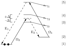
Figure 5: Four-wave mixing scheme in a modified double-$\Lambda$ system according to Johnsson and Fleischhauer JohnssonFleischhauer2003 . In order to avoid non-linear phase shifts, $d_{42}d_{41}d_{32}d_{31}<0$, where $d_{ij}=\langle i|d|j\rangle$ is the matrix element of the dipole moment corresponding to the $|i\rangle-|j\rangle$ transition. $\gamma_{1},\gamma_{2},\gamma_{3}$ indicate spontaneous decay rates of the corresponding energy levels. The level scheme is realized in the hyperfine structure of atoms JohnssonFleischhauer2002 .

According to the results of JF JohnssonFleischhauer2003 the evolution of the initial state $|\psi(0)\rangle=|1,0,0\rangle$ is given by

$$|\psi(t)\rangle=\cos(\kappa|\Omega_{2}|ct)|1,0,0\rangle-i\sin((\kappa|\Omega_{2}|ct)|0,1,1\rangle\,,$$ (17)

where $|l,m,n\rangle$ represents the Fock state with $l,m$ and $n$ photons in the modes corresponding to the fields $\Omega_{1}$, $E_{1}$ and $E_{2}$, respectively. The coherent cw field $\Omega_{2}$ can be treated classically. Here $\kappa:=3N\lambda^{2}\gamma/(8\pi\Delta)$ and $N$ is the atomic number density, $\lambda$ and $\gamma$ are some typical wavelength and radiative decay rate, respectively (cf. JohnssonFleischhauer2003 ). Eq. (17) indicates an oscillation between states with one photon in $\Omega_{1}$ and one photon in $E_{1}$ and $E_{2}$ each. Following the scheme of JF we restrict the length of the nonlinear medium to a multiple $M$ of $L_{0}=\pi/(\kappa|\Omega_{2}|)$. A medium with such a length will be transparent for a single photon in $\Omega_{1}$:

$$|1,0,0\rangle\xrightarrow{U(t=ML_{0}/c)}(-1)^{M}|1,0,0\rangle\;,$$ (18)

except for a phase shift for odd $M$, which can be compensated for by an additional phase shifter. This corresponds to the method of “time selection” mentioned above, cf. Eq. (14). But here the role of the state of the medium $|g\rangle$ in Eq. (14) is played by the state of the radiation fields $E_{1}$, $E_{2}$. This is advantageous since this state is accessible by measurement.

Starting with two photons in $\Omega_{1}$, i.e.  $|\psi(0)\rangle=|2,0,0\rangle$, one obtains the following state after time $t=ML_{0}/c$:

$$|2,0,0\rangle\xrightarrow{U(t=ML_{0}/c)}\alpha_{0}|0,2,2\rangle+\alpha_{1}|1,1,1\rangle+\beta|2,0,0\rangle\,.$$ (19)

The values of $\alpha_{0}$, $\alpha_{1}$ and $\beta$ as functions of the interaction time are given by (cf.  JohnssonFleischhauer2003 )

$$\alpha_{0}(t)=-\dfrac{2\sqrt{2}}{3}\dfrac{\Omega_{2}}{\Omega_{2}^{*}}\sin^{2}\left(\frac{\varphi(t)}{2}\right)\quad \alpha_{1}(t)=-\frac{i}{\sqrt{3}}\sqrt{\frac{\Omega_{2}}{\Omega_{2}^{*}}}\sin\left(\varphi(t)\right)$$ (20)

$$\beta(t)=\dfrac{1}{3}\left[2+\cos\left(\varphi(t)\right)\right]\quad \mbox{with}\quad\varphi(t):=\sqrt{\frac{3}{2}}\kappa|\Omega_{2}|ct\,.$$

Now the second term in Eq. (19) represents a one photon contribution and has to be eliminated to yield a state transformation of form (2), which realizes the TPAM. This can be done by detecting the photons of the generated fields $E_{1}$ and $E_{2}$. The proposal of JF also contains such a detection. They assume a beam splitter which transmits the pump fields $\Omega_{i}$ and reflects the generated fields $E_{i}$ ($\,i=1,2$), followed by a detector for the $E_{i}$ (cf. BS₄ of Fig.6). Such a beam splitter can, e.g., be realized by choosing orthogonal polarizations for the $\Omega_{i}$ and the $E_{i}$ and using a polarizing beam splitter. Alternatively a system of dichroic beam splitters could be employed, which transmit or reflect light depending on its wavelength.

Figure 6: Implementation of the four-wave mixing scheme. $\Omega_{1}$ is identical with mode B of the Mach-Zehnder interferometer in Fig. 1

At this point we deviate from the proposal of JF. They consider a sequence of nonlinear media with length $L_{0}$ and detectors which makes the state of the radiation field converge to a mixture of $|1,0,0\rangle$ and vacuum with probability one. Our objective, however, is to eliminate the vacuum contribution and obtain a single-photon state. For this purpose we suggest to condition on the detection of zero photons in $E_{1}$ and $E_{2}$. This leads to the following state transformation

$$|2,0,0\rangle\xrightarrow{\left(\openone\otimes|0\rangle\langle 0|\otimes|0\rangle\langle 0|\right)\,U(t=L_{0}/c)}\beta|2,0,0\rangle$$ (21)

with $\beta=0.4130$. With this result a special instance of the desired transformation (2) is established and the TPAM comprising the vapor of five-level atoms, the driving field $\Omega_{2}$ and a detector $D$ can be implemented in one arm of the Mach-Zehnder interferometer (cf. Fig. 1) as shown in Fig. 6. The coherent cw field $\Omega_{2}$ generated by a laser is superposed with $\Omega_{1}$ (Mode B of the Mach-Zehnder interferometer in Fig. 1) by means of a dichroic beam splitter. At the end of the TPAM the cw-field $\Omega_{2}$ has to be filtered out by means of a frequency filter. The value of $\beta$ in transformation (21) leads to a success probability of $P_{\mbox{\scriptsize s}}\approx 0.0363\times p^{2}$ for the generation of a single photon. Please note, that due to the fact that $\varphi(t=ML_{0}/c)=M\pi\sqrt{3/2}$ in $\beta$ as given by (20) is an irrational multiple of $\pi$, any value of $\varphi\in[0,2\pi]$ is assumed with arbitrary accuracy when choosing $M$, i.e., the length of the medium, appropriately. The success probability $P_{\mbox{\scriptsize s}}$ can in principle be increased up to the value $P_{\mbox{\scriptsize s}}^{\mbox{\scriptsize max}}\approx 0.0469\times p^{2}$ for $\beta=\frac{1}{3}$. Already for a medium of length $4L_{0}$ a success probability of $P_{\mbox{\scriptsize s}}\approx 0.0446\times p^{2}$ is accomplished.

The JF setup can thus be modified and employed as TPAM within our scheme in order to generate single-photon Fock states from two outputs of imperfect single photon sources. But this is not the only way to accomplish this task. In the appendix we sketch two alternative schemes without Mach-Zehnder interferometer to remove the vacuum contribution, which is still present in the output of original JF setup.

V Conclusion

The scheme to generate single photons as proposed in sections 1 and 2 is clear cut and simple from a conceptual point of view. It also allows to generate a single photon heralded by a click of detector $D_{1}$ with an efficiency of $100\%$ from two single-photon sources with any efficiency $1>p>0$. In principle, our proposal allows for a success probability $P_{\mbox{\scriptsize s}}\approx 0.84\times p^{2}$. However, whether it is experimentally applicable, e.g. in a quantum computation or a quantum cryptography protocol which relies on single photons, depends essentially on the existence of a medium or a machine which implements the state transformation given in Eq. (2) and gives rise to a sufficiently high success probability $P_{\mbox{\scriptsize s}}\propto|1-\beta|^{2}$. We propose two candidates to realize this transformation.

The first employs three-level atoms which can only absorb a pair of photons because of energy conservation. They are enclosed in an optical fiber for two reasons. Firstly, confining the electromagnetic field in the fiber increases the energy density and thus enhances non-linear effects such as two-photon absorption. Secondly the optical fiber may carry only certain modes and hence suppresses scattering of single photons. A fiber of approximately. $5m$ length yields a sufficiently high probability for two photon absorption.

The second candidate employs resonant four-wave mixing in a vapor of five-level atoms with a strong coherent cw driving field $\Omega_{2}$ in addition to the incident light field $\Omega_{1}$ from the imperfect sources. Due to the four-wave mixing two additional light fields $E_{1}$ and $E_{2}$ are generated and the energy cycles between the four fields. The period depends on the number of photons $\Omega_{1}$ initially contains. The length of the medium is adjusted such that a single photon in $\Omega_{1}$ leaves the atomic vapor unchanged while two photons are entangled with the generated fields $E_{1}$ and $E_{2}$. A conditioned measurement of the number of photons in $E_{1}$ and $E_{2}$ realizes state transformation (2) leading to reasonably high success probabilities $P_{\mbox{\scriptsize s}}$.

Acknowledgment: We would like to thank Alex Lvovsky, Lajos Diosi, Christian Kasztelan, Rudolf Bratschitsch, Florian Adler, and Matthias Kahl for helpful discussions. This work was supported by the “Center for Applied Photonics” (CAP) at the University of Konstanz.

Appendix: Single-photon generation without Mach-Zehnder interferometer

We found two alternative modifications of the setup of Fleischhauer and Johnsson (see Sec. IV.2) to generate a pure single-photon state out of two noisy photon states $\rho_{1}=\rho_{2}=p|1\rangle\langle 1|+(1-p)|0\rangle\langle 0|$. Both schemes deviate from the mechanism described in Sec. II and III, since they operate without a Mach-Zehnder interferometer. They are depicted in Figs. 7 and 8. The alternative schemes use as central unit the implementation of the TPAM by four-wave mixing which is described above (cp. Fig.  6). The input field $\Omega_{1}$ of the TPAM consists of the mixture (6) gained from superposing state $\rho_{1}$ and $\rho_{2}$ at a symmetric beam splitter BS₀.

Figure 7: Alternative setup based on the scheme of JF with nonlinear medium (vapor) of length $L_{1}=2L_{0}$. Detector D₁ is conditioned on 1 photon in $E_{1}$ and $E_{2}$ each. The success probability amounts to $P_{\mbox{\scriptsize s}}\approx 0.1620\times p^{2}$

The first alternative uses a vapor of length $L_{1}=2L_{0}$ with $L_{0}=\frac{\pi}{\kappa|\Omega_{2}|}$ corresponding to a full cycle of a single incident photon in $\Omega_{1}$, cf. Eq. (17):

$$|0,0,0\rangle\xrightarrow{U(t=L_{1}/c)}|0,0,0\rangle\;,$$

$$|1,0,0\rangle\xrightarrow{U(t=L_{1}/c)}|1,0,0\rangle\;,$$

$$|2,0,0\rangle\xrightarrow{U(t=L_{1}/c)}\alpha_{0}^{(L_{1})}|0,2,2\rangle+\alpha_{1}^{(L_{1})}|1,1,1\rangle+\beta^{(L_{1})}|2,0,0\rangle\,.$$ (22)

Conditioning on the detection of one photon in $E_{1}$ and $E_{2}$, respectively, eliminates the contributions from a single incident photon and vacuum in $\Omega_{1}$ while it selects the single-photon contribution from two incident photons. Thus the over-all state change of the scheme depicted in Fig. 7 amounts to

$$\rho_{1}\otimes\rho_{2}\rightarrow\frac{p^{2}|\alpha_{1}^{(L_{1})}|^{2}}{2}|1\rangle\langle 1|$$ (23)

This process occurs with probability $P_{\mbox{\scriptsize s}}=p^{2}|\alpha_{1}^{(L_{1})}|^{2}/2\approx 0.1620\times p^{2}$, cf. (20). The maximum success probability, achievable by choosing suitable multiples of length $L_{0}$, is given by $P_{\mbox{\scriptsize s}}^{\mbox{\scriptsize max}}\approx 0.1667\times p^{2}$.

Figure 8: Setup with nonlinear medium (vapor) of length $L_{2}=2L_{0}/3$. Detector $D_{1}$ is conditioned on zero photons in $E_{1}$ and $E_{2}$. The success probability is $P_{\mbox{\scriptsize s}}\approx 0.2291\times p^{2}$.

The second alternative to prepare the single-photon state $|1\rangle$ using the JF-setup is sketched in Fig. 8. This time the length of the medium (vapor) is given by $L_{2}=3L_{0}/2$, which induces the state change

$$|0,0,0\rangle\xrightarrow{U(t=L_{2}/c)}|0,0,0\rangle\;,$$

$$|1,0,0\rangle\xrightarrow{U(t=L_{2}/c)}i|0,1,1\rangle\;,$$

$$|2,0,0\rangle\xrightarrow{U(t=L_{2}/c)}\alpha_{0}^{(L_{2})}|0,2,2\rangle+\alpha_{1}^{(L_{2})}|1,1,1\rangle+\beta^{(L_{2})}|2,0,0\rangle\,.$$ (24)

After detection of zero photons in detector D₁ (cf. Fig. 8), $\Omega_{1}$ either contains zero or two photons. Detecting one photon in one of the outputs of a subsequent symmetric beam splitter indicates one photon in the other output. These measurement outcomes and thus the single photon generation occurs with probability $P_{\mbox{\scriptsize s}}=p^{2}|\beta^{(L_{2})}|^{2}/4\approx 0.2291\times p^{2}$. By varying $M\in\mathbb{N}$ in $L_{2}=(2M-1)L_{0}/2$ one can achieve $P_{\mbox{\scriptsize s}}^{\mbox{\scriptsize max}}=0.25\times p^{2}$.

The latter implementation generates a single photon with higher probability, but it requires an additional detector. The two alternatives possess higher success probabilities than the implementation of our original scheme by means of the JF-mechanism ($P_{\mbox{\scriptsize s}}\approx 0.0234$). However, the alternative devices depend on the feasibility of the JF-mechanism, while our original scheme may be realized in many ways, i.e., by employing different TPAMs. Moreover, our original scheme as described in Sections II and III can, in principle, yield higher success probabilities. Please note that the success probabilities mentioned above can be doubled by processing the second output of BS₀ in the very same manner as the first output (cf. to  Sec. III).

References

- (1) R. J. Hughes, J. E. Nordholt, D. Derkacs and C. G. Peterson, New J. Phys. 4 (2002).
- (2) K. J. Gordon, R. J. Collins, P. D. Townsend, S. D. Cova, Proceedings of SPIE, 2005.
- (3) I. Marcikic, H. de Riedmatten, W. Tittel, H. Zbinden and N. Gisin, Nature 421, 509-513 (2003).
- (4) E. Knill, R. Laflamme and G. J. Milburn, Nature 409, 46 (2001).
- (5) C.H. Bennett and G. Brassard, in Proc. IEEE Int. Conf. on Computers, Systems and Signal Processing, (Bangalore, India) (New York: IEEE), 1984.
- (6) C.H. Bennett, G. Brassard, and A. Ekert, Sci. Am. 267, 50 (1992).
- (7) S. A. Babichev, J. Ries and A. I. Lvovsky, Europhys. Lett. 64 (1) , pp. 1-7 (2003).
- (8) D. W. Berry, A. I. Lvovsky, B. C. Sanders, preprint: quant-ph/0507216, 2005.
- (9) S. Scheel, K. Nemoto, W. J. Munro, and P. L. Knight, Phys. Rev. A 68, 032310 (2003).
- (10) J. Clausen, M. Dakna, L. Knöll, and D.-G. Welsch, Acta Phys. Slov. 49, 653 (1999).
- (11) S. A. Babichev, B. Brezger, and A. I. Lvovsky, Phys. Rev. Lett. 92, 047903 (2004).
- (12) W. E. Moerner, New J. Phys. 6, 88 (July 2004).
- (13) R. Alléaume, F. Treussart, J. M. Courty and J. F. Roch, New J. Phys. 6, 85 (2004).
- (14) M. Hennrich, T. Legero, A. Kuhn and G. Rempe, New J. Phys. 6 (July 2004).
- (15) M. Keller, B. Lange, K. Hayasaka, W. Lange and H. Walther, New J. Phys. 6, 95 (July 2004).
- (16) C. Kurtsiefer, S. Mayer, P. Zarda, and H. Weinfurter, Phys. Rev. Lett. 85, 290-293 (2000).
- (17) A. Beveratos, S. Kuhn, R. Gacoin, J. P. Poizat, P. Grangier, Eur. Phys. J. D 18 191 (2002).
- (18) Z. Yuan, B. E. Kardynal, R. M. Stevenson, A. J. Shields, C. J. Lobo, K. Cooper, N. S. Beattie, D. A. Ritchie, M. Pepper, Science, Vol. 295, Issue 5552, 102-105, (2002).
- (19) C. Santori, D. Fattal, J. Vuckovic, G. S. Solomon and Y. Yamamoto, New J. Phys. 6, 89 (July 2004).
- (20) S. Fasel, O. Alibart, S. Tanzilli, P. Baldi, A. Beveratos, N. Gisin and H. Zbinden, New J. Phys. 6, 163 (2004).
- (21) T. B. Pittman, B. C. Jacobs, J. D. Franson, Opt. Comm. 246, 545-550 (2004).
- (22) D. W. Berry, S. Scheel, B. C. Sanders, and P. L. Knight, Phys. Rev. A 69, 031806(R), (2004).
- (23) D. W. Berry, S. Scheel, C. R. Myers, B. C. Sanders, P. L. Knight and R. Laflamme, New J. Phys. 6, 93 (2004).
- (24) W. J. Munro, K. Nemoto and T. P. Spiller, New J. Physics 7, 137 (2005).
- (25) A.C. Elizur and L. Vaidman, Found. Phys. 23, 987-997, (1993).
- (26) L. Vaidman, Found. Phys. 33, 491-510, (2003).
- (27) S. Scheel, K. Nemoto, W. J. Munro, and P. L. Knight, Phys. Rev. A 68, 032310 (2003).
- (28) J.D. Franson, B.C. Jacobs, and T.B. Pittman, Phys. Rev. A 70, 062302 (2004).
- (29) M. Johnsson and M. Fleischhauer, Phys. Rev. A 67, 061802(R) (2003).
- (30) M.T. Johnsson, E. Korsunsky, and M. Fleischhauer, Opt. Comm. 212, 335 (2002).