Asymptotics of Quantum Random Walk Driven by Optical Cavity

Abstract

We investigate a novel quantum random walk (QRW) model, possibly useful in quantum algorithm implementation, that achieves a quadratically faster diffusion rate compared to its classical counterpart.

We evaluate its asymptotic behavior expressed in the form of a limit probability distribution of a double horn shape. Questions of robustness and control of that limit distribution are addressed by introducing a quantum optical cavity in which a resonant Jaynes-Cummings type of interaction between the quantum walk coin system realized in the form of a two-level atom and a laser field is taking place. Driving the optical cavity by means of the coin-field interaction time and the initial quantum coin state, we determine two types of modification of the asymptotic behavior of the QRW. In the first one the limit distribution is robustly reproduced up to a scaling, while in the second one the quantum features of the walk, exemplified by enhanced diffusion rate, are washed out and Gaussian asymptotics prevail.

Verification of these findings in an experimental setup that involves two quantum optical cavities that implement the driven QRW and its quantum to classical transition is discussed.

1 Introduction

In a quantum random walk (QRW)[1], a topic of intense research activity in the field of Quantum Computing and  Information during the last years, the statistical correlations between the random coin and walker of a classical random walk (CRW), are replaced by quantum correlations. This is achieved by appropriate quantization of coin-walker systems and by their dynamic interaction that built up entanglement[2] between them in the course of time evolution of the walk.

Some of the main interests in QRW studies have been the effect of entanglement on various asymptotics, on spreading properties, and on hitting and mixing times. From the earlier formulations of QRWs [3][4], to recent works on general graphs [5], on the line [6] etc., it has been shown that some surprising features use to distinguish the quantum from classical walks, these included features such as non-Gaussian asymptotics[7][8], quadratic speed up in spreading rate for walks on line [9], exponentially faster hitting time in hypercubes[10][11], exponentially faster penetration time of decision trees [12][13], breaking of majorization ordering and subsequent increase of entropy on average of position probabilities during time evolution of the walk[14]  etc. On the experimental side of the investigations on QRWs a number of proposals have been put forward for their implementation e.g in ion traps [15], optical lattices [16], or in cavity QED [17].

In the present work we study a novel model of a QRW the so called $V^{2}$ model, that was introduced in [14](see also[18]). This is a discrete time homogeneous walk with constant unitary evolution operator $V^{2},$ which is the square of some $V$ operators (see below). Contrary to all other models of QRW, e.g [5][15], that evolve by increasing powers of the unitary $V,$ i.e $V,V^{2},V^{3}...$ , the present homogeneous model is known to have probability distributions at each step that do obey the majorization ordering and have a constant increase in their degree of mixing (entropy)[14]. Also this model is exactly solvable both for its finite and long time asymptotic probability distributions, and exhibits  a quadratically faster spreading rate of its position in comparison to CRW [19].

The aim of this study is to investigate the effect of changes of the quantum coin, identified physically with an atom of two levels modeling the head-tail states of a random coin, upon the asymptotic probability distribution function (pdf) of the walk. This limit pdf is obtained and has a distinct double horn shape. The changes on the coin are induced by letting it to cross an optical cavity where it interacts with a single mode  EM field. The type of interaction implemented in the cavity is the resonant Jaynes-Cummings model (JCM)[20][21][22][27][28]. In fact in order to broad the type of changes made on the quantum coin, we will solve for the effects of three other solvable variation of the resonant JCM, namely the intensity dependent JCM[23], the two photon JCM[24], and the $m-$photon JCM[25]. Since a cavity QED realization of QRW has already been proposed[17], we will say that our cavity driving and controlling the walk that precedes that one is the first cavity, while the cavity implementing the walk is the second cavity.

The outline of the paper is as follows: in Chapter 2, the QRW, its moments and its limit pdf are obtained, in Chapter 3, the effect of the first cavity in the form of a completely positive trace preserving map (CPTP), acting on the coin density matrix is obtained, in Chapter 4, the conditions for which the limit pdf survives or gets destroyed due to effects of the driving cavity are obtained and analyzed, and finally in the last Chapter a number of conclusions are summarized and some of the future extensions of the work are mentioned.

2 Quantum Random Walk and its Asymptotics

Lets us consider a quantum walker system with Hilbert space $H_{W}^{N}=span\{\left|n\right\rangle|\;n\in Z\}$ and a quantum coin system with space $H_{C}=span\{\left|+\right\rangle,\left|-\right\rangle\}$.  Suppose that the initial state of the walker is given e.g by the density matrix $\rho_{W}=\left|0\right\rangle\left\langle 0\right|$ while the initial coin state is a general density matrix $\rho_{C}$ defined in $H_{C}.$ The evolution operator is taken to be

$$V=P_{+}U_{0}\otimes E_{+}+P_{-}U_{0}\otimes E_{-},$$ (1)

a conditional step operator for the walker state vectors where $U_{0}=e^{i\frac{\pi}{4}\sigma_{2}}$ is a $\frac{\pi}{4}-\$rotation matrix, $E_{\pm}\left|n\right\rangle=\left|n\pm 1\right\rangle$ are the right/left step unitary operators in the walker system, and $P_{+},$ $P_{-}$  the projections in the coin space along the $\left|+\right\rangle,\left|-\right\rangle$ directions. Also important are two other operators, the walker position operator $L,$ which satisfies the eigenvalue equation $L|n\rangle=n|n\rangle,$ and the phase operator $\Phi$ that acts on the Fourier transformed states $H_{W}^{\Phi}=span\{\left|\phi\right\rangle=\frac{1}{2\pi}\sum_{n\in Z}e^{-in\phi}\left|n\right\rangle$ $|$ $\phi\in[0,2\pi)\}$ and admits them as eigenvectors i.e $\Phi\left|\phi\right\rangle=\phi\left|\phi\right\rangle$.  In terms of this operator it is possible to express the step operators as $E_{\pm}=e^{\pm i\Phi}$ . Then a general density matrix for the walker is written as

$$\rho_{W}=\int_{0}^{2\pi}\int_{0}^{2\pi}\rho(\phi,\phi^{{}^{\prime}})\left|\phi\right\rangle\langle\phi^{{}^{\prime}}|d\phi d\phi^{{}^{\prime}}$$ (2)

For initial e.g $\rho_{W}=\left|0\right\rangle\left\langle 0\right|$ we have that $\rho(\phi,\phi^{{}^{\prime}})=1.$ To start investigating the dynamics of the walk we suppose we have initially a pure coin density matrix $\rho_{C}=\left|c\right\rangle\left\langle c\right|,$ and that the first evolution step involves $k$ applications of $V$  before tracing out the coin system. This choice specifies the $V^{k}$ quantum random walk model. Then the once evolved matrix $\left|\phi\right\rangle\langle\phi^{{}^{\prime}}|$ is $\left|\phi\right\rangle\langle\phi^{{}^{\prime}}|\rightarrow\varepsilon_{V^{k}}(\left|\phi\right\rangle\langle\phi^{{}^{\prime}}|)=Tr_{C}(V^{k}\rho_{C}\otimes\left|\phi\right\rangle\langle\phi^{{}^{\prime}}|V^{{\dagger}k}),$ which is written by means    of the Kraus generators defined as $A_{\pm}(k,\Phi;c)=\langle\pm|V^{k}(\Phi)|c\rangle,$ as follows

$$\varepsilon_{V^{k}}(\left|\phi\right\rangle\langle\phi^{{}^{\prime}}|) = A_{+}(k,\Phi;c)\left|\phi\right\rangle\langle\phi^{{}^{\prime}}|A_{+}(k,\Phi;c)^{{\dagger}}+A_{-}(k,\Phi;c)\left|\phi\right\rangle\langle\phi^{{}^{\prime}}|A_{-}(k,\Phi;c)^{{\dagger}}$$ (3)

$$= (A_{+}(k,\phi;c)A_{+}(k,\phi^{{}^{\prime}};c)^{\ast}+A_{-}(k,\phi;c)A_{-}(k,\phi^{{}^{\prime}};c)^{\ast})\left|\phi\right\rangle\langle\phi^{{}^{\prime}}|$$

$$\equiv A(k,\phi,\phi^{{}^{\prime}};c)\left|\phi\right\rangle\langle\phi^{{}^{\prime}}|.$$

This means that the $n$-step evolution map  operates multiplicative on $\left|\phi\right\rangle\langle\phi^{{}^{\prime}}|,$viz. $\varepsilon_{V^{k}}^{n}(\left|\phi\right\rangle\langle\phi^{{}^{\prime}}|)=A(k,\phi,\phi^{{}^{\prime}};c)^{n}\left|\phi\right\rangle\langle\phi^{{}^{\prime}}|,$ with $A(k,\phi,\phi^{{}^{\prime}};c)$ to be referred to as the characteristic function of the walk. Then the walker density matrix evolves as

$$\varepsilon_{V^{k}}^{n}(\rho_{W}) = \varepsilon_{V^{k}}^{n-1}\left(\sum_{i=\pm}A_{i}(k,\Phi;c)\rho_{W}A_{i}(k,\Phi;c)^{\dagger}\right)$$ (4)

$$= \int_{0}^{2\pi}\int_{0}^{2\pi}\rho(\phi,\phi^{{}^{\prime}})A(k,\phi,\phi^{{}^{\prime}};c)^{n}\left|\phi\right\rangle\langle\phi^{{}^{\prime}}|d\phi d\phi^{{}^{\prime}}.$$

Next is possible to evaluate the quantum moment of the walker position operator $L,$ for the $n$ - step evolved density matrix

$$\langle L^{s}\rangle_{n} \equiv Tr(L^{s}\varepsilon_{V^{k}}^{n}(\rho_{W}))=\frac{1}{2\pi i^{s}}\int_{0}^{2\pi}d\phi\partial_{\phi}^{s}\left[\rho(\phi,\phi^{{}^{\prime}})A^{n}(k,\phi,\phi^{{}^{\prime}};c)\right]|_{\phi^{{}^{\prime}}=\phi}$$ (5)

$$= \sum_{m\in Z}m^{s}P_{m}^{(n)}\equiv\langle m^{s}\rangle_{n}.$$

In the last equation $P_{m}^{(n)}=\langle m|\varepsilon_{V^{k}}^{n}(\rho_{W})|m\rangle$  is the classical probability for the walker to be in the position $m$ after $n$ evolution steps ,and $\langle m^{s}\rangle_{n}$ are the classical statistical moments of the walker position. The asymptotic behavior of these moments for large $n$ is

$$\langle L^{s}\rangle_{n}=\langle m^{s}\rangle_{n}=\frac{n^{s}}{2\pi i^{s}}\int_{0}^{2\pi}h(2\phi;t)d\phi\left[\rho(\phi,\phi^{{}^{\prime}})\left(\frac{\partial}{\partial\phi}A(k,\phi,\phi^{{}^{\prime}};c)\right)^{s}\right]|_{\phi^{{}^{\prime}}=\phi}+O(n^{s-1}).$$ (6)

Hence $\frac{m}{n}$ converges weakly to $h(\phi;k,c)=-i\left[\frac{\partial}{\partial\phi}A(k,\phi,\phi^{{}^{\prime}};c)\right]|_{\phi^{{}^{\prime}}=\phi},$ and $\phi$ assumes the role of a random variable with probability measure $\frac{\rho(\phi,\phi)}{2\pi}.$ An alternative expression for the function $h$ useful in our further investigations is given below

$$h(\phi;k,c)=Tr(\left(\sigma+V(\phi)^{\dagger}\sigma V(\phi)+...+V(\phi)^{\dagger(k-1)}\sigma V(\phi)^{k-1}\right)\rho_{C}),$$ (7)

where $\sigma\equiv U_{0}^{\dagger}\sigma_{3}U_{0}.$

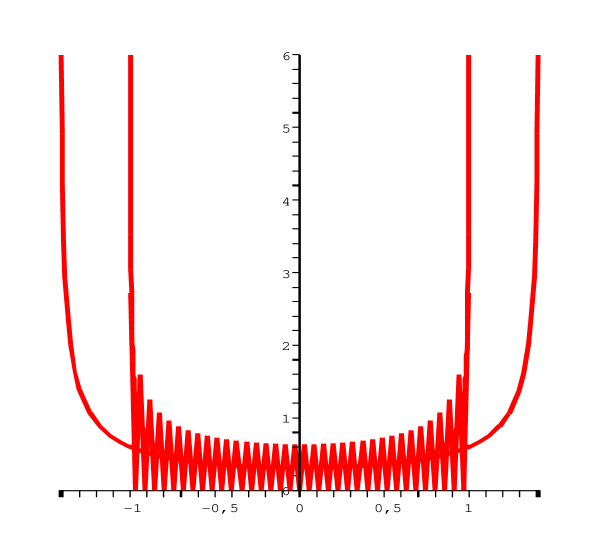
Figure 1: The double horn shaped limit probability distribution function for the QRW of the $V^{2}$ model is given in the plot. Also superimposed to it are given the occupation probabilities of the walk as evaluated after $n=36$ evolution steps. The more spread distribution in the graph is the distribution in [30] rescaled appropriately for comparison.

Proceeding to evaluate the asymptotic pdf of the walk we need to resort to the concept of the dual of completely positive trace preserving map[26]. Consider the dual map $\varepsilon_{V^{k}}^{\ast}$ $:B(H_{W})\rightarrow B(H_{W}),$ defined on the set of bounded operators acting on the walker Hilbert space $H_{W},$ of some given CPTP map $\ \varepsilon_{V^{k}}:D(H_{W})\rightarrow D(H_{W}),$ operating on the density matrices $\rho_{W}\in D(H_{W})$, with operator sum realization $\varepsilon_{V^{k}}(\rho_{W})=\sum_{i=\pm}A_{i}(k,\Phi;c)\rho_{W}A_{i}(k,\Phi;c)^{\dagger}.$ This dual map is defined to act on bounded operators $X\in B(H_{W}),$ as $\varepsilon_{V^{k}}^{\ast}(X)=\sum_{i=\pm}A_{i}(k,\Phi;c)^{\dagger}XA_{i}(k,\Phi;c)$ . By virtue of the last definition the expectation value (quantum moments) of the scaled powers of position operator $(\frac{L}{n})^{s},$ evaluated after $n$ steps of the walker which is now in the state $\rho_{W}^{(n)}=\varepsilon_{V^{k}}^{n}(\rho_{W}),$ become $\langle(\frac{L}{n})^{s})\rangle_{n}=Tr\left(\rho_{W}^{(n)}(\frac{L}{n})^{s}\right),$ or dually is determined by the equation $\langle(\frac{L}{n})^{s}\rangle_{n}\equiv\langle\varepsilon_{V^{k}}^{\ast n}((\frac{L}{n})^{s})\rangle_{0}\equiv Tr\left(\rho_{W}\text{ }\varepsilon_{V^{k}}^{\ast n}((\frac{L}{n})^{s})\right).$ Specializing to the $V^{2}$ model, and taking the case where initially $\rho_{W}=\left|0\right\rangle\left\langle 0\right|,$ and $\rho_{C}=\left|c\right\rangle\left\langle c\right|,$ with $\left|c\right\rangle=\cos\chi\left|+\right\rangle+i\sin\chi\left|-\right\rangle,$ we get the limit

$$\lim_{n\rightarrow\infty}\left\langle\varepsilon_{V^{2}}^{\ast n}\left((\frac{L}{n})^{s}\right)\right\rangle_{0}=\int_{0}^{2\pi}h(\phi)^{s}\frac{d\phi}{2\pi}=\int_{-1}^{1}\frac{y^{s}}{\pi\sqrt{1-y^{2}}}dy.$$ (8)

The resulting value of the quantum moment is seen in the last equation to be given as a statistical moment of the random variable $y^{s}$ with respect to the limit pdf determined as follows

$$P(y)=\frac{1}{\pi\sqrt{1-y^{2}}},\text{ }-1\leq y\leq 1.$$ (9)

This pdf, which is the same as that obtained in [29], determines asymptotically the occupation probabilities for the scaled position variable of our QRW. In figure (1) we present its graph which has the shape of a double horn peaked at the position $y=\pm 1.$ This is very much in difference with the Gaussian shape of the limit pdf that occurs in a classical random walk, but shares the double horn shape with the limit pdf of another model of QRW[7],[8], although the two distributions differ in their exact functional form. Also in the figure we have included the position occupation probabilities of the QRW after a large number of steps, in order to show their tendency towards their asymptotic values.

3 QRW Driven by Quantum Optical Cavity

We consider now an optical cavity where an interaction between a single electromagnetic (EM) mode and a single two-level atomic system takes place on resonance. Four different types of this interaction will be considered giving rise to four respective solvable models. These are the Jaynes-Cummings model (JCM) $H_{JCM},$ the intensity dependent JCM $H_{ID-JCM},$ the two photon JCM $H_{2ph-JCM},$ and the $m-$photon JCM $H_{mph-JCM},$ with the corresponding Hamiltonians given below:

$$H_{JCM} = \frac{\omega}{2}\sigma_{3}+\omega a^{\dagger}a+\lambda(\sigma^{+}a+\sigma^{-}a^{\dagger}),$$ (10)

$$H_{ID-JCM} = \frac{\omega}{2}\sigma_{3}+\omega a^{\dagger}a+\lambda(\sigma^{+}a\sqrt{N}+\sigma^{-}a^{\dagger}\sqrt{N+1}),$$ (11)

$$H_{2ph-JCM} = \frac{\omega}{2}\sigma_{3}+\omega a^{\dagger}a+\lambda(\sigma^{+}a^{2}+\sigma^{-}a^{\dagger 2}),\text{ and}$$ (12)

$$H_{mph-JCM} = \frac{\omega}{2}\sigma_{3}+\omega a^{\dagger}a+\lambda(\sigma^{+}a^{m}+\sigma^{-}a^{\dagger m}).$$ (13)

In the above expressions $a^{\dagger},$ $a$  are the creation, annihilation operators of quanta of the EM field satisfying the canonical commutation relation $[a,a^{\dagger}]=\mathbf{1}$, while the $\sigma^{+},\sigma^{-}$ realize the step operators in the atomic ”quantum coin” system state space, which together with $\sigma_{3}$ satisfy the Pauli matrix algebra $[\sigma_{+},\sigma_{-}]=2\sigma_{3},$ $[\sigma_{3},\sigma_{\pm}]=\pm\sigma_{\pm}$ . Also $\lambda$ is the field-atom coupling constant and $\omega$ stands for the atomic energy difference which equals the field frequency in the case of resonance, as in our case.

The dynamic symmetry of the above Hamiltonians can be seen by writing them as $\ H_{k}=C+V_{k},$ $k=$JCM,ID-ICM, $2$ph-JCM, mph-JCM, where $C=\frac{\omega}{2}\sigma_{3}+\omega N,$ with $N=a^{\dagger}a$ the number operator, is the common free part of the Hamiltonians and represents the total ”number of excitations” and the $V_{k}$ obviously identified with the rest part of the Hamiltonian stands for the interaction between atom and the field. We can verify the following constants of motion: $[H_{k},C]=0,$ $[H_{k},V_{k}]=0,$ $[C,V_{k}]=0.$

In the interaction picture the unitary evolution operator reads for each of these models $U_{k}(t)=\exp(-itV_{k}).$ Explicitly we obtain

$$U_{JCM}(t) = \left(\begin{array}[]{cc}\cos(\lambda t\sqrt{aa^{\dagger}})&-ia\frac{\sin(\lambda t\sqrt{a^{\dagger}a})}{\sqrt{a^{\dagger}a}}\\ -ia^{\dagger}\frac{\sin(\lambda t\sqrt{aa^{\dagger}})}{\sqrt{aa^{\dagger}}}&\cos(\lambda t\sqrt{a^{\dagger}a}\end{array}\right),\text{ \ }$$ (16)

$$U(t)_{ID-JCM} = \left(\begin{array}[]{cc}\cos(\lambda t\text{ }aa^{\dagger})&-ia\sqrt{N}\frac{\sin(\lambda t\text{ }a^{\dagger}a)}{a^{\dagger}a}\\ -i\sqrt{N}a^{\dagger}\frac{\sin(\lambda t\text{ }aa^{\dagger})}{aa^{\dagger}}&\cos(\lambda ta^{\dagger}a)\end{array}\right)$$ (19)

and for the $m-$photon case

$$U_{mph-JCM}(t)=\left(\begin{array}[]{cc}\cos(\lambda t\sqrt{a^{m}a^{\dagger m}})&-ia^{m}\frac{\sin(\lambda t\sqrt{a^{\dagger m}a^{m}})}{\sqrt{a^{\dagger m}a^{m}}}\\ -ia^{\dagger m}\frac{\sin(\lambda t\sqrt{a^{m}a^{\dagger m}})}{\sqrt{a^{m}a^{\dagger m}}}&\cos(\lambda t\sqrt{a^{\dagger m}a^{m}})\end{array}\right),$$ (20)

which is specialized to the case of two-photonic transition when $m=2.$ Assuming the initial field state is the pure state $\rho_{f}=|f\rangle\langle f|,$ and the atomic coin state the general density matrix $\rho_{C},$ the state of the atomic system after its crossing through the first quantum optical cavity is now described by the reduced density matrix given below which is obtain by tracing out the field degree of freedom namely,

$$\varepsilon_{U}(\rho_{C})=Tr_{f}\left(U(t)(\rho_{C}\bigotimes\rho_{f})U(t)^{\dagger}\right).$$ (21)

Introducing the operators $P_{ij}=|i\rangle\langle j|$ in the quantum coin space, then the map

$$\varepsilon_{U}(\rho_{C})=\sum_{ij,kl=0,1}P_{ij}\rho_{C}P_{kl}\langle f|U_{kl}^{\dagger}U_{ij}|f\rangle,$$ (22)

is a positive and trace preserving transformation of the atomic density matrix i.e if $\rho_{C}>0,$ then $\varepsilon_{U}(\rho_{C})>0,$ and also $Tr(\varepsilon_{U}(\rho_{C}))=Tr\rho_{C},$ as is easily shown. For the particular case of the JCM with the field been initially in the vacuum state i.e $|f\rangle=|0\rangle,$ we obtain the map

$$\varepsilon_{U}(\rho_{C})=S_{0}\rho_{C}S_{0}^{\dagger}+S_{1}\rho_{C}S_{1}^{\dagger}$$ (23)

where the so called Kraus generators of that map are

$$S_{0}(t)=\left(\begin{array}[]{cc}\cos(\lambda t)&0\\ 0&1\end{array}\right),\text{ }S_{1}(t)=\left(\begin{array}[]{cc}0&0\\ \sin(\lambda t)&0\end{array}\right),$$ (24)

and satisfy the property $S_{0}^{\dagger}S_{0}+S_{1}^{\dagger}S_{1}=\mathbf{1.}$

The generalization of this result to the case of all four models when the field is in some sharp number state $|f\rangle=|r\rangle$ $r=0,1,2,...,$ leads to the reduced coin density matrix

$$\varepsilon_{U}(\rho_{C})=A_{1}\rho_{C}A_{1}^{\dagger}+A_{2}\rho_{C}A_{2}^{\dagger}+A_{3}\rho_{C}A_{3}^{\dagger}$$ (25)

with Kraus generators

$$A_{1} = \left(\begin{array}[]{cc}\cos(\lambda t\eta)&0\\ 0&\cos(\lambda t\theta)\end{array}\right),\text{ }A_{2}=\left(\begin{array}[]{cc}0&0\\ \sin(\lambda t\eta)&0\end{array}\right),\text{ }$$ (30)

$$A_{3} = \left(\begin{array}[]{cc}0&\sin(\lambda t\theta)\\ 0&0\end{array}\right),$$ (33)

where $\eta=$ $\sqrt{r+1},r+1,\sqrt{(r+1)(r+2)},\sqrt{\frac{(r+m)!}{r!}}$ and $\theta=\sqrt{r},r,r(r-1),$ $\sqrt{\frac{r!}{(r-m)!}},$ are the angles for the respective models viz. the JCM, the ID-JCM, $2$-photon, and the $m$-photon JCM. The trace preservation of this map requires that $A_{1}^{\dagger}A_{1}+A_{2}^{\dagger}A_{2}+A_{3}^{\dagger}A_{3}=\mathbf{1}.$

4 Cavity Driven QRW Statistics

The effect of the first optical cavity will be to transform $\rho_{C}=\left|c\right\rangle\left\langle c\right|$ to $\varepsilon_{U}(\rho_{C}),$ this yields for the particular choice of $|c\rangle=\cos\chi|+\rangle+i\sin\chi|-\rangle,$ the mixed coin state

$$\varepsilon_{U}(\rho_{C}) = \frac{1}{2}\mathbf{1}+\frac{1}{2}\sin(2\chi)\cos\left(\ \lambda\eta t\right)\cos\left(\ \lambda\theta t\right)\sigma_{2}$$ (34)

$$+\frac{1}{2}\left[\cos\left(2\lambda\eta t\right)\cos^{2}\chi-\cos\left(2\lambda\theta t\right)\sin^{2}\chi\right]\sigma_{3}.$$

In this  case the characteristic function is time dependent and reads

$$h(\phi;t) = \left[-\cos\left(2\lambda t\eta\right)\cos^{2}\chi+\cos\left(2\lambda t\theta\right)\sin^{2}\chi\right]\cos(2\phi)$$ (35)

$$+\left[\sin(2\chi)\cos\left(\ \lambda t\eta\right)\cos\left(\ \lambda t\theta\right)\right]\sin(2\phi).$$

We now proceed to evaluate the limit probability distribution function, and to this end we rewrite the last equation as $h(\phi;t)=C(t)\cos[2\phi-\Lambda(t)]$, where we have introduce the functions $A(t)=-\cos\left(2\lambda t\eta\right)\cos^{2}\chi+\cos\left(2\lambda t\theta\right)\sin^{2}\chi,$ $B(t)=\sin(2\chi)\cos\left(\ \lambda t\eta\right)\cos\left(\ \lambda t\theta\right)$ from which we define the two functions $C(t)=\sqrt{A(t)^{2}+B(t)^{2}}$,  and $\tan\Lambda(t)=\frac{B(t)}{A(t)}$.  If we now set $y=h(\phi;t)$ then for all four inverses $h_{i}^{-1},$ $i=1,2,3,4,$ we get that $h^{\prime}(h_{i}^{-1}(y))=-2\sqrt{C(t)^{2}-y^{2}}$. This results into the limit pdf which is $P(y;t)=\frac{1}{2\pi}\sum\limits_{i}\frac{1}{|h^{\prime}(h_{i}^{-1}(y))|}$, or finally

$$P(y;t)=\frac{1}{\pi\sqrt{C(t)^{2}-y^{2}}},\text{ }-1\leq y\leq 1.$$ (36)

The influence of the first cavity is now expressed by the double dependence of the distribution, first on the time spent in the cavity i.e the coin-field interaction time, and second on the initial coin state by means of the dependence of $C(t),$ via $A(t)$ and $B(t),$ on the angle $\chi$ of the coin vector. The relationship

$$\int_{-1}^{1}\frac{dy}{\sqrt{1-y^{2}}}=\int_{-|C(t)|}^{|C(t)|}\frac{dy}{\sqrt{C(t)^{2}-y^{2}}}$$ (37)

between the limit distribution of the walk without the driving cavity (eq.(9)), and the same one with the driving cavity in presence (eq.(36)), shows that when $C(t)$ is not zero the asymptotics of QRW are robust to the changes caused by the modified coin system, up to a scaling. The scaling explicitly refers to the changes $y(t)\rightarrow y(t)/|C(t)|,$ $(-1,1)\rightarrow(-|C(t)|\rightarrow|C(t))|,$ in the random variable and its interval of values respectively.

Next, in figure (2), we give the graph of eq.(36) at various non zero values of $C(t).$

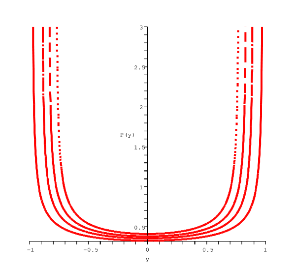
Figure 2: The limit pdf of fig.(1), as it has been affected by the presence of the optical cavity. The parameters $t$ and $\chi,$ are chosen so the function $C(t)^{2},$ modifying the limit pdf (see text), takes the values $C(t)^{2}=\{0.95,0.8,0.7,0.6\}.$ The respective plots are with solid line, dotted line, dashed line, and dashed-dotted line. Apart from scaling, the limit pdf reappears in the asymptotics of the walk. This scaling would lend itself to experimental detection of the robustness of the asymptotic pdf of the quantum walk.

The statistical moment derived by the new distribution are now in general time dependent, e.g the first two of them are found to be

$$\mu = \lim_{n\rightarrow\infty}\langle\frac{L}{n}\rangle_{n}=\int_{0}^{2\pi}h(2\phi;t)\frac{d\phi}{2\pi}=0,$$ (38)

$$\sigma(t)^{2} = \lim_{n\rightarrow\infty}\langle\left(\frac{L}{n}\right)^{2}\rangle_{n}\text{ }=\int_{0}^{2\pi}h(2\phi;t)h(\phi;t)^{2}\frac{d\phi}{2\pi}=\frac{C(t)^{2}}{2},$$ (39)

namely the first one is zero so that the walk remains unbiased while the standard deviation depends on the time spent by the coin in the first cavity.

To further probe the behavior of the QRW and especially the influences upon its asymptotics of the driving cavity, we first note that for $t=0,$ that is in the absence of the first cavity, the function $h$ depends on the initial state of the quantum coin system by means of its angle $\chi$ i.e $h(\phi;0)=-\cos(2\phi+2\chi).$ However this dependence does not show up in the asymptotic regime since its probability distribution given in eq.(9 ), appears to have a universal character, and is independent from the initial coin state provided it is of the form considered here.

On the other hand as eqs.(35,36) indicate in the case that there is a first cavity present the dependence of function $h$ on the initial coin state survives in the asymptotic regime for the $JCM$ and its variations. Indeed by inspection of the functions $A(t),$ $B(t)$ and $C(t)$ as given above we see that they do depend on the $\chi$ angle, and this dependence harbors the possibility of controlling the asymptotic statistics of the walk. By choosing the initial coin state to have angles $\chi=\{0,\frac{\pi}{2},\pi,\frac{3\pi}{2}\},$ namely to be $|c\rangle=\{|+\rangle,i|-\rangle,-|+\rangle,-i|-\rangle\}$ respectively, we enforce $B(t)=0,$ $\forall t.$ If we further choose the interaction time in the first cavity so that $A(t)=0,$ which implies correspondingly the times $t=\{\frac{(2k+1)\pi}{4\lambda\eta},$ $\frac{(2k+1)\pi}{4\lambda\theta},\frac{(2k+1)\pi}{4\lambda\eta},$ $\frac{(2k+1)\pi}{4\lambda\theta}\},$ $k\in Z$, then we get also $C(t)=0$ for those values of $t.$ Then the specific relations among the four coin states and interaction times as given above result into only two different pairs of coin density matrices and interaction times namely, $\rho_{C}=|+\rangle\langle+|,$ $t=\frac{(2k+1)\pi}{4\lambda\eta},$ and $\rho_{C}=|-\rangle\langle-|,$ $t=\frac{(2k+1)\pi}{4\lambda\theta},$ for which $C(t)=0,$ a fact that holds true for all JC models of our study. If each of these two conditions occur we say that a resonance condition takes place in the first cavity between the field and the two level atom.  So we see that the resonance condition implies that the standard deviation becomes zero, hence the limit pdf collapses, and more importantly that $<L^{2}>_{n}$ $\sim n,$ so we loose the quadratic diffusion time speed up, characterizing the quantum random walk. In such a case the asymptotic behavior of the standard deviation agrees with that of a classical random walk. More precisely what happens is that in all the above cases, the exiting coin from the first cavity is in the maximally classically mixed state $\rho_{C}=\frac{1}{2}|+\rangle\langle+|+\frac{1}{2}|-\rangle\langle-|$ $=\frac{1}{2}\mathbf{1}.$ If this coin system is used to feed in the second cavity where the $V^{2}$ QRW takes place, then the final one-step density matrix for the walker system becomes

$$\rho_{W}\rightarrow\varepsilon_{V^{2}}(\rho_{W})=\frac{1}{2}\rho_{W}+\frac{1}{4}E_{+}^{2}\rho_{W}E_{+}^{\dagger 2}+\frac{1}{4}E_{-}^{2}\rho_{W}E_{-}^{\dagger 2}.$$ (40)

A comment is on order. If $\rho_{W}$ is initially a diagonal matrix then so is finally, because of the last equation. Hence we really have a classical one-step transition that leads to Gaussian statistics for large $n,$ once we normalize $L$ to $\frac{L}{\sqrt{n}}$ . This implies that on resonance the walk becomes fully classical. This analysis makes obvious the fact that a judicious choice of the initial coin state permits us to tune the interaction time in the first cavity where the JCM or some of its variations is implemented, so that we have an absolute control not only over the asymptotic behavior of QRW, but on the very quantum nature of its performance as well. This conclusion makes the quantum optical experimental investigation of this idea worthwhile.

5 Conclusions

The QRW of the model $V^{2}$ exhibits a quadratically enhanced diffusion rate compared to the rate of the classical walk, and an interesting and counter intuitive  limit probability distribution. This distribution has been investigated in the present work with respect to its behavior under variations of the quantum coin state that are tailored in a cavity preceding the black box structure where the QRW itself is implemented. As the quantum coin is taken to be a two-level atom, its state alterations have been induced by letting it interact with a quantum mode in a JCM type of interaction on resonance. To gain generality in addition to the original JCM, three of its versions namely the intensity dependent, the two-photon and the $m-$ photon JCM have been used. All four models give rise to similar alteration of the asymptotics of the walk, a fact that shows the generality of the obtained results concerning asymptotics.

The two main modifications found of the long time limit probabilities of the QRW, are parametrized by the state of the coin going into the cavity, and the time spent by the coin in the cavity. In the first modification, the tuning of these two parameters to the resonance condition leads to fully classical results, namely to Gaussian limit distribution. In the second modification, a complementary situation prevails in which the double horn shape limit pdf re-emerges up to a scaling. These phenomena are independent of the particular version of the resonant JCM used to realize the driving cavity. Their experimental verification seems to be feasible by the present cavity QED experimental settings. Additional studies about e.g. the role of interaction time variations, the decoherence due to spontaneous emission of quantum coins, and the statistics of the arrival times of  quantum coins in the cavity, are necessary, and will be taken up elsewhere.

References

• [1] J. Kempe, Contemp. Phys. 44, 307 (2003).
• [2] M. A. Nielsen and I. L. Chuang, Quantum Computation and Quantum Information (CUP, Cambridge, 2000).
• [3] Y. Aharonov et al, Phys. Rev. A  48, 1687 (1992).
• [4] D. Meyer, J. Stat. Phys. 85, 551 (1996).
• [5] A. Ambainis et al, Proc. 33rd Annual Symp. Theory Computing (ACM Press, New York, 2001), p.37.
• [6] D. Aharonov et al, Proc. 33rd Annual Symp. Theory Computing (ACM Press, New York, 2001), p.50.
• [7] N. Konno, Quant. Inf. Proc. 1, 345 (2002).
• [8] G.Grimmett, S. Janson and P. F. Scudo, arXiv:quant-ph/0309135.
• [9] A. Nayak and A. Vishwanath, arXive eprint quant-ph/0010117.
• [10] C. Moore and A. Russell, Proc. RANDOM 2002, Eds. J.D.P Rolim and S. Vadhan, (Cambridge MA, Springer 2002), p. 164.
• [11] J. Kempe, Proc. RANDOM ;2003, Lect. Notes in Comp. Sci. 2764:354 , (2003).
• [12] A. Childs et. al, Quantum Information Processing 1, 35 (2002).
• [13] A. Childs et. al, arXive eprint quant-ph/0209131.
• [14] A. J. Bracken, D. Ellinas and I. Tsohantjis, J. Phys. A. Math. Gen. 37, L91 (2004).
• [15] B. C. Travaglione and G. J. Milburn, Phys. Rev. A 65, 032310 (2002).
• [16] W. Dur et al, Phys. Rev. A 66, 052319(2002).
• [17] B. C. Sanders et al, Phys. Rev. A 48, 1687 (1992).
• [18] D. Ellinas, On Algebraic and Quantum Random Walks, Quant. Prob. Inf. Dim.Analysis Vol. 18, Eds. M. Schörmann and U. Franz, (World Scientific 2005) p. 37.
• [19] D. Ellinas and I. Smyrnakis, to appear.
• [20] E. T. Jaynes and F. W. Cummings, Proc. IEEE 51, 89 (1963).
• [21] S. Stenholm, Phys. Rep. 6, 1 (1973).
• [22] J. H. Eberly, N. B. Narozhny and J. J. Sanchez-Modragon, Phys. Rev. Lett. 44, 1323 (1980); B. Narozhny, J. J. Sanchez-Modragon and J. H. Eberly, Phys. Rev. A. 23, 236 (1981).
• [23] B. Buck and C. V. Sukumar, Phys. Lett. 81A, 132 (1981).
• [24] C. V. Sukumar and B. Buck, ibid. 83A, 211 (1981).
• [25] S. Singh, Phys. Rev. A, 25, 3206 (1982).
• [26] K. Kraus, States, Effects and Operations (Springer-Verlag, Berlin, 1983).
• [27] B.G. Englert, M. Loffler, O. Benson, B. Varcoe, M. Weidinger and H. Walther, Fortschr. Phys. 46, 897 (1998).
• [28] J.M. Reimond, M. Brune and S. Haroche, Rev. Mod. Phys. 73, 565 (2001).
• [29] N. Konno, Continuous-Time Quantum Walk on the Line, quant-ph/0408140.
• [30] N. Konno, A New Type of Limit Theorems for the One-Dimensional Quantum Random Walk, quant-ph/0206103.