Quantum Computation by Communication

Abstract

We present a new approach to scalable quantum computing—a “qubus computer”—which realises qubit measurement and quantum gates through interacting qubits with a quantum communication bus mode. The qubits could be “static” matter qubits or “flying” optical qubits, but the scheme we focus on here is particularly suited to matter qubits. There is no requirement for direct interaction between the qubits. Universal two-qubit quantum gates may be effected by schemes which involve measurement of the bus mode, or by schemes where the bus disentangles automatically and no measurement is needed. In effect, the approach integrates together qubit degrees of freedom for computation with quantum continuous variables for communication and interaction.

I Introduction

Quantum computing has reached a very interesting stage in its development. Over the last decade there have been numerous proposals for qubit realisations fort00 . Some of the more mature proposals, such as trapped ions cirzol95 , nuclear spins (in molecules in liquid state) nmr97 and photonic qubits klm01 have now been demonstrated to work in the laboratory at the few-qubit level. Now in terms of their long term prospects for scalability, there is deemed to be considerable promise in “solid state” qubits, based (directly or indirectly) on fabrication and technologies developed for conventional IT. However, at present such approaches lag behind the more mature ones— they are either still on the drawing board, or at the one- or two-qubit demonstration level. The promise of scalability has yet to achieved for these approaches, and over the next few years it will be interesting to see which systems can meet this challenge and which founder.

Clearly decoherence and measurement are both important and challenging issues for solid state qubits. With the current emergence of demonstration qubit experiments, there is optimism about these problems being solved to a level that would permit useful small-scale quantum processing. However, even if these problems can be solved, there is still a need for two-qubit quantum gates to be implemented in a manner that enables the addition of more qubits to a system, so there is scalability. This is the main issue that we address in this paper. If these gates are implemented through a direct qubit-qubit interaction (i.e. a direct qubit-qubit coupling term in the basic system Hamiltonian), potential problems with two-qubit gates are: (i) the addition of an extra qubit to a system may disrupt the settings and calibrations that have been put in place for quantum computing with the original system, and (ii) the qubits may have to be so close together that individual addressing (both for single-qubit gates and measurement) cannot be achieved. Direct qubit interactions may be just fine for demonstrating entanglement between two solid state qubits, but they may not be as good when it comes to building a universal and scalable quantum processor. For example, with just nearest neighbour interactions there is a large SWAP operation overhead to interact chosen qubits, that could be removed through use of a bus to mediate interactions between non-nearest neighbours. One well known technique is to use single photons to mediate this interaction. There have been a number of very elegant proposals focusing on this, but they place highly stringent requirements, for example, on the generation of the single photons or their detection cir97 ; cir99 ; mancini04 ; duan04 ; lim05 ; duan05 ; barrett05 ; refwithin .

The approach that we present here contains no direct qubit-qubit interactions and does not require the use of single photons. Such interactions are achieved indirectly through the interaction of qubits with a common quantum field mode—a continuous quantum variable (CV) bra05 ; bra92 —which can be thought of as a communication bus lloyd00 . Our “qubus computer” approach brings together the best of both worlds. Static solid state qubits are used where they work best, for processing. Continuous variables are used where they work best, for communication and mediating interactions; they also have the potential to enable interfacing with existing, conventional information technology. We will assume that individual qubits can be prepared, subjected to single-qubit operations and measured. However, as we discuss in order to introduce our approach, interaction of a qubit with a CV bus mode, followed by measurement of the bus mode, can also be used in order to effect quantum non-demolition (QND) measurement of the qubit. This could be the preferred measurement scheme, unless something even better is achievable by other means. Our approach is based on qubits interacting with the bus mode through distinct dipole couplings, such as the electric dipole of a charge qubit coupling to the electric field quadrature, or the dipole of a spin or magnetic moment coupling to the magnetic field quadrature. The approach should be widely applicable in the solid state qubit context and so we present it in a generic fashion without being tied to any specific implementations.

As will be seen, our whole approach is based on the idea of a sequence of interactions, or gates, between qubits and the bus mode, followed by measurement of the bus in some scenarios, and not in others. The concept is therefore that qubits can be brought into interaction with the bus mode to effect the desired gate sequence, or that (certainly in the scenarios which involve bus measurement) a bus mode pulse can be employed to interact with successive qubits to effect the gate sequence. Our approach is thus to be contrasted with an “always on” interaction between qubits and a bus mode. In the latter case, such an interaction can in effect mimic a direct qubit-qubit coupling. For example, two qubits simultaneously coupled to a bus through the Jaynes-Cummings interaction behave as if they have a direct exchange interaction in the dispersive limit zhe00 ; ger05 . Instead, in our approach the qubit-bus interactions are sequential.

Following the generic formulation of our approach, we give an illustration applicable to superconducting charge qubits shn97 ; nak99 . The main results we present are methods for performing universal two-qubit gates mediated through a CV bus. Now in the superconducting scenario approaches have been proposed for using a common oscillator mode to effect qubit interactions mak99 ; bla04 , in effect by mimicking direct qubit-qubit interaction. It is also possible to consider an analogy with ion traps cirzol95 or cavity QED zheng04 for such solid state systems liu05 . Here we present a variety of schemes for two-qubit gates, which utilize a sequence of qubit interactions with the common bus mode in different ways, and which should be applicable to a wide range of matter qubit systems.

One approach we give requires no post-interaction work on the bus mode—it disentangles automatically from the qubits when the gate is done. Such schemes are analogous to ion trap gates which are insensitive to the vibrational state of the ions mil99 ; mol99 ; sor00 ; mil00 . This form of gate probably has the most widespread promise and long-term potential. However, it is also possible to effect gates that require a post-interaction measurement of the bus mode, based on recent ideas from non-linear quantum optics nem04 ; mun05b ; barrett05a ; mun05a ; barrett05b . These schemes may be preferable for some systems (certainly so if all the qubits couple to the same quadrature of the bus), and may also be the simplest approach for initial experimental investigations. They are also the natural extension of the QND measurement approach applied to two qubits, so we include discussion of various schemes of this form. In addition, the bus-measurement-free approach may be applicable in the field of non-linear quantum optics (or, more generally, where the interaction Hamiltonian has the characteristic cross-Kerr form), so we also include a discussion of this here.

We describe our qubits using the conventional Pauli operators, with the computational basis being given by the eigenstates of $\sigma_{z}$, with $|0\rangle\equiv|\uparrow_{z}\rangle$ and $|1\rangle\equiv|\downarrow_{z}\rangle$. The communication bus mode is described as a quantum field mode with creation(annihilation) operators $a^{\dagger}(a)$. For many solid-state qubits this could be an electromagnetic microwave field mode, although for other systems it may be an optical field. The centrepiece of our approach is an interaction Hamiltonian of the form

$$H_{int}=\hbar\chi\sigma_{z}X(\theta)$$ (1)

where $\sigma_{z}$ is the qubit operator and the field quadrature operator is $X(\theta)=(a^{\dagger}e^{i\theta}+ae^{-i\theta})$. Such an interaction Hamiltonian arises from the interaction between a charge qubit or Cooper pair box shn97 ; nak99 and the electromagnetic field, with the $z$ eigenstates representing the relevant two excess charge states of the box or island. Further examples include the interaction of a Cooper-pair box with a micromechanical resonator or cantilever arm02 , and other quantum electromechanical systems such as a Fullerene quantum dot which can both carry excess charge and vibrate mechanically wah04 . All of these systems can exhibit a very large electric dipole moment (compared to traditional atomic systems) and couple strongly to the relevant oscillator or field mode. The action of the Hamiltonian (1) for a time $t$ effects a displacement operation on the field of $D(\sigma_{z}\beta)$ inter-pic , conditioned on the state of the qubit, where $\beta=\chi te^{i(\theta-\frac{\pi}{2})}$ and $D$ is the usual displacement operator $D(\beta)=\exp(\beta a^{\dagger}-\beta^{*}a)$.

II Qubit measurement through controlled displacement

As an introduction to the use of a coherent bus mode we consider its application for measurement of a qubit. For the case of $\theta=\pi/2$ (coupling to the momentum quadrature in Eq. (1)), the displacements are in the $X(0)$ direction and, after interaction, an initial qubit-bus state of $|\Psi_{i}\rangle=(c_{0}|0\rangle+c_{1}|1\rangle)|\alpha\rangle$ is transformed to the entangled state

$$|\Psi_{f}\rangle=c_{0}|0\rangle|\alpha+\beta\rangle+c_{1}|1\rangle|\alpha-\beta\rangle\;.$$ (2)

The circuit diagram for this is shown in Fig. 1 for $\beta$ real. The effect of the interaction on the CV bus in phase space is illustrated in Fig. 2. Measurement of the bus mode can thus effect a non-demolition measurement of the qubit in its computational basis. The field measurement could be made by a homodyne measurement of the $X(0)$ quadrature, or an intensity measurement. This approach is the displacement-based analogue of photon non-demolition measurement based on an optical cross-Kerr non-linearity imo85 ; mil84 ; mun05 . Homodyne measurement of the bus mode, for example if this is a microwave field mode coupled to matter qubits, may be effected through a single electron transistor operated as a mixer saro05 , or some other suitable non-linear device, such as a superconducting Josephson ring system maria05 .

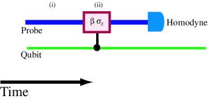
Figure 1: Circuit diagram for the QND measurement scheme based on conditional displacement of the bus mode by the qubit followed by a homodyne measurement on the bus mode.

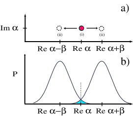
Figure 2: Schematic diagram showing the effect on the CV bus coherent state of interaction with the qubit (a). The coherent state is displaced conditional on the qubit state. The labels (i) and (ii) correspond to the evolution stages, as shown in the circuit diagram in the previous figure. (b) A schematic diagram of the $X(0)$ quadrature probability distribution for the CV bus mode state after interaction with the qubit. Clearly the qubit measurement is not perfect due to the overlap of peaks corresponding to different computational basis states.

Now clearly the qubit measurement is not perfect, as the final states of the CV bus mode corresponding to the different computational basis state amplitudes for the qubit are not exactly orthogonal, as illustrated in Fig. 2(b). However, for the example of taking the midpoint between the probability peaks as the discrimination point and using the $X(0)$ quadrature measurement of the bus, the error probability (the sum of the areas that sit the wrong side of the discrimination point) is $E=\frac{1}{2}$erfc$(2^{-1/2}|\beta|)$. This can be made very small for a suitable choice of $\beta$ mun05 , for example even for $|\beta|\sim 3$ the error is $E\sim 0.001$. Now this error formula and the example numbers are given on the basis of very accurate homodyne measurement of the CV mode quadrature. However, even somewhat imperfect homodyne measurement would still provide very good qubit measurement. The usual way to describe such an imperfect measurement is via a gaussian convolution of the ideal homodyne projectorWiseman93 ; Tyc04 , that is we use the projector $(2\pi\Delta)^{-1/2}\int_{-\infty}^{\infty}dy\exp[-(X-y)^{2}/(2\Delta)]|y\rangle\langle y|$ instead of $|X\rangle\langle X|$. The effect of this is to broaden the two distributions from a width of unity to a width of $1+\Delta$, which in turn means the overlap error function $E$ changes by a rescaling of $\beta$ to $\frac{\beta}{\sqrt{1+\Delta}}$. This can clearly still be kept small for a suitable choice of $\beta$.

This CV bus approach to solid state qubit measurement clearly has much promise. For example, it has already been realised wal05 for a superconducting charge qubit coupled to a microwave mode in the dispersive limit, when the qubit-cavity coupling effectively takes the form of a cross-Kerr non-linearity bla04 ; wal04 rather than that which generates controlled displacements.

III Two-qubit interaction through controlled bus displacement and measurement

Measurement of a coherent bus mode, following its interaction with two qubits, can be used to effect an entangling operation between the qubits. As an example, we again consider displacements in the $X(0)$ direction of the field. After the interactions, an initial two-qubit-bus product state of

$$|\Psi_{i}\rangle=\frac{1}{2}(|00\rangle+|01\rangle+|10\rangle+|11\rangle)|\alpha\rangle$$ (3)

is transformed to

$$|\Psi_{f}\rangle=\frac{1}{2}\left(|00\rangle|\alpha+2\beta\rangle+(|01\rangle+|10\rangle)|\alpha\rangle+|11\rangle|\alpha-2\beta\rangle\right),$$ (4)

assuming equal strength coupling of both qubits to the bus mode. Now if this procedure can be performed with the vacuum state ($\alpha=0$), then all is well and good. If not, an unconditional displacement operation $D(-\alpha)$ is applied to the bus mode prior to measurement. With this resolved, an appropiate measurement of the bus mode projects the two-qubit system into a maximally entangled state.

The corresponding circuit diagram for this operation is shown in Fig. 3. The evolution of the CV bus mode amplitudes is illustrated in Fig. 4. Now, for an ideal projection onto $|n\rangle$projection , the two-qubit state is conditioned to

$$|\psi_{f}\rangle=2^{-1/2}(|01\rangle+|10\rangle)$$ (5)

for $n=0$ and to

$$|\psi_{f}\rangle=2^{-1/2}(|00\rangle+(-1)^{n}|11\rangle)$$ (6)

for $n>0$. These projections happen with equal probability of $\frac{1}{2}$ (with the most likely value of $n$ in the latter case being $n\sim 4|\beta|^{2}$), although there is an error probability of $e^{-4|\beta|^{2}}$ (and a corresponding admixture to the state) in the former case, due to the overlap of the coherent state with the vacuum. This error can be made small for a suitable choice of $\beta$. The phase factor in the $n>0$ case is heralded by the measurement outcome $n$, and so can be allowed for or corrected.

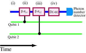
Figure 3: Circuit diagram for a two-qubit parity gate based on controlled displacements between the qubits and the “probe” bus, followed by bus measurement.

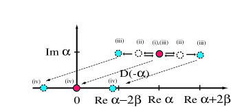
Figure 4: Schematic diagram showing the phase space evolution of the bus amplitudes corresponding to the various qubit computational basis states. The labels (i) to (iv) correspond to the evolution stages, as shown in the circuit diagram in Fig 3.

An alternative approach, which may be preferable in initial experiments, is to use an intensity measurement (or even a bucket detector), instead of a photon number resolving detector. In such a case the odd parity state is still projected to $|01\rangle+|10\rangle$, as in Eq. (5). However the even parity state of Eq. (6) $|00\rangle+(-1)^{n}|11\rangle$ becomes mixed, due to the uncertainty of whether $n$, although $>0$, is even or odd. The even parity state is thus represented by the density matrix $\rho=A\left[|00\rangle+|11\rangle\right]\left[\langle 00|+\langle 11|\right]+(1-A)\left[|00\rangle-|11\rangle\right]\left[\langle 00|-\langle 11|\right]$ where $A$ is determined by the distribution of the amplitudes $|00\rangle+|11\rangle$ and $|00\rangle-|11\rangle$ in the even parity subspace and any information obtained about $n$ from the measurement bucketdet . Now even in the worst case scenario ($A=1/2$) the protocol can be repeated, applying Hadamard operations ($|0\rangle\rightarrow|0\rangle+|1\rangle\;,\;|1\rangle\rightarrow|0\rangle-|1\rangle$) to the qubits and then interacting with the bus and measuring. Half the time, and heralded, this will give the odd parity pure state of Eq. (5) (which could be deterministically transformed to some other entangled state, as desired), and half the time a mixture will result. Thus after $m$ iterations the level of mixture will be $\sim(1/2)^{m}$, which can be made arbitrarily small by increasing $m$. Thus with multiples uses of a simple intensity measurement or bucket detector it is possible to generate a near-deterministic entangling operation between qubits, without the need for photon number resolution in the detection device applied to the bus clusterprep .

The entangling operation given in Eqs. (5) and (6), when operated with photon number resolution on the measurement, effectively projects the initial two-qubit state into an odd or even parity entangled state and, since the outcome is heralded by the measurement result, one could be transformed to the other, as desired. Whilst such a parity operation is not a unitary operation, it is possible to utilize this form of qubit parity operation along with single qubit rotations to construct a universal gate set nem05 . This has been shown in detail in the analogous case for optical qubits coupled to bus modes through cross-Kerr non-linearities nem04 ; mun05a . This analysis carries over in a straightforward manner to similar parity operations, however they are achieved. So, the displacement-based parity operation presented here provides a route to universal quantum processing for solid state qubits, all dipole-coupled to the same quadrature of a bus mode. It is also worth noting that under certain conditions the coupling of, for example, a charge qubit to a microwave field behaves like a cross-Kerr coupling, and so generates controlled rotations rather than controlled displacements on the field bla04 . In this limit the quantum optical approach to gates nem04 ; mun05b ; barrett05a ; mun05a carries over directly.

A further point to consider from the perspective of initial experiments is that it may be much easier to effect a probabilistic (but good fidelity) entangling operation, rather than the full parity gate. For example, homodyne measurement of the $X(0)$ quadrature of the CV bus mode applied directly to a system in the state of Eq. (4) will generate the two-qubit state of Eq. (5) probabilistically, but—very importantly—heralded by the quadrature result. As with the qubit measurement example, provided that $\beta$ is sufficiently large so the bus state probability distributions corresponding to the different two-qubit amplitudes in Eq. (4) have very little overlap, even a somewhat imperfect homodyne measurement of the bus quadrature can still give very high fidelity two-qubit entanglement. This probabilistic but heralded entangling operation is a good initial goal for experiments, prior to the full parity operation, leading further to a universal two-qubit gate.

IV Two-qubit gate through controlled bus displacements alone

Now there may be situations, such as initial experimental tests, or cases where in practice coupling to only one bus quadrature is possible, where it is desirable to effect a gate through qubit-bus interactions followed by a bus measurement. However, it is in fact possible to construct a universal two-qubit gate purely through a sequence of qubit-bus interactions, without the need for any subsequent measurement mil99 ; mil00 ; wan01 . This clearly simplifies the procedure, but it also has the potential for making the gate faster, as there is no need for measurement of the bus and qubit operations conditional on this result to complete the gate. One scheme to achieve such a gate requires one qubit (labelled 1) to be coupled to the momentum quadrature of the field ($\theta=\pi/2$ in Eq. (1)), thus generating displacements on the bus in the $X(0)$ direction, and the other qubit (labelled 2) to be coupled to the position quadrature ($\theta=0$ in Eq. (1)), giving displacements in the orthogonal direction.

With this arrangement and using the well-known result

$$D(\beta_{1})D(\beta_{2})=\exp\left[\frac{\beta_{1}\beta_{2}^{\ast}-\beta_{1}^{*}\beta_{2}}{2}\right]D(\beta_{1}+\beta_{2})\;,$$ (7)

the gate follows from four conditional displacements. The sequence of operations is shown in Fig. 5. This defines the unitary operator

$$U_{12}(\beta_{1},\beta_{2}) = D(i\beta_{2}\sigma_{z2})D(\beta_{1}\sigma_{z1})$$ (8)

$$\;\;\;\;\;\;\;\times D(-i\beta_{2}\sigma_{z2})D(-\beta_{1}\sigma_{z1})\;$$

For the case of real $\beta_{1}$ and $\beta_{2}$ the effect of this operator on the bus coherent state, conditional on the state of the qubits, is illustrated in Fig. 6. The action on the initial state of Eq. (3) is

$$|\Psi_{f}\rangle = U_{12}(\beta_{1},\beta_{2})|\Psi_{i}\rangle$$ (9)

$$= \frac{1}{2}\left(|00\rangle e^{2i\beta_{1}\beta_{2}}+|01\rangle e^{-2i\beta_{1}\beta_{2}}\right.$$

$$\;\;\;\left.+|10\rangle e^{-2i\beta_{1}\beta_{2}}+|11\rangle e^{2i\beta_{1}\beta_{2}}\right)|\alpha\rangle\;.$$

For any real value of $\beta_{1}\beta_{2}$ the bus mode is disentangled from the qubits at the end of the operation; nevertheless, for $2\beta_{1}\beta_{2}=\pi/4$ we obtain a maximally entangled state of the two qubits. In this case we achieve a universal two-qubit gate, which is equivalent to a controlled-phase gate (up to application of local unitaries $U_{i}=2^{-1/2}(1-i\sigma_{zi})$ to each qubit and a global phase of $\pi/4$). The bus mode enables the gate to be performed—it is certainly entangled with the qubits during the operation—but at the end of the gate it is disentangled and so has effectively played the role of a catalyst.

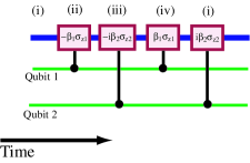
Figure 5: Circuit diagram of a universal two-qubit gate based on controlled displacements between the qubits and the ”probe” bus.

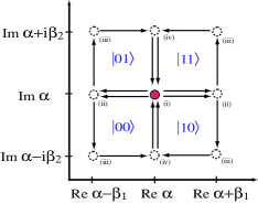
Figure 6: Schematic diagram showing the phase space evolution of the bus amplitudes for the four basis states of the two qubits. The labels (i) to (iv) correspond to the evolution stages, as shown in the circuit diagram in Fig. 5.

There are clearly numerous variations that can be made within this framework wan01 . The key features of the gate are:

1. It is the total phase space area traced out by a coherent state amplitude that determines the phase acquired by that amplitude wan01 . For a closed anticlockwise path $C$ in phase space

   $$\lim_{\Delta\alpha\rightarrow 0}\Theta\left(\prod_{i}D(\Delta\alpha_{i})\right)=\exp(2i\cal{A}_{C})\;,$$ (10)

   where $\Theta()$ reminds us that the operator order is preserved and the path $\{\Delta\alpha_{1},\Delta\alpha_{2},\dots\}$ forms a closed anticlockwise path $C$ in phase space. $\cal{A}_{C}$ is the area enclosed by $C$.

2. The fact that all the coherent state amplitudes end up on top of each other at the end of the gate disentangles the bus from the qubits without the need for any measurement of the bus mode.

There is a lot of freedom available within the constraints of achieving these features. For example, it may well be desirable to work with $\beta_{1}=\beta_{2}$ (so $\beta_{1}=(\pi/8)^{1/2}$ achieves the maximally entangling gate) or thereabouts, in order to minimise the total displacement for a given area. However, this is not necessary—different forms of qubit that couple to the bus mode with different strengths can be used, giving rectangular paths in phase space. Furthermore, the displacements do not have to be in orthogonal directions, although clearly a greater total displacement distance is required to achieve a given gate (such as a maximally entangling benchmark) if non-orthogonal displacements are employed. In general the shapes of the paths in phase space don’t matter; what is essential is that different two-qubit amplitudes effect different closed path areas on the bus, so that the phases acquired generate an entangling gate. In this sense the gate can be regarded as a geometric phase gate wan01 .

Although we have illustrated the gate with coupling to $\sigma_{z}$ for both qubits, other possibilities clearly also work. For example, if the coupling to qubit 1 is instead proportional to $X(\pi/2)\sigma_{x1}\equiv X(\pi/2)H_{1}\sigma_{z1}H_{1}$ (where $H_{1}$ is the Hadamard operation on qubit 1) then, subject to the same conditions as before (local unitaries $U_{i}=2^{-1/2}(1-i\sigma_{zi})$ applied to each qubit and a global phase of $\pi/4$), the two-qubit gate is equivalent to CNOT rather than a controlled-phase gate. This can easily be seen by starting with $|\Psi_{i}\rangle=2^{-1/2}(|00\rangle+|01\rangle)|\alpha\rangle$ rather than the state of Eq. (3). The approach therefore has significant flexibility in its ability to produce a universal two-qubit gate.

V Specific example—superconducting charge qubits

As a specific example we consider the case of superconducting charge qubits shn97 ; mak01 . Following the original demonstration of single charge qubit behaviour nak99 , there have been a number of experimental demonstrations of single vio02 ; yu02 ; mar02 and two-qubit pas03 ; yam03 ; ber03 ; mcd05 charge or charge-phase qubit behaviour, culminating in the recent demonstrations of coherent coupling to a bus mode wal05 ; wal04 . So such systems certainly form a promising route for our approach. A single charge qubit can be thought of as a very small superconducting island—a capacitor (of capacitance $C$)—with Josephson tunnel coupling (of Cooper pair charges $2e$) to a larger superconducting reservoir. The characteristic electrostatic energy of the system is $E_{c}=(2e)^{2}/2$ and the Josephson tunnelling energy is $E_{J}$. For qubit operation the system is biased with an external quasi-static voltage source ($V_{x}$) such that the states of the island with zero and one excess Cooper pair charge are near degenerate, and form a good approximation to a qubit computational basis. The size of the Josephson coupling $E_{J}$ can be varied externally by creating a composite junction from two parallel junctions in a loop threaded by a magnetic flux $\Phi_{xc}$.

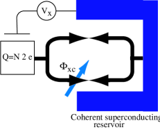
Figure 7: Schematic diagram of a charge qubit. A superconducting island with excess charge $2Ne$ is connected to a reservoir through a composite Josephson junction, whose effective tunnelling amplitude is controlled by the magnetic flux $\Phi_{xc}$. An external voltage bias $V_{x}$ is applied to induce an additional polarization charge.

Such a charge qubit is illustrated in Fig. 7. Putting these external sources in characteristic dimensionless terms ($n_{x}=CV_{x}/2e$, where $C$ is the effective capacitiance, and $\phi_{x}=2\pi\Phi_{xc}/\Phi_{0}$) the charge qubit Hamiltonian can be written as shn97 ; mak01 ; spil00

$$H_{cq}=E_{c}\sigma_{z}(n_{x}-\frac{1}{2})-E_{J}\sigma_{x}\cos\phi_{x}\;.$$ (11)

Now, viewed as a planar structure, if such a qubit is placed in a microwave field mode at a position where there is a non-zero electric field (denoted as the quadrature $X(0)$) across the capacitor and junction, there will be a microwave contribution to $n_{x}$ and thus a coupling of the desired form $X(0)\sigma_{z}$ wal05 ; bla04 . Consider two such charge qubits, with no direct coupling to each other but both positioned so they couple to the electric field antinode of a microwave mode. This is illustrated schematically in Fig. 8. The entangling gate based on controlled displacements followed by microwave field measurement described earlier could be applied to this two-charge-qubit system, either in its full form, or in its probabilistic heralded form. Given typical practical microwave wavelengths (cm maybe down to mm), clearly many micron-scale qubits could all be placed at the same bus field antinode, forming a useful quantum processor or register.

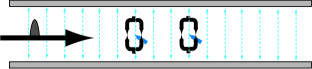
Figure 8: Schematic diagram of a two-charge-qubit system, with each qubit coupled to the electric field of a microwave bus mode.

Alternatively, if a charge qubit is at a position where there is a non-zero magnetic field (denoted as the quadrature $X(\pi/2)$) normal to the plane of the structure and threading the composite junction, there will be a microwave contribution to $\phi_{x}$ and coupling of the form $X(\pi/2)\sigma_{x}\sin\phi_{xqs}$, which is controllable through the quasi-static part of the field $\phi_{xqs}$. Consider two charge qubits, one positioned to couple to the electric field antinode of a microwave mode and the other positioned to couple to the magnetic field antinode of the same mode, as illustrated schematically in Fig. 9. With such a system it is clearly possible to realise couplings to different field quadratures, and thus perform a universal two-qubit quantum gate without any post-interaction measurement of the bus mode. As this form of gate links qubits at different field antinodes, this provides for distributed gates between qubits separated by cm/mm distances.

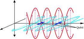
Figure 9: Schematic diagram of an array of planar charge qubits coupled to a common microwave bus mode. Adjacent qubits are respectively coupled to the antinode of the electric field (across the junction) and the antinode of the magnetic field (threading the composite junction loop), enabling the forms of coupling needed for the measurement-free gate.

There are clearly many other possibilities that can be considered. In terms of bus-measurement-enabled gates or interactions, different forms of charge qubit (e.g. superconducting and semiconducting) could be used. Gates between magnetic flux qubits Boc97 ; Moo99 ; chi03 , all coupled to the same magnetic field antinode of a microwave mode, could be effected through this approach. Experimental evidence for coherent coupling between a flux qubit and an electromagnetic oscillator has already been seen chi04 . Gates between flux qubits and other forms of magnetic qubit is a further possibility. In terms of measurement-free gates, it is possible to design a new form of charge qubit (including a $\pi$-junction) that enables geometric two-qubit gates through interaction with a common microwave bus zhu05 . Two-qubit interactions between charge and flux qubits (suitably positioned to couple to the relevant microwave field quadratures) is yet another possibility. A long term goal could therefore be a quantum computer architecture consisting of a sizeable register (of like qubits) suitably positioned at each microwave bus mode antinode, functioning through ”local” gates between qubits in the same register and distributed gates between qubits in different registers. Scaling up even further, it would be natural to consider multiple buses, each containing a multi-register processor, all coupled together to form a larger computer. However, at present clearly the most immediate goal is the experimental demonstration of local and distributed gates between an appropriate pair of qubits, mediated through a single microwave bus.

VI Two-qubit gate through controlled bus rotation and measurement

For some solid state qubit systems, or in certain limits of behaviour of some systems, the interaction with a bus mode takes the effective form of a cross-Kerr non-linearity (for instance see Ref bla04 ), analogous to that for optical systems (see appendix 1 for details). In this case we have an interaction Hamiltonian of the form

$$H_{int}=\hbar\chi\sigma_{z}a^{\dagger}a$$ (12)

rather than that of Eq. (1). When acting for a time $t$ on a qubit-bus system, this interaction effects a rotation (in phase space) of $\pm\theta$ on a bus coherent state, where $\theta=\chi t$ and the sign depends on the qubit computational basis amplitude. Now it is known already in the quantum optics context that such interactions can be used to effect a universal two-qubit gate between photonic qubits, based on bus measurement nem04 . Here we give two examples of a two-qubit parity gate, based on different forms of bus measurement.

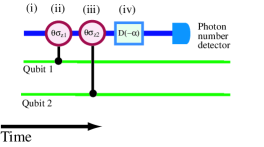
Figure 10: The circuit diagram for a two-qubit parity gate based on controlled rotations between the qubits and the probe bus, followed by bus number measurement.

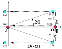
Figure 11: Schematic diagram showing the phase space evolution of the bus amplitudes corresponding to the various qubit computational basis states. The labels (i) to (iv) correspond to the evolution stages, as shown in the circuit diagram in the previous figure.

The circuit diagram for the first gate is shown in Fig. 10. Following the interactions and an unconditional displacement operation $D(-\alpha)$, an initial two-qubit-bus product state of Eq. (3) is transformed to

$$|\Psi_{f}\rangle=\frac{1}{2}\left(|00\rangle|\alpha(e^{2i\theta}-1)\rangle+(|01\rangle+|10\rangle)|0\rangle\right.$$

$$\left.+|11\rangle|\alpha(e^{-2i\theta}-1)\rangle\right),$$ (13)

assuming equal strength coupling of both qubits to the bus mode. This is illustrated schematically in Fig. 11. A photon number measurement applied to the bus mode clearly either picks out the vacuum, or projects onto the other two amplitudes without distinguishing them. Now, for $2\theta\ll 1$ and an ideal projection onto $|n\rangle$, the two-qubit state is conditioned to

$$|\psi_{f}\rangle=2^{-1/2}(|01\rangle+|10\rangle)$$ (14)

for $n=0$ and to

$$|\psi_{f}\rangle=2^{-1/2}(i^{n}|00\rangle+(-i)^{n}|11\rangle)$$ (15)

for $n>0$. These happen with equal probability of $\frac{1}{2}$ (with the most likely value of $n$ in the latter case being $n\sim 4|\alpha\theta|^{2}$), although there is an error probability of $e^{-4|\alpha\theta|^{2}}$ (and a corresponding admixture to the state) in the former case, due to the overlap of the coherent state with the vacuum. This error can be made small with a suitable choice of $\alpha$ for some given $\theta$. The phase factor in the $n>0$ case is heralded by the measurement outcome $n$, and so can be allowed or corrected for. Clearly using a photon number measurement this gate is near-deterministic. Alternatively one can also use the iterative procedure with the intensity measurement/bucket detector described in Section (III) to enable near-deterministic entanglement generation. If one is instead prepared to accept a probabilistic gate, heralded by the measurement outcome, then a measurement of the $X(\pi/2)$ quadrature of the bus can be used. Half the time it will project to Eq. (14), heralded by a result close to zero. The other half of the time no entanglement will be produced. Such a procedure may be a good approach for initial experimental demonstrations of the principle. It would not require the final unconditional displacement.

A near-deterministic gate based on a single final quadrature measurement can be achieved, although it requires a more involved circuit. This is shown in Fig. 12. Following qubit-bus interactions analogous to the previous gate and an unconditional displacement operation $D(-2\alpha\cos 2\theta)$, further qubit-bus interactions occur. An initial two-qubit-bus product state of Eq. (3) is transformed to

$$|\Psi_{f}\rangle = \frac{1}{2}\left[(|00\rangle+|11\rangle)|-\alpha\rangle\right.$$ (16)

$$\;\;\;\;+\left.(|01\rangle+|10\rangle)|\alpha(1-2\cos 2\theta)\rangle\right],$$

again assuming equal strength coupling of both qubits to the bus mode. This is illustrated schematically in Fig. 13. Clearly with this scheme a homodyne measurement of the $X(0)$ quadrature of the bus mode will project onto the odd or even parity entangled two-qubit states that sit in Eq. (16), with the outcome heralded by the quadrature result. This parity gate isn’t perfect, as the final states of the CV bus mode corresponding to the different entangled states of qubits are not exactly orthogonal. (See Fig. 2 for an illustration.) However, as with the qubit measurement scenario, for the example of taking the midpoint between the probability peaks as the discrimination point and using $X(0)$ quadrature measurement of the bus, the error probability (the sum of the areas that sit the wrong side of the discrimination point) is approximately $E=\frac{1}{2}$erfc$(2^{1/2}|\alpha|\theta^{2})$. This can be made very small for a suitable choice of $\alpha\theta^{2}$. As in the qubit measurement case, somewhat imperfect homodyne measurement can be tolerated provided that $\alpha\theta^{2}$ is large enough to dominate the homodyne error.

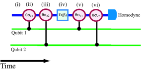
Figure 12: The circuit diagram for a two-qubit parity gate based on controlled rotations between the qubits and the probe bus, followed by bus $X(0)$ quadrature measurement. The amplitude of the unconditional displacement is given by $\beta=-2\alpha\cos 2\theta$.

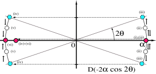
Figure 13: Schematic diagram showing the phase space evolution of the bus amplitudes corresponding to the various qubit computational basis states. The labels (i) to (vi) correspond to the evolution stages, as shown in the circuit diagram in the previous figure.

VII Two-qubit gate through controlled bus rotations alone

With cross-Kerr interactions of the form of Eq. (12) it is also possible to achieve a universal two-qubit gate without any bus measurement. The relevant gate sequence is illustrated in Fig. 14.

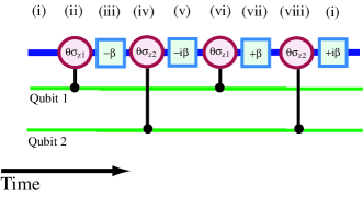
Figure 14: The circuit diagram of a two-qubit controlled-phase gate, based on controlled rotations between the qubits and the probe bus and non-controlled displacements of the bus.

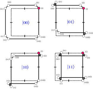
Figure 15: Schematic diagram showing the phase space evolution of the bus amplitudes corresponding to the various qubit computational basis states. The labels (i) to (viii) correspond to the evolution stages, as shown in the circuit diagram in the previous figure. The small areas shown in grey are traversed in a clockwise sense, giving a negative contribution to the phase acquired.

In this case the unconditional displacements are all of equal magnitude $\beta$ (but varying directions as shown in Fig. 14) and the controlled rotations are generated through Hamiltonians of the form (12) with an interaction time $t$ and $\theta=\chi t$. With an initial state of (3) and $\alpha=\beta(1+i)/2$, the gate sequence of Fig. 14 achieves a gate which is locally equivalent to a controlled-phase gate for the condition $|\beta\theta|^{2}=\pi/4$. The behaviour of the bus amplitudes in phase space is illustrated in Fig. 15. There are a number of points that should be noted about this gate.

1. There are simpler circuits available for the two-qubit gate through controlled bus rotations alone. These use the same number of controlled rotations but fewer probe bus displacement operations. For example, in the circuit given in Fig. 14, the final displacement is not actually necessary to implement the gate. In this case the final displacement just returns the probe beam to its initial starting position, which is neat but unnecessary.

2. There are also variations of these gates based on two displacement operations. Unfortunately, while performing a CNOT or CPhase, these do not have the same scaling in terms of $\theta$ and $\beta$ for the resultant phase shift.

3. In the rotation-based case of Fig. 15, unlike that of the displacement-based gate of Fig. 6, there is an error. The bus mode doesn’t disentangle from the qubits exactly, because the (small) rotations employed are arcs of circles, rather than straight lines. The error is of order $|\beta\theta^{2}|$, which can clearly be made small (of order $1/\beta$) even for a maximally entangling universal gate by working in the small $\theta$ large $\beta$ limit. The gate is discussed in more detail in the Appendix 2.

VIII Specific examples

It is already known theoretically bla04 that a superconducting charge qubit (as illustrated in Fig. 7) coupled to a microwave field mode in the dispersive limit has an interaction Hamiltonian of the cross-Kerr form of Eq. (12). Furthermore, experiments in this limit wal04 ; wal05 have clearly demonstrated this coupling. Such systems are clearly excellent candidates for the controlled-rotation-based gates that we propose. Two charge qubits coupled to a microwave field mode (as illustrated in Fig. 8) in the dispersive limit form a candidate system for realising the measurement-based gates. The simplest initial demonstration would probably be to employ the scheme given in Fig. 10 in a probabilistic approach, in which case the final non-controlled displacement is unnecessary. Measurement of the $X(\pi/2)$ quadrature of the microwave field would entangle the charge qubits with probability 1/2, heralded by a measurement outcome close to zero. If such a gate could be achieved, this would point the way towards the near deterministic gates of Figs. 10 and 12, based respectively on photon number or $X(0)$ quadrature measurement of the microwave field. With sufficient control over the couplings and the microwave field, the geometric gate of Fig. 14 between two dispersive charge qubits is a further possibility.

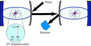
Figure 16: Schematic diagram of a two NV-diamond centre qubits in separate cavities coupled via a cross-kerr interaction to an optical field. The final measurement enables the construction of a parity gate. .

We can also consider NV-diamond centres martin99 ; jelezko04 within individual cavities as excellent matter system candidates for the qubus protocol and especially the parity gates (as depicted in Fig  16). Within the level structure of an NV-diamond centre are two long-lived states $|{\uparrow}\rangle$ and $|{\downarrow}\rangle$ and an excited state $|e\rangle$, in an $L$-configuration with the $|{\downarrow}\rangle\leftrightarrow|e\rangle$ transition coupled to the cavity mode. The $|{\uparrow}\rangle$ state can represent the logical $|0\rangle$ basis state and the $|{\downarrow}\rangle$ state the logical $|1\rangle$ basis state. The NV diamond level configuration is such that only the $|1\rangle$ state can be excited to the state $|e\rangle$ via an optical pulse while the $|0\rangle$ to $|e\rangle$ transition is assumed forbidden or extremely weak. When the optical pulse interacts with the $|1\rangle$ state, it picks up a small phase shift due to the $|1\rangle\leftrightarrow|e\rangle$ transition while no phase shift occurs for the $|0\rangle$ state. This essential difference is all that we require to create a conditional phase shift and thus implement the two qubit gates through controlled rotation.

IX Controlled displacements from controlled rotations

The previous sections have demonstrated the power of qubit-controlled displacements and rotations, applied to a communication bus, for fundamental two-qubit gate operations and quantum information processing. The controlled displacement gates seem potentially easier to implement, as they do not require unconditional displacements as well and operate for small to large values of $\chi t$. However the controlled displacement schemes generally have a strong dipole coupling requirement, needed to ensure that $\omega t$ can be assumed constant through out the gate. For SQUID and other microwave based schemes this condition can be satisfied easily, but it poses a significant problem in the optical regime, suggesting that optical schemes are restricted to controlled rotation based gates. However, this is not the case, as it is straightforward to transform a controlled rotation interaction to a controlled displacement. Consider the Hamiltonian in the interaction picture given by Eq. (12) with the bus mode displaced by an amount $\alpha$. In this case

$$\hbar\chi\sigma_{z}a^{\dagger}a\rightarrow\hbar\chi\sigma_{z}\left[|\alpha|^{2}+\alpha^{\ast}a^{\dagger}+\alpha a+a^{\dagger}a\right]\;.$$ (17)

If we let $\alpha=|\alpha|e^{-i\theta}$ then the above equation can be written in the form $H_{int}=\hbar\chi\sigma_{z}\left[|\alpha|^{2}+|\alpha|X(\theta)+a^{\dagger}a\right]$. We clearly see a controlled displacement term, plus two other pieces dependent on $a^{\dagger}a$ and $|\alpha|^{2}$. These terms can be eliminated with a simple trick as follows. First run the interaction given by $U(\alpha,\sigma_{z},t)=\exp\left[iH_{int}t/\hbar\right]$ for a time $t/4$, then bit-flip the qubit and change the sign of the displacement from $+\alpha\rightarrow-\alpha$ and run for a further time $t/2$. Finally repeat the orginal $U(\alpha,\sigma_{z},t)$ for a time $t/4$. This results in a net interaction $U(\alpha,\sigma_{z},t/4)U(-\alpha,-\sigma_{z},t/2)U(\alpha,\sigma_{z},t/4)\sim\exp\left[i|\alpha|\chi t\sigma_{z}X(\theta^{\prime})+O[t^{3},a,a^{\dagger}]\right]$ which is the desired displacement. There is now an effective coupling constant $|\alpha|\chi$, where $\alpha$ can in principle be large. There is a small $O(t^{3})$ correction in the above evolution but this is tiny for reasonable interaction times. The key issue becomes how to achieve the displacement on the probe field. There are a number of well known solutions to this but the easiest is to drive the probe field with a classical pump where the displacement is required. This is experimentally achievable.

It is worthwhile considering a specific situation in a litte more detail. Consider a Lambda-type atomic configuration with the two lowest energy levels representing the logical qubit states. We know that if we detune by $\Delta$ a field $a$ that connects the logical $|1\rangle$ to the excited state $|e\rangle$ we get an effective coupling $H_{I}=\hbar\frac{g^{2}}{2\Delta}a^{\dagger}a|1\rangle\langle 1|$, where $g$ is the coupling coefficient between the atomic system and probe mode. A second field $b$ detuned above the $|e\rangle$ by the same amount gives $H_{I}=-\hbar\frac{g^{2}}{2\Delta}b^{\dagger}b|1\rangle\langle 1|$. Now if we choose the field $a$ to have a large classical component, then $a\rightarrow a+|\alpha|e^{-i\theta}$ and the field $b$ to be pure classical $b\rightarrow|\alpha|e^{-i\phi}$ then the two effective Hamiltonian yields a net Hamiltonian

$$H_{eff}=\hbar\frac{g^{2}}{2\Delta}\left[|\alpha|X(\theta)+a^{\dagger}a\right]|1\rangle\langle 1|$$ (18)

where the quadratic Stark shift of the level $|1\rangle$ is cancelled and there is no special phase relation required between the upper and lower detunings. Lastly for $|\alpha|$ large the component $a^{\dagger}a|1\rangle\langle 1|$ can be neglected or eliminated as discussed above. There are many variations of this approach—the one to be used in practice depends upon the actual experimental system.

X A further example based on rotations and displacements

Finally, we present a near-deterministic gate based on a final quadrature measurement and with qubits that are able to both rotate and displace the bus mode. This may be rather more difficult to achieve for the current most popular matter qubits, in comparison to the gates already presented, but we include it to cover the full spectrum of possibilities. The circuit diagram is shown in Fig. 17.

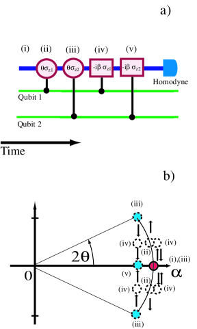
Figure 17: a) The circuit diagram of a two-qubit parity gate, based on controlled rotations and controlled displacements between the qubits and the probe bus. b) Schematic diagram showing the phase space evolution of the bus amplitudes corresponding to the various qubit computational basis states. The labels (i) to (v) correspond to the evolution stages, as shown in the circuit diagram in a).

Following this conditional gate sequence, an initial two-qubit-bus product state of Eq. (3) is transformed to

$$|\Psi_{f}\rangle=\frac{1}{2}\left((|00\rangle+|11\rangle)|\alpha(1-\cos 2\theta)\rangle\right.$$

$$\left.+(|01\rangle+|10\rangle)|\alpha\rangle\right),$$ (19)

assuming equal strength coupling of both qubits to the bus mode and $\beta=\frac{\alpha}{2}\sin 2\theta$. The phase space evolution of the bus mode amplitudes is illustrated schematically in Fig. 13. The result is two amplitudes lying on the real axis, so a homodyne measurement of the $X(0)$ quadrature of the bus mode will project onto the odd or even parity entangled two-qubit states that sit in Eq. (X), with the outcome heralded by the quadrature result. As with some previous examples, this parity gate isn’t perfect, as the final states of the CV bus mode corresponding to the different entangled states of qubits are not exactly orthogonal, as illustrated in Fig. 2. Once again, taking the midpoint between the probability peaks as the discrimination point, the error probability (the sum of the areas that sit the wrong side of the discrimination point) is approximately $E=\frac{1}{2}$erfc$(2^{-1/2}|\alpha|\theta^{2})$. This can be made very small for a suitable choice of $\alpha\theta^{2}$ and somewhat imperfect homodyne measurement can be tolerated provided that $\alpha\theta^{2}$ is large enough to dominate the homodyne error.

XI Discussion

We have presented a new approach to quantum computing—a “qubus computer”—which brings together discrete qubits with quantum continuous variables in a single scheme. Through interaction with a common bus mode, it is possible to realise a universal two-qubit gate. We considered three different schemes including:

• Measurement-based probabilistic but heralded parity gates,

• Measurement-based near deterministic parity gates and

• Measurement-free deterministic CPhase gates,

with two different interactions (the controlled-displacement and the controlled-rotation) between the discrete qubits and the bus mode. For the latter scheme, no post-interaction measurement is required on the bus mode — it effectively plays the role of a catalyst in enabling the gate. All of these approaches are particularly well suited for solid state qubits, which generally have a natural dipole coupling to a common electromagnetic field mode, such as superconducting qubits coupled to a microwave field or an NV diamond centre coupled to an optical cavity mode. However the results are also directly applicable to all optical gates.

Lastly, our approach does not generally force a choice of computation scheme and processor architecture; rather it provides building blocks which can be put together to suit the task at hand. For instance, the near deterministic gates can be used for the standard gate-based quantum computation as well computation by measurement (the one-way quantum computer Briegel01 ; Nielsen04 ; Browne04 for instance) or the simulation of Hamiltonians. Our approach requires only a practical set of resources, and it uses these very efficiently. Thus it promises to be extremely useful for the first quantum technologies, based on scarce resources. Furthermore, in the longer term this approach provides both options and scalability for efficient many-qubit quantum computation.

Acknowledgments: We thank R. Van Meter, S. D. Barrett, R. G. Beausoleil, P. Kok, T. Ladd and P. L. Knight for valuable discussions. This work was supported in part by the Japanese JSPS, MPHPT, and Asahi-Glass research grants, the UK research council EPSRC, the Australian Research Council Centre of Excellence in Quantum Computer Technology and the European Project RAMBOQ. SLB currently holds a Royal Society Wolfson Research Merit Award.

XII Appendix 1

Consider the three level Raman coupling scheme in a Lambda configuration. A strong coherent field is detuned from the dipole allowed transition $|0\rangle\leftrightarrow|e\rangle$, while a weaker cavity field (annihilation operator $a$) is detuned by an equal amount from the dipole transition $|1\rangle\leftrightarrow|e\rangle$. The effective two level Hamiltonian describing this Raman process isLeibfried

$$H=\hbar\frac{\omega_{0}}{2}\sigma_{z}+\hbar\omega_{c}a^{\dagger}a+\frac{\hbar\Omega}{2}(a\sigma_{+}+a^{\dagger}\sigma_{-})$$ (20)

where $\sigma_{z}=|0\rangle\langle 0|-|1\rangle\langle 1|,\ \ \ \sigma_{+}=|1\rangle\langle 0|$ and $\hbar\omega_{0}$ is the energy difference between the qubit states while $\omega_{c}$ is the frequency of the quantised cavity mode that acts as the quantum bus.

We now transform to an interaction picture by the unitary operator

$$U_{o}(t)=\exp[-i\frac{\omega_{0}}{2}\sigma_{z}t-i\omega_{c}a^{\dagger}at]$$ (21)

so that the state in the interaction picture satisfies

$$\frac{d|\psi(t)\rangle_{I}}{dt}=-\frac{i}{\hbar}H_{I}(t)|\psi(t)\rangle_{I}$$ (22)

where

$$H_{I}(t)=\frac{\hbar\Omega}{2}(a\sigma_{+}e^{-i\Delta t}+a^{\dagger}\sigma_{+}e^{i\Delta t})$$ (23)

and $\Delta=\omega_{c}-\omega_{0}$. The solution is

$$|\psi(t)\rangle_{I} = \left[1-\frac{i}{\hbar}\int_{0}^{t}dt_{1}H_{I}(t_{1})\right.$$

$$\left.+\frac{1}{2}(\frac{-i}{\hbar})^{2}\int_{0}^{t}dt_{2}\int_{0}^{t_{2}}dt_{1}H_{I}(t_{2})H_{I}(t_{1})+\ldots\right]$$

For sufficiently large detuning, the relevant time scale of the dynamics is such that $\Delta t>>1$. We can make the following approximations

$$\int_{0}^{t}dt_{1}H_{I}(t_{1}) \approx 0$$

$$\int_{0}^{t}dt_{2}\int_{0}^{t_{2}}dt_{1}H_{I}(t_{2})H_{I}(t_{1}) \approx -i\frac{\hbar^{2}\Omega^{2}}{4\Delta}(aa^{\dagger}\sigma_{+}\sigma_{-}-a^{\dagger}a\sigma_{-}\sigma_{+})$$

Continuing in this way we can find that all terms of odd order in $\Omega$ can be neglected, while all terms of order $\Omega^{2n}$ are proportional to $t^{2n}$, so that the dynamics can be approximated by

$$|\psi(t)\rangle_{I}=e^{-iH_{eff}t/\hbar}$$ (25)

where, by using the commutation relations, the effective interaction Hamiltonian can be written as

$$H_{eff}=\hbar\chi a^{\dagger}a\sigma_{z}$$ (26)

There is also a small renormalisation of the atomic and cavity frequencies that we have ignored.

XIII Appendix 2

It is worthwhile examining the two-qubit gate through controlled bus rotations alone in a little more detail, as there are a number of subtle issues in its operation. We will assume that the probe bus starts initially in the state $|\alpha e^{i\frac{\pi}{4}}\rangle$ with $\alpha$ real. The displacement is given $\beta=\sqrt{2}\alpha$. It is straighforward but tedious then to show that the four basis states (including the probe bus) evolve as

$$|g\rangle|g\rangle|\alpha e^{i\frac{\pi}{4}}\rangle \rightarrow e^{i\phi_{gg}}|g\rangle|g\rangle|\alpha_{+}\rangle$$ (27)

$$|g\rangle|e\rangle|\alpha e^{i\frac{\pi}{4}}\rangle \rightarrow e^{i\phi_{ge}}|g\rangle|e\rangle|\alpha e^{i\frac{\pi}{4}}\rangle$$ (28)

$$|e\rangle|g\rangle|\alpha e^{i\frac{\pi}{4}}\rangle \rightarrow e^{i\phi_{eg}}|e\rangle|g\rangle|\alpha e^{i\frac{\pi}{4}}\rangle$$ (29)

$$|e\rangle|e\rangle|\alpha e^{i\frac{\pi}{4}}\rangle \rightarrow e^{i\phi_{ee}}|e\rangle|e\rangle|\alpha_{-}\rangle$$ (30)

where the phase shift $\phi_{gg},\phi_{ge},\phi_{eg},\phi_{ee}$ are given by

$$\phi_{gg} = \alpha^{2}\left[7\cos\theta-\cos 2\theta-3\cos 3\theta+\cos 4\theta\right]$$ (31)

$$\;\;\;\;+\alpha^{2}\left[\sin\theta+5\sin 2\theta-\sin 3\theta+\sin 4\theta\right]$$

$$\phi_{ge} = 4\alpha^{2}\cos\theta$$ (32)

$$\phi_{eg} = 4\alpha^{2}\cos\theta$$ (33)

$$\phi_{ee} = \alpha^{2}\left[7\cos\theta-\cos 2\theta-3\cos 3\theta+\cos 4\theta\right]$$ (34)

$$\;\;\;\;-\alpha^{2}\left[\sin\theta+5\sin 2\theta-\sin 3\theta+\sin 4\theta\right]$$

and the amplitude $\alpha_{\pm}$ of probe bus states $|\alpha_{\pm}\rangle$ are

$$\alpha_{\pm}=\alpha\left(e^{\pm 4i\theta+i\frac{\pi}{4}}+\sqrt{2}\left[1-e^{\pm 2i\theta}\right]\left[i+e^{\pm i\theta}\right]\right)$$ (35)

We immediately notice that the probe bus for the $|g\rangle|g\rangle$ and $|e\rangle|e\rangle$ basis state has not returned exactly to the initial starting point $|\alpha e^{i\frac{\pi}{4}}\rangle$. Instead they have returned to the states $|\alpha_{+}\rangle$ and $|\alpha_{-}\rangle$ respectively for the basis qubit states $|g\rangle|g\rangle$ and $|e\rangle|e\rangle$. One can think of these probe bus states as being slightly displaced from $|\alpha e^{i\frac{\pi}{4}}\rangle$. Ignoring the probe bus will then introduce decoherence in the matter qubits (in fact a dephasing effect). Tracing out the probe bus we get

$$|g\rangle|g\rangle \rightarrow {\hat{\cal P}}[e^{-\gamma_{gg}}]e^{i\phi_{gg}+i\psi_{gg}}|g\rangle|g\rangle$$ (36)

$$|g\rangle|e\rangle \rightarrow e^{i\phi_{ge}}|g\rangle|e\rangle$$ (37)

$$|e\rangle|g\rangle \rightarrow e^{i\phi_{eg}}|e\rangle|g\rangle$$ (38)

$$|e\rangle|e\rangle \rightarrow {\hat{\cal P}}[e^{-\gamma_{ee}}]e^{i\phi_{ee}+i\psi_{ee}}|e\rangle|e\rangle$$ (39)

where

$$\psi_{gg} = -4\alpha^{2}\sin^{2}\frac{\theta}{2}\left(1+\cos\theta+\sin\theta\right)$$ (40)

$$\;\;\;\;\;\times\left(\cos 2\theta+\sin 2\theta\right)$$

$$\psi_{ee} = -4\alpha^{2}\sin^{2}\frac{\theta}{2}\left(1+\cos\theta-\sin\theta\right)$$ (41)

$$\;\;\;\;\;\times\left(\cos 2\theta-\sin 2\theta\right)$$

and ${\hat{\cal P}}$ is the dephasing projector with

$$\gamma_{gg} = 16\alpha^{2}\sin^{4}\frac{\theta}{2}\left(1+\cos\theta-\sin\theta\right)^{2}$$ (42)

$$\gamma_{ee} = 16\alpha^{2}\sin^{4}\frac{\theta}{2}\left(1+\cos\theta+\sin\theta\right)^{2}$$ (43)

It is now very clear that tracing out the probe bus has resulted in an extra phase shift on the $|g\rangle|g\rangle$ and $|e\rangle|e\rangle$ basis states as well a dephasing term. As long as $\theta\ll 1$, $\gamma_{gg}\sim 4\alpha^{2}\theta^{4}\ll 1$ and so has a negligible effects. Removing a global phase factor and performing several local rotations, our basis qubits evolve as

$$|g\rangle|g\rangle \rightarrow e^{i\phi_{d}/2}|g\rangle|g\rangle$$ (44)

$$|g\rangle|e\rangle \rightarrow |g\rangle|e\rangle$$ (45)

$$|e\rangle|g\rangle \rightarrow |e\rangle|g\rangle$$ (46)

$$|e\rangle|e\rangle \rightarrow e^{i\phi_{d}/2}|e\rangle|e\rangle$$ (47)

Setting $\phi_{d}=\phi_{gg}-\phi_{ge}-\phi_{eg}+\phi_{ee}+\psi_{gg}+\psi_{ee}$. It is straightforward from the above expression to show

$$\phi_{d}=8\alpha^{2}\sin^{2}\theta\left(2\cos\theta-\cos 2\theta\right)\sim 8\alpha^{2}\sin^{2}\theta$$ (48)

Without taking into account the effect that the probe bus was slightly displaced for $|g\rangle|g\rangle$ and $|e\rangle|e\rangle$ from $|\alpha\rangle$ our resultant phase shift $\phi_{d}\sim 8\alpha^{2}\sin^{2}\theta$. It is also important to mention that the single qubit phase operations scale as $\phi_{s}\sim\alpha^{2}\theta$.

References

- (1) Fortschr. Phys. 48, Number 9-11, Special Focus Issue: “Experimental Proposals for Quantum Computers”, eds. S. Braunstein and H.-K. Lo (2000).
- (2) J. I. Cirac and P. Zoller, Phys. Rev. Lett. 74, 4091 (1995).
- (3) N. A. Gershenfeld and I. L. Chuang, Science 275, 350 (1997); D. Cory, A. Fahmy, and T. Havel, Proc. Nat. Acad. Sci. 94, 1634 (1997).
- (4) E. Knill, R. Laflamme and G. J. Milburn, Nature 409, 46 (2001).
- (5) J.I. Cirac, P. Zoller, H.J. Kimble, and H. Mabuchi, Phys.Rev. Lett. 78, 3221 (1997).
- (6) J.I. Cirac, A. Ekert, S.F. Huelga, and C. Macchiavello, Phys. Rev. A 59, 4249 (1999).
- (7) S. Mancini and S. Bose, Phys. Rev. A 70, 022307 (2004).
- (8) L.-M. Duan, B.B. Blinov, D.L. Moehring, and C. Monroe, Quant. Inf. Comput. 4, 165 (2004).
- (9) Y. L. Lim, A. Beige and L. C, Kwek, Phys. Rev. Lett. 95, 030505 (2005).
- (10) L.-M. Duan, B. Wang and H. J. Kimble, quant-ph/0505054;
- (11) S. D. Barrett and P. Kok, Phys. Rev. A 71, 060310 (2005).
- (12) please also look at the references cited in Refs [5-11].
- (13) S. L. Braunstein and P. van Loock, Reviews of Modern Physics 77, 513-577 (2005).
- (14) S. L. Braunstein, Phys. Rev. A 45, 6803 (1992).
- (15) S. Lloyd, quant-ph/0008057.
- (16) Z.-B. Zheng and G.-C. Guo, Phys. Rev. Lett. 85, 2392 (2000).
- (17) C. C. Gerry and P. L. Knight, “Introductory Quantum Optics”, (Cambridge University Press, 2005).
- (18) A. Shnirman, G. Schön, and Z. Hermon, Phys. Rev. Lett. 79, 2371 (1997).
- (19) Y. Nakamura, Y. A. Pashkin, and J. S. Tsai, Nature (London) 398, 786 (1999).
- (20) Y. Makhlin, G. Schön and A. Shnirman., Nature 398, 305 (1999).
- (21) A. Blais, R. Huang, A. Wallraff, S. M. Girvin, and R. J. Schoelkopf, Phys. Rev. A 69, 062320 (2004).
- (22) S. Zheng, Phys. Rev. A. 70, 052330 (2004).
- (23) Yu-xi Liu, L. F. Wei, J. S. Tsai and F. Nori, “Superconducting qubits can be coupled and addressed as trapped ions”, cond-mat/0509236.
- (24) G. J. Milburn, “Simulating nonlinear spin models in an ion trap”, quant-ph/9908037.
- (25) K. Mølmer and A. Sørensen, Phys. Rev. Lett. 82, 1835 (1999).
- (26) A. Sørensen and K. Mølmer, Phys. Rev. A 62, 022311 (2000).
- (27) G. J. Milburn, S. Schneider and D. F. V. James, Fortschr. Phys. 48, 801 (2000).
- (28) Kae Nemoto and W. J. Munro, Phys. Rev. Lett 93, 250502 (2004).
- (29) W. J. Munro, K. Nemoto, T. P. Spiller, S. D. Barrett, P. Kok,and R. G. Beausoleil, J. Opt. B: Quantum Semiclass. Opt. 7 S135 (2005).
- (30) S. D. Barrett, P. Kok, Kae Nemoto, R. G. Beausoleil, W. J. Munro and T. P. Spiller, Phys. Rev. A 71, 060302R (2005).
- (31) W. J. Munro, K. Nemoto and T. P. Spiller, New J. Phys. 7, 137 (2005)
- (32) S. D. Barrett and G. J. Milburn, unpublished
- (33) A. D. Armour, M. P. Blencowe and K. C. Schwab, Phys. Rev. Lett. 88, 148301 (2002).
- (34) D. Wahyu Utami, H.-S. Goan and G. J. Milburn, Phys. Rev. B 70, 075303 (2004).
- (35) Of course the full Hamiltonian will also contain a free evolution term of the form which must be taken into account. In the interaction picture this will give us the effective Hamiltonian . In the situation where one has a large dipole moment (), we can work in the regime constant and so is effectively the time independent Hamiltonian where . By varying in a controlled fashion we have a mechanism to change from the position quadrature to the momentum quadrature .
- (36) N. Imoto, H. A. Haus, and Y. Yamamoto, Phys. Rev. A 32, 2287 (1985).
- (37) G. J. Milburn and D. F. Walls, Phys. Rev. A 30, 56 (1984).
- (38) W. J. Munro, K. Nemoto, R. G. Beausoleil, and T. P. Spiller, Phys. Rev. A 71, 033819 (2005).
- (39) M. Sarovar, H. Goan, T. P. Spiller and G. J. Milburn, “High fidelity measurement and quantum feedback control in circuit QED”, quant-ph/0508232.
- (40) M. Mariantoni, M. J. Storcz, F. K. Wilhelm, W. D. Oliver, A. Emmert, A. Marx, R. Gross, H. Christ, and E. Solano, “Generation of Microwave Single Photons and Homodyne Tomography on a Chip”, cond-mat/0509737.
- (41) H. M. Wiseman and G. J. Milburn, Phys. Rev. A 47, 642 (1993)
- (42) T. Tyc and B. C. Sanders, J. Phys. A 37, 7341 (2004).
- (43) A. Wallraff, D. I. Schuster, A. Blais, L. Frunzio, J. Majer, M. H. Devoret, S. M. Girvin, and R. J. Schoelkopf, Phys. Rev. Lett. 95, 060501 (2005).
- (44) A. Wallraff, D. I. Schuster, A. Blais, L. Frunzio, R.- S. Huang, J. Majer, S. Kumar, S. M. Girvin and R. J. Schoelkopf, Nature 431, 162 (2004).
- (45) Such a projection will require a photon number resolving detector.
- (46) The so-called bucket detector measures whether or not the state is in the vacuum. It can be modelled by the projectors and . For a non-zero photon number it gives no information about what the photon number actually is. However, in many realistic situations the detector does have some photon-number resolving characteristics and it can be modelled by the POVM for detecting photons as where is the efficiency of the detector. Clearly obtaining some information about the photon number helps in determining whether is even or odd and hence whether the system is in the state or . This changes the constant away from 1/2. This additional coherence in the final state could be utilized (with single qubit operations) to speed up the removal of mixture in an iterative entangling process, compared to the simple approach presented here.
- (47) The creation of a near deterministic entangling operation enables the near deterministic generation of cluster states.
- (48) Kae Nemoto and W. J. Munro, Phys. Lett A 344, 104 (2005)
- (49) X. Wang and P. Zanardi, Phys. Rev. A 65, 032327 (2002).
- (50) Y. Makhlin, G. Schön and A. Shnirman, Rev. Mod. Phys. 73, 357 (2001).
- (51) T. P. Spiller, Fortschritte der Physik 48, 1075 (2000).
- (52) D. Vion, A. Aassime, A. Cottet, P. Joyez, H. Pothier, C. Urbina, D. Esteve and M. H. Devoret, Science 296, 886 (2002).
- (53) Y. Yu, S. Han, X. Chu, S. Chu and Z. Wang, Science 296, 889 (2002).
- (54) J. M. Martinis, S. Nam, and J. Aumentado, Phys. Rev. Lett. 89, 117901 (2002).
- (55) Yu. A. Pashkin, T. Yamamoto, O. Astafiev, Y. Nakamura, D. V. Averin and J. S. Tsai, Nature 421, 823 (2003).
- (56) T. Yamamoto, Yu. A. Pashkin, O. Astafiev, Y. Nakamura, J. S. Tsai, Nature 425, 941 (2003).
- (57) A. J. Berkley, H. Xu , R. C. Ramos, M. A. Gubrud, F. W. Strauch, P. R. Johnson, J. R. Anderson, A. J. Dragt, C. J. Lobb and F. C. Wellstood, Science 300, 1548 (2003).
- (58) R. McDermott, R. W. Simmonds, M. Steffen, K. B. Cooper, K. Cicak, K. D. Osborn, S. Oh, D. P. Pappas and J. M. Martinis, Science 307, 1299 (2005).
- (59) M. F. Bocko, A. M. Herr and M. J. Feldman, et al., IEEE Trans. on Appl. Superconductivity 7, 3638 (1997).
- (60) J. E. Mooji, T. P. Orlando, L. Levitov, L. Tian, C. H. Van der Wal. and S. Lloyd, Science 285, 1036 (1999).
- (61) I. Chiorescu, Y. Nakamura , C. J. P. M. Harmans and J. E. Mooij, Science 299, 1869 (2003).
- (62) I. Chiorescu, P. Bertet, K. Semba, Y. Nakamura, C. J. P. M. Harmans and J. E. Mooij, Nature 431, 159 (2004).
- (63) S.-L. Zhu, Z. D. Wang and P. Zanardi, Phys. Rev. Lett. 94, 100502 (2005).
- (64) J. P. Martin, Journal of Luminescence 81, 237 (1999)
- (65) F. Jelezko, T. Gaebel, I. Popa, A. Gruber, and J. Wrachtrup, Phys. Rev. Lett. 92, 076401 (2004).
- (66) R. Raussendorf and H. J. Briegel, Phys. Rev. Lett. 86, 5188 (2001).
- (67) M. Nielsen, Phys. Rev. Lett. 93, 040503 (2004).
- (68) D. E. Browne and T. Rudolph, Phys. Rev. Lett. 95, 010501 (2005).
- (69) Leibfried et al. Rev. Mod. Phys., 75, 281 (2003), appendix section 3)