Qubits entanglement dynamics modified by an effective atomic environment

Abstract

We study entanglement dynamics of a couple of two-level atoms resonantly interacting with a cavity mode and embedded in a dispersive atomic environment. We show that in the absence of the environment the entanglement reaches its maximum value when only one exitation is involved. Then, we find that the atomic environment modifies that entanglement dynamics and induces a typical collapse-revival structure even for an initial one photon Fock state of the field.

I Introduction

Entanglement generation between two atomic qubits has attracted considerable attention during the last two decades due to its importance in various quantum information processes Shor ; Nielsen . Those ideal processes, such as quantum teleportation, quantum cryptography, and quantum computation algorithms are strongly related to the capability of generating bipartite entanglement Ekert ; Deutsch ; Bennett . However, in real quantum systems there are uncontrollable interactions with the surrounding environment which usually lead to a decoherence resulting in the destruction of the entanglement. Recently, several effects of different kinds of noisy environments, specifically bosonic environment Yi ; Bosonic ; An ; Kraus ; Schneider ; Benedict , and fermionic environment Fermionic ; Dawson ; Lucamarini ; Ma ; Gao on the entanglement dynamics have been extensively studied. Especial effort was applied to find decoherence free entangled states Lucamarini ; Ma . For instance, B. Kraus and J. I. Cirac Kraus show that two atoms can get entangled by interacting with a common source of squeezed light and the steady state is maximally entangled even though the modes are subjected to cavity losses. S. B. Zheng and G. C. Guo Zheng proposed a scheme to generate two-atom EPR states in such a way that the cavity is only virtually excited. S. Schneider and G. J. Milburn Schneider show how the steady state of a dissipative many-body system, driven far from equilibrium, may exhibit nonzero quantum entanglement. Molmer and Sorensen have proposed a scheme for the generation of multiparticle entangled states in ion traps without the control of the ion motion.

Although the effect of the environment on the atomic entanglement is usually destructive, in some specific situations two quantum systems can get entangled in the process of their decaying to a common thermal bath Braun ; Benatti . A similar effect was discussed in Plenio where a method of generation of entangled light from a noisy field has been proposed. It was also shown Gao that the interaction between two spins and an itinerant electron environment leads to entanglement of the initially unentangled spins.

In this article we study how an effective atomic environment modifies the atomic entanglement generated in the course of resonant interaction of a single mode of the cavity field with a couple of two-level atoms (the so-called Dicke or Tavis-Cummings Tavis model). Evolution of entanglement in the two-atom Dicke model was previously studied in the case of an ideal cavity in Tessier and in the presence of a dissipative environment in Tanas . Our study is motivated by the following physical situation: consider a cluster of two-level atoms (resonant with a mode of a cavity field) placed in a strong electric field (see e.g. Haroshe ; Aoi ). Physically it could be a cluster of polar moleculae. The electric field generates a noticeable Stark shift so that most of the atoms are detuned far from the resonance, except a very small portion of them, whose dipole moments are approximately orthogonal to the field. Because the atom-(quantum) field interaction times are much shorter than the typical times of atomic diffusion, we can consider that the orientation of the dipole moment is “frozen”and that the physical mechanism of changing the atomic dipole orientation is a collision with the cavity walls, since collisions between the atoms in an atomic cluster are practically improbable. In the process of interaction with the cavity field the resonant atoms become entangled. We will study the simplest situation where there are only two resonant atoms. Nevertheless, the effect of non-resonant atoms on the dynamics of resonant ones is not trivial. The dispersive interaction of the field mode with non-resonant atoms leads to a modification of the field’s phase which, in turn, affects the evolution of resonant atoms. Thus, the non-resonant atoms play the role of an effective dispersive environment whose whole effect could be expected to reduce to a phase dumping Zurek , and thus to the entanglement decaying. Nevertheless, as it will be shown, the influence of such effective environment is not always destructive but also leads to a constructive interference, which reflects in, appearance of a system of collapses and revivals of the atomic concurrence even in the presence of just a single photon in a cavity. The article is organized as follows: In section II we analytically show, for some specific initial conditions (non-excited atoms and the field in a Fock state), that the entanglement of formation in a bipartite system of two-level atoms interacting with a quantized mode reaches its maximum value when only one excitation is involved and it decays as $1/n$ when $n\gg 1$, being $n$ the number of photons in the initial Fock field state. In section III we derive the effective Hamiltonian of noninteracting two-level (resonant) atoms and a cluster of $A$ atoms (far from resonance) interacting simultaneously with a quantized mode and we find the evolution operator when only one excitation is considered. In section IV we study the effect of the dispersive atomic environment on the entanglement dynamics generated by one excitation for two different initial conditions. In section V we summarize our results.

II Entanglement in the two-atoms Dicke model

By entanglement of two subsystems we mean the quantum mechanics feature whose state can not be written as a mixed sum of products of the states of each the the subsystems. In this case the entangled subsystems are no longer independent even if they are spatially far separated. A measure, $E(|\phi\rangle)$, of the degree of entanglement for a pure $|\phi\rangle$ state of a bipartite system can be given by means of the entropy of von Neumann, of any of the two subsystems. For a mixed state $\rho$ the entanglement of formation $E(\rho)$ between two bidimensional systems is defined as the infimum of the average entanglement over all possible pure-state ensemble decompositions of $\rho$ Wootters . Wootters found an analytic solution to this minimization procedure in terms of the eigenvalues of the $R=\sqrt{\sqrt{\rho}\tilde{\rho}\sqrt{\rho}}$ or $R^{\prime}=\rho\tilde{\rho}$ non-Hermitian operators, where the tilde denotes the spin flip of the quantum state. The solution for the $\mathfrak{C}(\rho)$ concurrence associated with the entanglement of formation of a mixed state of a bipartite of bidimensional subsystems is given by $\mathfrak{C}(\rho)=\max\{0,\lambda_{1}-\lambda_{2}-\lambda_{3}-\lambda_{4}\}$, where the $\lambda_{i}$’s are the square roots of eigenvalues of the $R^{\prime}$ operator and the eigenvalues of the $R$ operator, decreasingly ordered. Throughout this article we consider this $\mathfrak{C}(\rho)$ as a measure of the entanglement degree between the two resonance atoms $a$ and $b$.

Let us consider two identical two-level atoms resonantly interacting with a single-mode cavity field. The interaction Hamiltonian has the form

$$H=g\{a(s_{+a}+s_{+b})+a^{\dagger}(s_{-a}+s_{-b})\},$$ (1)

where $s_{+j}=|1\rangle_{jj}\langle 0|$ and $s_{-j}=|0\rangle_{jj}\langle 1|$, with $|1\rangle_{j}$ and $|0\rangle_{j}$ being the excited and ground eigenstates of $\sigma_{zj}$ of the $j$th atom ($j=a,b$), $a$ and $a^{\dagger}$ are, respectively, the creation and annihilation operators for the cavity mode, $g$ is the atom-cavity coupling strength. Considering initially a Fock field state and both atoms in their ground states, the reduced atomic density operator, at time $t$, is

$$\rho_{ab}=\frac{[nC_{n}(t)+n-1]^{2}}{(2n-1)^{2}}|0\rangle_{a}|0\rangle_{b\hskip 2.168pta}\langle 0|_{b}\langle 0|+\frac{nS_{n}^{2}(t)}{2n-1}|\psi^{+}\rangle_{ab\hskip 2.168ptab}\langle\psi^{+}|+\frac{n(n-1)[1-C_{n}(t)]^{2}}{(2n-1)^{2}}|1\rangle_{a}|1\rangle_{b\hskip 2.168pta}\langle 1|_{b}\langle 1|,$$ (2)

where we have defined the functions:

$$C_{n}(t) = \cos(\sqrt{2(2n-1)}gt),$$

$$S_{n}(t) = \sin(\sqrt{2(2n-1)}gt),$$

and the symmetric state:

$$|\psi^{+}\rangle_{ab}=(|0\rangle_{a}|1\rangle_{b}+|1\rangle_{a}|0\rangle_{b})/\sqrt{2}.$$

So, the $\mathfrak{C}(\rho_{ab})$ concurrence of the (2) density operator is given by

$$\mathfrak{C}(\rho_{ab})=\frac{nS_{n}^{2}(t)}{2n-1}-2\frac{\sqrt{n(n-1)}}{(2n-1)^{2}}|nC_{n}(t)+n-1||1-C_{n}(t)|,$$ (3)

when it is positive and is zero otherwise. Both terms on the right side hand of Eq. (3) are zero for $n=0$ whereas the second term is also zero for $n=1$ and, for other values of $n$, the second term always reduce the concurrence. Therefore, as a function of the number $n$ of excitations, the concurrence (3) acquires its maximum value for $n=1$ at any time instant and it is given by $\mathfrak{C}(\rho_{ab})=\sin^{2}(\sqrt{2}gt)$. On the other hand, for $n\gg 1$ the concurrence (3) behaves as

$$\lim_{n\gg 1}\mathfrak{C}(\rho_{ab})\approx\frac{1-\cos(\sqrt{2(2n-1)}gt)}{n}.$$ (4)

The behavior of $\mathfrak{C}(\rho_{ab})\sim n^{-1}$ in the limit $n\gg 1$ was found numerically by Tessier et al. Tessier . Figure 1 shows the concurrence as a function of the $n$ initial Fock state, and the $gt$ adimensional time. Black means value $1$, maximum entanglement, white means value zero, whereas greys mean partial values of entanglement. It can be seen that maximun value $1$ is only reached for the initial condition $|n=1\rangle$.

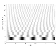
Figure 1: Evolution ($gt$) of the concurrence for initially unexcited $a$ and $b$ atoms and the field in a $n$ Fock state. Black means value $1$, maximum entanglement, white means value zero, and greys mean partial values of entanglement.

In the next section we study how the concurrence is affected by the presence of an effective atomic environment when only one excitation is involved.

III Effective Hamiltonian description

We consider a collection of $A+2$ non-identical two-level atoms interacting with a single mode of a quantized field in an ideal cavity. Two atoms, labelled by subindexes $a$ and $b$, are resonant with the mode whereas the other $A$ atoms interact dispersively with the mode. The Hamiltonian which drives the unitary dynamics of the whole system under the rotating wave approximation has the form

$$H = \omega_{f}a^{\dagger}a+\sum_{i=a,b}\omega_{i}s_{zi}+\sum_{j=1}^{A}\omega_{j}s_{zj}$$ (5)

$$+\sum_{j=a,b,1}^{A}g_{j}(as_{+j}+a^{\dagger}s_{-j}),$$

where $a^{\dagger}$ and $a$ are the usual one mode field operators, and $s_{z,\pm j}$ are the $z$ components of the Pauli operators corresponding to the $j-$th two-level atom ($j=a,b,1,\ldots,A$). Atomic operators obey the standard $SU(2)$ commutation relations, $[s_{+i},s_{-j}]=2s_{zi}\delta_{ij}$ and $[s_{zi},s_{\pm j}]=\pm s_{\pm i}\delta_{ij}$. Since the total number of excitations, represented by the operator $\hat{N}=a^{\dagger}a+\sum_{j=a,b,1}^{A}s_{zj}$, is an integral of motion, the above Hamiltonian can be rewritten as follows:

$$H=\omega_{f}\hat{N}+H_{int},$$ (6)

with

$$H_{int} = \sum_{j=1}^{A}\Delta_{j}s_{zj}+\sum_{i=a,b}g_{i}(as_{+i}+a^{\dagger}s_{-i})$$ (7)

$$+\sum_{j=1}^{A}g_{j}(as_{+j}+a^{\dagger}s_{-j}),$$

where $\Delta_{k}=\omega_{k}-\omega_{f}$, $k=1,\ldots,A$ are the detunings between the transition of the $k$th atom and the mode frequency. Now, we assume that all $A$ atoms are far from the resonance, so that $\Delta_{j}\gg g_{j}$, $j=1,2,\ldots,A$. The effective Hamiltonian, approximately describing the interaction process, can be obtained from the interaction Hamiltonian (7) by using the method of Lie rotations Small ; Sainz , namely by applying to the Hamiltonian (5) the following unitary transformation

$$V=e^{\hat{B}},\hskip 14.45377pt\hat{B}=\sum_{j=1}^{A}\epsilon_{j}(as_{+j}-a^{\dagger}s_{-j}),$$ (8)

where $\epsilon_{j}=g_{j}/\Delta_{j}\ll 1$. Neglecting terms of order higher than $\epsilon_{j}^{2}$, we obtain the following effective Hamiltonian:

$$H_{eff}=\sum_{j=1}^{A}(\Delta_{j}+g_{j}\epsilon_{j}(1+2a^{\dagger}a))s_{zj}+\hat{\lambda}\sum_{i=a,b}g_{i}(as_{+i}+a^{\dagger}s_{-i})+\frac{1}{2}\sum_{j,i=1}^{A}g_{i}\epsilon_{j}(s_{-i}s_{+j}+s_{+i}s_{-j}),$$ (9)

where we have defined the operator $\hat{\lambda}=1+\sum_{j=1}^{A}\epsilon_{j}^{2}s_{zj}$.

The last term in (9) represents an effective dipolar interaction between the non-resonant atoms, and its contribution to the system dynamics strongly depends on the internal resonance condition between atomic frequencies. Let us consider randomly distributed frequencies, such that they satisfy the condition $\Delta_{j}-\Delta_{i}\gg g$, $i,j=1,2,..A$. Then, the terms $i\neq j$ in the last sum of the effective Hamiltonian (9) rapidly oscillate and can be neglected. Finally, the effective Hamiltonian, up to a constant energy shift, becomes:

$$H_{eff} = \sum_{j=1}^{A}\Delta_{j}s_{zj}+(1+2a^{\dagger}a)\sum_{j=1}^{A}g_{j}\epsilon_{j}s_{zj}$$

$$+\hat{\lambda}\sum_{i=a,b}g_{i}(as_{+i}+a^{\dagger}s_{-i}).$$

In the given approximation the total number of excitations “stored”in the non-resonant atoms is a constant of motion, which reflects a dispersive character of interaction. The first term in the above equation represents just transition frequency shifts of the non-resonant atoms, and commutes with the rest of the terms (so, it can be taken out of the Hamiltonian). The second term is the dynamic Stark shift and its contribution to the resonant dynamics, described by the last term, strongly depends on the state of the non-resonant atoms, which can be considered as a kind of atomic environment.

Since the maximum entanglement in the system of two resonant atoms is reached when the total number of excitation is one, $N=1$, we consider exclusively this situation. So, under the constraint that there is only one photon, the corresponding evolution operator can be found and, in the standard tensor product basis, it is given by

$$U(t)=\left[\begin{array}[]{cccc}e^{i\hat{y}t/2}\hat{A}_{n+1}&-ig\hat{\lambda}a\hat{L}_{n}e^{i\hat{y}t/2}&-ig\hat{\lambda}a\hat{L}_{n}e^{i\hat{y}t/2}&0\\ -ig\hat{\lambda}a^{\dagger}\hat{L}_{n+1}e^{i\hat{y}t/2}&\hat{Y}_{n}&\hat{Y}_{n}-1&-ig\hat{\lambda}a\hat{L}_{n}e^{-i\hat{y}t/2}\\ -ig\hat{\lambda}a^{\dagger}\hat{L}_{n+1}e^{i\hat{y}t/2}&\hat{Y}_{n}-1&\hat{Y}_{n}&-ig\hat{\lambda}a\hat{L}_{n}e^{-i\hat{y}t/2}\\ 0&-ig\hat{\lambda}a^{\dagger}\hat{L}_{n+1}e^{-i\hat{y}t/2}&-ig\hat{\lambda}a^{\dagger}\hat{L}_{n+1}e^{-i\hat{y}t/2}&e^{-i\hat{y}t/2}\hat{A}_{n}^{\ast}\end{array}\right],$$ (10)

where we have defined the operators:

$$\hat{L}_{n} = \frac{\sin\hat{\Omega}_{n}t}{\hat{\Omega}_{n}}$$

$$\hat{Y}_{n} = \frac{1}{2}(e^{i\hat{y}t/2}\hat{A}_{n}^{\ast}+e^{-i\hat{y}t/2}\hat{A}_{n+1})$$

$$\hat{A}_{n} = \cos\hat{\Omega}_{n}t+i\frac{\hat{y}}{2}\hat{L}_{n},$$

and the Rabi frequencies $\hat{\Omega}_{n}$ depend on the field and on the environment variables as follows:

$$\hat{\Omega}_{n}=\left[\left(\frac{\hat{y}}{2}\right)^{2}+2g^{2}\hat{\lambda}^{2}\hat{n}\right]^{1/2},\quad\frac{\hat{y}}{2}=\sum_{j=1}^{A}g_{j}\epsilon_{j}s_{zj}.$$

So, the dynamics depends on the distribution of the different Rabi frequencies which appear as a contribution of $A$ non-resonance distinguishable two-level atoms and it also depends on the initial state of the whole system.

IV Evolution of the Entanglement

Now, let us suppose that the environment atoms are prepared in a coherent superposition of excited and ground states:

$$|\Psi_{0}\rangle_{env}=\prod{j=1}^{A}\frac{|0\rangle_{j}+|1\rangle_{j}}{\sqrt{2}}\frac{1}{2^{A/2}}\sum_{s_{1}}\sum_{s_{2}}\ldots\sum_{s_{A}}|s_{1}+1/2\rangle_{1}|s_{2}+1/2\rangle_{2}\ldots|s_{A}+1/2\rangle_{A},$$ (11)

where the last sum is taken over all possible binary vectors $\vec{s}=\left\{s_{1},s_{2},\ldots s_{A}\right\}$, $s_{j}=s_{zj}=\pm 1/2$. We capture the key features of the concurrence evolution by considering two particular cases of initial conditions. First, we suppose that the resonance atoms are initially in the ground state and that the field is in the one photon Fock state:

$$|\Psi\rangle=|0\rangle_{a}|0\rangle_{b}|1\rangle_{f}|\Psi_{0}\rangle_{env}.$$ (12)

Applying the evolution operator (10) to the (12) state and tracing up over the field and the off-resonance atomic environment, we obtain for the resonant atoms the following reduced density operator:

$$\rho_{ab}=\frac{1}{2^{A}}\sum_{m=1}^{2^{A}}\{\sin^{2}(\Omega_{1}^{(m)}t)|\psi^{+}\rangle_{ab\hskip 2.168ptab}\langle\psi^{+}|+\cos^{2}(\Omega_{1}^{(m)}t)|0\rangle_{a}|0\rangle_{b\hskip 2.168pta}\langle 0|_{b}\langle 0|\},$$ (13)

with

$$\Omega_{1}^{(m)} = \frac{\tilde{g}^{2}}{4}(\overrightarrow{\epsilon}\cdot\vec{s}^{(m)})^{2}=\frac{\tilde{g}^{2}}{4}(\sum_{j=1}^{A}\epsilon_{j}s_{j}^{(m)})^{2},$$ (14)

$$\lambda_{m} = 1+(\overrightarrow{\epsilon}^{2}\cdot\vec{s}^{(m)})=1+\sum_{j=1}^{A}\epsilon_{j}^{2}s_{j}^{(m)},$$ (15)

where $\vec{s}^{(m)}$ is a certain arrangement of the $\vec{s}$ vector and $s_{j}^{(m)}=\pm 1/2$. We have neglected order corrections higher than or equal to $\epsilon$ on the amplitudes. From now on the coupling constants for field-environment atoms are taken to be equal, $g_{j}=\tilde{g}$ for all $j$.

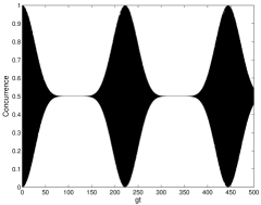
Figure 2: Evolution of the concurrence for initially unexcited $a$ and $b$ atoms and the field in the one-photon Fock state, with $A=7$, $\tilde{g}/g=1$, and $\tilde{g}/\bar{\Delta}=0.1$.

The concurrence corresponding to the density matrix (13) takes the form

$$\mathfrak{C}(\rho_{ab})=\frac{1}{2^{A}}\sum_{m=1}^{2^{A}}\sin^{2}(\Omega_{1}^{(m)}t).$$ (16)

If the resonant atoms are initially prepared in the symmetric one excitation state and the field is in the vacuum Fock state, then the initial state of the whole system is the following tensor product:

$$|\Psi\rangle=\frac{|0\rangle_{a}|1\rangle_{b}+|1\rangle_{a}|0\rangle_{b}}{\sqrt{2}}|0\rangle_{f}|\Psi_{0}\rangle_{env}.$$ (17)

In a similar way as described in the previous case (12) the concurrence takes the form

$$\mathfrak{C}(\rho_{ab})=\frac{1}{2^{A}}\sum_{m=1}^{2^{A}}\cos^{2}(\Omega_{1}^{(m)}t).$$ (18)

It is worth noting that the concurrences (16,18) are composed of many Rabi frequencies, which leads to a structure similar to the collapses and revivals in the Jaynes-Cummings model Tavis ; Banacloche . Nevertheless, in the present case the set of different frequencies is due to the presence of the dispersive atomic environment in contrast to the standard JCM where different Rabi frequencies appear as contributions of different Fock field states (recall that a well-defined collapse-revival structure requires a significant number of excitations Banacloche ; Retamal ).

Let us consider randomly distributed numbers $\Delta_{j}$, $j=1,\ldots,A$ with the mean $\bar{\Delta}$ and the standard deviation $\sigma_{\Delta}$. Then, the numbers $\epsilon_{j}$, $\epsilon_{j}^{2}$ have the following mean values and standard deviations:

$$\bar{\epsilon} \approx \frac{\tilde{g}}{\bar{\Delta}}\left(1+\frac{\sigma_{\Delta}^{2}}{\bar{\Delta}^{2}}\right),\hskip 23.84923pt\sigma_{\epsilon}\approx\frac{\tilde{g}\sigma_{\Delta}}{\bar{\Delta}^{2}},$$ (19)

$$\overline{\epsilon^{2}} \approx \frac{\tilde{g}^{2}}{\bar{\Delta}^{2}}\left(1+\frac{3\sigma_{\Delta}^{2}}{\bar{\Delta}^{2}}\right),\hskip 10.84006pt\sigma_{\epsilon^{2}}\approx\frac{2\tilde{g}^{2}\sigma_{\Delta}}{\bar{\Delta}^{3}}.$$ (20)

First, we will find the distribution of the (14) quantities. We assume that $\sigma_{\epsilon}\ll\bar{\epsilon}$ and $\sigma_{\epsilon^{2}}\ll\overline{\epsilon^{2}}$. Then, there are $A+1$ peaks corresponding to different values of the number of positive components of $\vec{s}$, $k=0,\ldots A$; for a given value of $k$ there are $C_{k}^{A}=A!/[k!(A-k)!]$ values of $(\vec{\epsilon}\cdot\vec{s})$ and $(\overrightarrow{\epsilon^{2}}\cdot\vec{s})$ which are normally distributed in accordance with the central limit theorem. For the $k$th peak, the mean value and the standard deviation are given by

$$\langle(\vec{\epsilon}\cdot\vec{s})\rangle_{k} = (k-A/2)\bar{\epsilon},\hskip 17.34518pt\sigma_{\epsilon,k}=\sigma_{\epsilon}\sqrt{\frac{k(A-k)}{A-1}},$$

$$\langle(\overrightarrow{\epsilon^{2}}\cdot\vec{s})\rangle_{k} = (k-A/2)\overline{\epsilon^{2}},\hskip 8.67204pt\sigma_{\epsilon^{2},k}=\sigma_{\epsilon^{2}}\sqrt{\frac{k(A-k)}{A-1}}.$$

Note that the first and the last peaks are infinitely narrow.

The Rabi frequency distribution has $A+1$ peaks (now the summation in (16, 18) is from $k=0$ to $A$), and the frequency corresponding to the $k$th peak can be approximated as follows:

$$\Omega_{k}\approx\sqrt{2}g[1+\frac{\tilde{g}^{2}}{\bar{\Delta}^{2}}(k-\frac{A}{2})(1+\frac{\tilde{g}^{2}}{4g^{2}}(k-\frac{A}{2}))].$$

Thus, the expressions (16) and (18) for the concurrence can be approximated as follows:

$$\mathfrak{C}(\rho_{ab})\approx\frac{1}{2}\left[1\pm\frac{1}{2^{A}}\text{Re}\sum_{k=0}^{A}C_{k}^{A}\exp(2i\Omega_{k}t)\right].$$ (21)

The $d_{k}$ separation between the $k$th and the $(k+1)$th peaks, and the $\delta_{k}$ width of the $k$th peak are

$$d_{k} = \sqrt{2}g[\frac{\tilde{g}^{2}}{\bar{\Delta}^{2}}+\frac{\tilde{g}^{4}}{4g^{2}\bar{\Delta}^{2}}(2k-A+1)],$$

$$\delta_{k} = \sqrt{2}g[1+(k-\frac{A}{2})+\frac{\tilde{g}^{2}}{4g^{2}}(k-\frac{A}{2})^{2}]\sigma_{\epsilon^{2},k}.$$

Then, considering the approximation of narrow peaks, $\delta_{k}\ll d_{k}$, i.e. $\sigma_{\Delta}\ll\bar{\Delta}/\sqrt{A}$, the sum in (21) can be represented as a sum of Gaussians, that is

$$\mathfrak{C}(\rho_{ab})\approx\frac{1}{2}\pm\frac{\bar{\Delta}^{2}e^{2\sqrt{2}igt}}{2\tilde{g}^{2}\sqrt{2A}\sigma}\text{Re}\sum_{k=-\infty}^{\infty}e^{-\frac{\left(gt-\frac{\pi k\bar{\Delta}^{2}}{\sqrt{2}\tilde{g}^{2}}\right)^{2}}{2\sigma^{2}}},$$ (22)

with the width

$$\sigma^{2}=\frac{\bar{\Delta}^{4}}{2\tilde{g}^{4}A}-it\frac{\sqrt{2}\bar{\Delta}^{2}}{8g},$$ (23)

which grows with time. The (22) sum reveals the collapse-revival structure of the concurrences (16) and (18). The first collapse happens when

$$gt_{c}\sim\frac{\bar{\Delta}^{2}}{\sqrt{A}\tilde{g}^{2}},$$ (24)

and it is followed by revival at time:

$$gt_{R}\sim\pi k\frac{\bar{\Delta}^{2}}{\sqrt{2}\tilde{g}^{2}},\hskip 14.45377ptk=1,2,....$$ (25)

In Figure 2 we show the exact evolution of the concurrence for initially unexcited atoms and the field in the one-photon Fock state in the presence of the environment atoms. One can observe that the entanglement also reaches its maximum value. We can estimate from (24) and (25) the time scale required to observe the environment induced collapse-revival structure. Taking the typical values of the interaction constant from Haroshe : $g/2\pi=24kHz$ and $\bar{\Delta}/2\pi\sim 70kHz$, we obtain $t_{R}\sim 100\mu s$ which is of order of the passage time of the atom through the cavity (cold atoms, $v\sim 100m/s$) and less than the photon lifetime $\sim 160\mu s$. The collapse time is $\sqrt{A}$ times less than $t_{R}$.

V Conclusions

In summary, we have studied the dynamics of the concurrence of two atoms resonantly interacting with a cavity mode in the presence of many off-resonance atoms. We have shown that, for random distribution of atomic detunings and initially symmetric excitation of non-resonant atoms, the coherent influence of the environment can be separated from the dephasing. The coherence influence of the environment reflects in the appearance of the collapse-revival structure of the concurrence, with an average value of one half. This behavior is induced only by the presence of the dispersive environment. It is worth noting that the entanglement of formation in revival periods has as extreme value $1$, which means that the state of the bipartite system becomes pure at those times.

- (1) P. W. Shor, Phys. Rev. A 52, 2493 (1995); D. P. DiVicenzo, Science 270, 255 (1995); L. K. Grover, Phys. Rev. Lett. 79, 325 (1997); J. I. Cirac, P. Zoller, Nature 404, 579 (2000).
- (2) M. A. Nielsen and I. L. Chuang, Quantum Computation and Quantum Information (Cambridge University Press, Cambridge, 2000); G. Alber et al., Quantum Information (Springer, Berlin, 2001); D. Bouwmeester, A. Ekert, and A. Zeilinger, The Physics of Quantum Information (Spring-Verlag, Berlin/Heidelberg/New York, 2000); Asher Peres Quantum Theory: Concepts and Methods (Kluwer Academic Publishers, Dordrecht/Boston/London, 1998).
- (3) A. K. Ekert, Phys. Rev. Lett. 67, 661 (1991).
- (4) D. Deutsch and R. Jozsa, Proc. R. Soc. London A 439, 553 (1992).
- (5) C. H. Bennett, G. Brassard, C. Crépeau, R. Jozsa, A. Peres, and W. Wootters, Phys. Rev. Lett. 70, 1895 (1993).
- (6) X. X. Yi, C. S. Yu, L. Zhou, and H. S. Song, Phys. Rev. A 68, 052304 (2003).
- (7) M. B. Plenio, S. F. Huelga, A. Beige and P. L. Knight, Phys. Rev. A 59, 2468 (1999); T. A. Costi and R. H. McKenzie, Phys. Rev. A 68, 034301 (2003); S. B. Li and J. B. Xu, quantum-ph/0505216.
- (8) J. H. An, S. J. Wang and H. G. Luo, J. Phys. A: Math. Gen. 38, 3579 (2005).
- (9) B. Kraus, J. I. Cirac, Phys. Rev. Lett. 92, 013602 (2004).
- (10) M. G. Benedict, P. Földi, A. Czirják and T. Serényi, J. Opt. B: Quant. Semm. 6, S3-S6 (2004).
- (11) S. Schneider and G. J. Milburn, Phys. Rev. A 65, 042107 (2002).
- (12) S. Ishizaka, Phys. Rev. A 63, 034301 (2001); S. Paganelli, F. de Pasquale and S. M. Giampaolo, Phys. Rev. A 66, 052317 (2002); C. Pineda, T. H. Seligman, quantum-ph/0503177 (2005); Z. Gedik, quantum-ph/0505176.
- (13) C. M. Dawson, A. P. Hines, R. H. McKenzie and G. J. Milburn, Phys. Rev. A 71, 052321 (2005).
- (14) M. Lucamarini, S. Paganelli and S. Mancini, Phys. Rev. A 69, 062308 (2004).
- (15) X. S. Ma, A. M. Wang, X. D. Yang, and H. You, J. Phys A: Math. Gen. 38, 2761 (2005).
- (16) D. Braun, Phys. Rev. Lett. 89, 277901 (2002).
- (17) F. Benatti, R. Floreanini and M. Piani, Phys. Rev. Lett. 91, 070402 (2003).
- (18) M. B. Plenio and S. F. Huelga, Phys. Rev. Lett. 88, 197901 (2002).
- (19) Y. Gao and S. J. Xiong, Phys. Rev. A 71, 034102 (2005).
- (20) K. Aoi, H. Deuling, and K. H. Bennemann, Phys. Rev. B 10, 1975 (1974).
- (21) S. B. Zheng and G. C. Guo, Phys. Rev. Lett. 85, 2392 (2000).
- (22) T. E. Tessier, I. H. Deutsch, A. Delgado, and I. Fuentes-Guridi, Phys. Rev. A 68, 062316 (2003); M. S. Kim, J. Lee, D. Ahn and P. L. Knight, Phys. Rev. A 65, 040101 (2002); S. B. Li and J. B. Xu, quant-ph/0507072.
- (23) Z. Ficek and R. Tanas, J. Mod. Opt. 50, 18, 2765-2779, (2003).
- (24) M. Tavis and F. W. Cummings, Phys. Rev. 170, 379 (1968).
- (25) M. Brune et al., Phys. Rev. Lett. 77, 4887 (1996).
- (26) W. H. Zurek, F. M. Cucchietti, and J. P. Paz, quant-ph/0312207; F. M. Cucchietti, J. P. Paz, and W. H. Zurek, quant-ph/0508184.
- (27) K. Molmer and Sorensen, Phys. Rev. Lett. 82, 1835 (1999).
- (28) A. B. Klimov and L. L. Sanchez-Soto, Phys. Rev. A 61, 063802 (2000).
- (29) I. Sainz, A. B. Klimov and S. M. Chumakov, J. Opt. B: Quan. Semm. Opt. 5, 190 (2003).
- (30) W. K. Wootters, Phys. Rev. Lett. 80, 2245 (1998).
- (31) N. B. Narozhny, J. J. Sanchez-Mondragon and J. H. Eberly, Phys. Rev. A 23, 236 (1981).
- (32) J. Gea-Banacloche, Phys. Rev. Lett. 65, 3385 (1990).
- (33) J. C. Retamal, C. Saavedra, A. B. Klimov, and M. Chumakov, Phys. Rev. A 55, 2413 (1997).