Quantum measurement of a mesoscopic spin ensemble

Abstract

We describe a method for precise estimation of the polarization of a mesoscopic spin ensemble by using its coupling to a single two-level system. Our approach requires a minimal number of measurements on the two-level system for a given measurement precision. We consider the application of this method to the case of nuclear spin ensemble defined by a single electron-charged quantum dot: we show that decreasing the electron spin dephasing due to nuclei and increasing the fidelity of nuclear-spin-based quantum memory could be within the reach of present day experiments.

I Introduction

Decoherence of quantum systems induced by interactions with low-frequency reservoirs is endemic in solid-state quantum information processing (QIP) Johnson et al. (2005); Ithier et al. (2005). A frequently encountered scenario is the coupling of a two-level system (qubit) to a mesoscopic bath of two-level systems such as defects or background spins. The manifestly non-Markovian nature of system-reservoir coupling in this scenario presents challenges for the description of the long term dynamics as well as for fault tolerant quantum error correction Alicki et al. (2002); Terhal and Burkard (2005). The primary experimental signature of a low-frequency reservoir is an unknown but slowly changing effective field that can substantially reduce the ability to predict the system dynamics. A possible strategy to mitigate this effect is to carry out a quantum measurement which allows for an estimation of the unknown reservoir field by controlled manipulation and measurement of the qubit. A precise estimation of the field acting on the large Hilbert space of the reservoir requires, however, many repetitions of the procedure: this constitutes a major limitation since in almost all cases of interest projective measurements on the qubit are slow Elzerman et al. (2004) and in turn will limit the accuracy of the estimation that can be achieved before the reservoir field changes.

In this work, we propose a method for estimating an unknown quantum field associated with a mesoscopic spin ensemble. By using an incoherent version of the quantum phase estimation algorithm, Kitaev (1995); Nielsen and Chuang (2000) we show that the number of qubit measurements scale linearly with the number of significant digits of the estimation. We only assume the availability of single qubit operations such as preparation of a known qubit state, rotations in the $xy$-plane, and measurement, of which only rotations need to be fast. The estimation procedure that we describe would suppress the dephasing of the qubit induced by the reservoir; indeed, an interaction with the estimated field leads to coherent unitary evolution that could be used for quantum control of the qubit. If the measurement of the reservoir observable is sufficiently fast and strong, it may in turn suppress the free evolution of the reservoir in a way that is reminiscent of a quantum Zeno effect.

After presenting a detailed description of the measurement procedure and discussing its performance and limitations, we focus on a specific application of the procedure for the case of a single quantum dot (QD) electron spin interacting with the mesoscopic nuclear spin ensemble defined by the QD. It is by now well known that the major source of decoherence for the electron-spin qubits in QDs Loss and DiVincenzo (1998) is the hyperfine interaction between the spins of the lattice nuclei and the electron Khaetskii et al. (2002); Merkulov et al. (2002); Schliemann et al. (2003); Coish and Loss (2004); Erlingsson and Nazarov (2004); de Sousa et al. (2005); Deng and Hu (2005). A particular feature of the hyperfine-related dephasing is the long correlation time ($t_{c}$) associated with nuclear spins. This enables techniques such as spin-echo to greatly suppress the dephasing Petta et al. (2005). In Coish and Loss (2004) it was suggested to measure the nuclear field to reduce electron spin decoherence times; precise knowledge of the instantaneous value of the field would even allow for controlled unitary operations. For example, knowledge of the field in adjacent QDs yields an effective field gradient that could be used in recently proposed quantum computing approaches with pairs of electron spins Taylor et al. (2005). Moreover, with sufficient control, the collective spin of the nuclei in a QD may be used as a highly coherent qubit-implementation in its own right Taylor et al. (2003a, b, 2004).

II Phase estimation

In the following we consider an indirect measurement scheme in which the system under investigation is brought into interaction with a probe spin (a two-level system in our case) in a suitably prepared state. Measuring the probe spin after a given interaction time $t$ yields information about the state of the system. We assume the mesoscopic system evolves only slowly compared to the procedure, and further that the measurement does not directly perturb the system. In essence, we are performing a series of quantum non-demolition (QND) measurements on the system with the probe spin.

We consider an interaction Hamiltonian of the form

$$H_{\mathrm{int}}=\hbar A_{z}\otimes S_{z}$$ (1)

which lends itself easily to a measurement of the observable $A_{z}$. The QND requirement is satisfied for $[H_{\rm int},H_{\rm bath}]\rightarrow 0$. The applicability of $H_{\mathrm{int}}$ in situations of physical interest is discussed in Sec. VI. Given this interaction, the strategy to measure $A_{z}$ is in close analogy to the so-called Ramsey interferometry approach, which we now briefly review.

For example, an atomic transition has a fixed, scalar value for $A_{z}$ which corresponds to the transition frequency. By measuring $A_{z}$ as well as possible in a given time period, the measurement apparatus can be locked to the fixed value, as happens in atomic clocks. The probe spin $S$ is prepared in a state $\left|+\right>=(\left|\uparrow\right>+\left|\downarrow\right>)/\sqrt{2}$. It will undergo evolution under $H$ according to $U_{t}=\exp(-itA_{z}S_{z})$. After an interaction time $t$, the probe spin’s state will be

$$\cos(\Omega t)\left|+\right>+i\sin(\Omega t)\left|-\right>$$ (2)

where $\Omega=A_{z}/2$ is the precession frequency for the probe spin. A measurement of the spin in the $\left|\pm\right>$ basis yields a probability $\cos^{2}(\Omega t)$ of being in the $\left|+\right>$ state. Accumulating the results of many such measurements allows one to estimate the value for $\Omega$ (and therefore $A_{z}$). In general, the best estimate is limited by interaction time: for an expected uncertainty in $A_{z}$ of $\Delta_{0}$ and an appropriate choice of $t$, $M$ measurements with fixed interaction times $1/\Delta_{0}$ can estimate $A_{z}$ to no better than $\sim\Delta_{0}/\sqrt{M}$ (see Wineland et al. (1992) and references therein).

In our scenario, the situation is slightly different in that $A_{z}$ is now a quantum variable. For a state $\left|s\right>$ in the Hilbert space of the system $\mathcal{H}$ which is an eigenstate of $A_{z}$ with eigenvalue $2\Omega_{s}$, the coupling induces oscillations:

$$U_{t}\left|s\right>\left|+\right>=\left|s\right>\left[\cos(\Omega_{s}t)\left|+\right>+i\sin(\Omega_{s}t)\left|-\right>\right]\ .$$ (3)

Thus, the probability to measure the probe spin in state $\left|+\right>$ given that the system is in a state $\left|s\right>$ is $p(+|s)=\cos^{2}(\Omega_{s}t)$ at time $t$, providing information about which eigenvalue of $A_{z}$ is realized. Comparing Eq. (2) to Eq. (3) indicates that the same techniques used in atomic clocks (Ramsey interferometry) could be used in this scenario to measure $\Omega_{s}$ and thus project the bath in some eigenstate of $A_{z}$ with an eigenvalue of $\Omega_{s}$ to within the uncertainty of the measurement.

Beyond the Ramsey approach, there are several ways to extract this information, which differ in the choice of interaction times $t_{j}$ and the subsequent measurements. The general results on quantum metrology of Giovannetti et al. (2006) show, however, that the standard Ramsey scheme with fixed interaction time $t$ is already optimal in that the scaling of the final variance with the inverse of the total interaction time cannot be improved without using entangled probe states. Nevertheless, the Ramsey scheme will not be the most suitable in all circumstances. For example, we have assumed so far that preparation and measurement of the probe spin is fast when compared to $1/\Delta_{0}$. However, in many situations with single quantum systems, this assumption is no longer true, and it then becomes desirable to minimize the number of preparation/measurement steps in the scheme.

III The measurement scheme

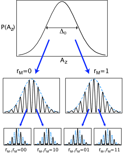
Figure 1: (Color online) Illustration of the first two steps of the measurement procedure. The original distribution $P(A_{z})$, with rms width $\Delta_{0}$ is shown at the top. After the first measurement, with result $r_{M}=0,1$, the conditional distribution (middle plots) reflects the knowledge of the least significant bit. The next measurement result $r_{M-1}$ further reduces the distribution (bottom plots).

We now show that by varying the interaction time and the final measurements such that each step yields the maximum information about $\Omega_{s}$, we can obtain the same accuracy as standard Ramsey techniques with a similar interaction time, but only a logarithmic number of probe spin preparations and measurements. As a trivial case, if $A_{z}$ had eigenvalues $0$ and $1$ only, then measuring the probe in the $\pm$-basis after an interaction time $t_{1}=\pi$, we find $+(-)$ with certainty, if the system are in an $A_{z}=0(1)$-eigenstate; if they were initially in a superposition, measuring the probe projects the system to the corresponding eigenspaces. We can extend this simple example (in the spirit of the quantum phase estimation algorithm Kitaev (1995); Nielsen and Chuang (2000) and its application to the measurement of a classical field Vaidman and Mitrani (2004)) to implement an $A_{z}$-measurement by successively determining the binary digits of the eigenvalue. We start with the ideal case, then generalize to a more realistic scenario.

III.1 Ideal case

If all the eigenvalues of $A_{z}$ are an integer multiple of some known number $\alpha$ and bounded by $2^{M}\alpha$, then this procedure yields a perfect $A_{z}$-measurement in $M$ steps: let us write all eigenvalues as $2\Omega_{s}=\alpha 2^{M}\sum_{l=1}^{M}s_{l}2^{-l}$. The sum we denote by $s$ and also use the notation $s=0.s_{1}s_{2}\dots s_{M}$. Starting now with an interaction time $t_{1}=\frac{\pi}{\alpha}$, we have $\Omega_{s}t_{1}=s_{M}\frac{\pi}{2}\,\mathrm{mod}\,\pi$. Hence the state of the probe electron is flipped if and only if $s_{M}=1$. Therefore measuring the probe electron in state $+(-)$ projects the nuclei to the subspace of even(odd) multiples of $\alpha$ (see Fig. 1). We denote the result of the first measurement by $r_{M}=0(1)$ if the outcome was “$+(-)$”. All the higher digits have no effect on the measurement result since they induce rotations by an integer multiple of $\pi$ which have no effect on the probabilities $p(\pm|s)$.

To measure the higher digits, we reduce the interaction time by half in each subsequent step: $t_{j+1}=2^{-j}t_{1}$ until we reach $t_{M}=\frac{\pi}{\alpha}$ in the final and shortest step. For $j>1$ the rotation angle $\Omega_{s}t_{j}$ (mod $\pi$) in the $j$th step does not only depend on the $j$th binary digit of $s$ but also on the previous digits (which have already been measured, giving results $r_{M+1-l}=s_{M+1-l},l=1,\dots,j-1$). The angle $\Omega_{s}t_{j}$ (mod $\pi$) is given by $s_{M+1-j}\frac{\pi}{2}+\varphi_{j}$ with $\varphi_{j}=\frac{\pi}{2}\sum_{l=1}^{j-1}r_{M+1-l}2^{l-j}$, where we have used the results $r_{l}$ already obtained. This over-rotation by the angle $\varphi_{j}$ can be taken into account in the choice of the measurement basis for the $j$th step: if the $j$th measurement is performed in a rotated basis $\left|\pm_{j}\right>$ that is determined by the previous results $r_{l}$, namely

$$\left|+_{j}\right> \mathrel{\raise 0.40903pt\hbox{:}\mkern-4.2mu=} \cos\varphi_{j}\left|+\right>-i\sin\varphi_{j}\left|-\right>,$$ (4a)

$$\left|-_{j}\right> \mathrel{\raise 0.40903pt\hbox{:}\mkern-4.2mu=} \sin\varphi_{j}\left|+\right>+i\cos\varphi_{j}\left|-\right>,$$ (4b)

then the $j$th measurement yields “$+$” ($r_{M+1-j}=0$) if $s_{M+1-j}=0$ and “$-$” ($r_{M+1-j}=1$) otherwise. Thus, after $M$ measurements we obtain $r_{l}=s_{l},\forall l=1,\dots,M$ and have performed a complete measurement of $A_{z}$ (where the number $M$ of probe particles used is the smallest integer such that $2^{M}\geq A_{z}/\alpha$).

Before proceeding, we note that the proposed scheme is nothing but an “incoherent” implementation of the quantum phase estimation algorithm: As originally proposed, this algorithm allows measurement of the eigenvalue of a unitary $U$ by preparing $M$ qubits (the control-register) in the state $\left|+\right>^{\otimes M}$ (i.e., the equal superposition of all computational basis states $\left|j\right>,j=0,\dots,2^{M}-1$) and performing controlled-$U^{2^{j-1}}$ gates between the $j$th qubit and an additional register prepared in an eigenstate $\left|s\right>$ of $U$ with $U\left|s\right>=e^{i2\pi s}\left|s\right>$. The controlled-$U$ gates let each computational basis state acquire a $s$-dependent phase: $\left|l\right>\mapsto e^{i2\pi ls}\left|l\right>$. Then the inverse quantum Fourier transformation (QFT) is performed on the control register, which is then measured in the computational basis, yielding the binary digits of $s$. Performing the QFT is still a forbidding task, but not necessary here: the sequence of measurements in the rotated basis $\left|\pm_{j}\right>$ described above is in fact an implementation of the combination of QFT and measurement into one step. This was previously suggested in different contexts Griffiths and Niu (1996); Parker and Plenio (2000); Tomita and Nakamura (2004).

III.2 Realistic case

In general, there is no known $\alpha$ such that all eigenvalues $s$ of $A_{z}$ are integer multiples of $\alpha$. Nevertheless, as discussed below, the above procedure can still produce a very accurate measurement of $A_{z}$ if sufficiently many digits are measured. Now we evaluate the performance of the proposed measurement scheme in the realistic case of non-integer eigenvalues. Since here we are interested in the fundamental limits of the scheme, we will for now assume all operations on the probe qubit (state preparation, measurement, and timing) to be exact; the effect of these imperfection is considered in Sec. V. Without loss of generality, let $A$ and $0$ denote the largest and smallest eigenvalues of $A_{z}$, respectively and choose $\alpha=2A$ such that the eigenvalues of $A_{z}/\alpha$ are all $\in[0,1/2]$. These are the eigenvalues $s$ we measure in the following.

The function from which all relevant properties of our strategy can be calculated is the conditional probability $p_{M}(R|s)$ to obtain (after measuring $M$ electrons) a result $R=0.r_{1}r_{2}\dots r_{M}$ given that the system was prepared in an eigenstate with eigenvalue $s$. The probability to measure $R$ is given by the product of the probabilities to measure $r_{M+1-j}$ in the $j$th step, which is $\cos^{2}(\Omega_{s}t_{j}-\varphi_{j}+r_{M+1-j}\frac{\pi}{2})=\cos^{2}(\pi[s-R]2^{M-j})$. Hence

$$p_{M}(R|s)=\prod_{k=0}^{M-1}\cos^{2}(\pi[s-R]2^{k}),$$ (5)

see also Vaidman and Mitrani (2004). This formula can be simplified by repeatedly using $2\sin x=\sin(x/2)\cos(x/2)$ to give

$$p_{M}(R|s)=\left(\frac{\sin(2^{M}\pi[s-R])}{2^{M}\sin(\pi[s-R])}\right)^{2}.$$ (6)

Assume the nuclei are initially prepared in a state $\rho$ with prior probability $p(s)$ to find them in the eigenspace belonging to the eigenvalue $s$. After the measurement, we can update this distribution given our measurement result. We obtain, according to Bayes’ formula:

$$p_{M}(s|R)=\frac{p_{M}(R|s)p(s)}{\sum_{s}p_{M}(R|s)p(s)},$$ (7)

with expectation value denoted by $\bar{s}_{R}$.

IV Performance of the scheme

As the figure of merit for the performance of the measurement scheme we take the improvement of the average uncertainty in $A_{z}$ of the updated distribution

$$\overline{\Delta A_{z,\mathrm{est}}}^{(M)}\mathrel{\raise 0.40903pt\hbox{:}\mkern-4.2mu=}\sum_{R}p_{M}(R)\sqrt{\sum_{s}(s-\bar{s}_{R})^{2}p_{M}(s|R)}$$ (8)

over the initial uncertainty $\Delta_{0}=\Delta A_{z}^{(0)}$. An upper bound to $\overline{\Delta A_{z,\mathrm{est}}}^{(M)}$ is given by the square root of the average variance $\overline{V}$

$$\overline{V}_{M}\mathrel{\raise 0.40903pt\hbox{:}\mkern-4.2mu=}\sum_{R}p_{M}(R)\sum_{s}(s-\bar{s}_{R})^{2}p_{M}(s|R),$$ (9)

as easily checked by the Cauchy-Schwarz inequality. We now show that $\overline{V}_{M}\leq 2^{-M}$. We replace $\bar{s}_{R}\to\tilde{R}=\mathrm{min}\{R,1-R\}$; we can use any such replacement to obtain an upper bound, as the expectation value $\bar{x}=\sum_{x}p(x)x$ minimizes $v(y)=\sum_{x}p(x)(x-y)^{2}$. This choice means that measurement results $R>1/2$ are interpreted as $1-R$, which is appropriate since the scheme does not distinguish the numbers $s=\delta$ and $s^{\prime}=1-\delta$ and due to the choice of $\alpha$ only $s\in[0,1/2]$ occur. Thus

$$\overline{V}_{M} \leq \sum_{s}p(s)\sum_{R}(s-\tilde{R})^{2}p_{M}(R|s)\mathrel{=\mkern-4.2mu\raise 0.40903pt\hbox{:}}\sum_{s}p(s)\overline{V}_{M}(s).$$

The terms $\overline{V}_{M}(s)$ can be shown to be $\leq b_{V}\,2^{-M}$ with $b_{V}=(1+2^{-M})/2$. This means that performing $M$ measurements yields a state with $A_{z}$-uncertainty $\Delta A_{z,\mathrm{est}}\leq\alpha 2^{-M/2}$. For example, we need about $13$ interactions with the probe spin to reach the $1\%$-level in $\Delta A_{z,\mathrm{est}}/\alpha$ and about $7$ more for every additional factor of $10$.

The overall procedure requires a total time $T_{M}=\sum_{j=1}^{M}(t_{j}+\tau_{m})=2t_{1}(1-2^{-M})+M\tau_{m}$, which is an interaction time (determined mainly by the time $t_{1}=\frac{\pi}{\alpha}2^{M}=\pi(2f\Delta_{0})^{-1}2^{M}$ needed for the least significant digit probed) and the time to make $M$ measurements ($\tau_{m}$ is the time to make a single measurement). We obtain for the average uncertainty an upper bound in terms of the interaction time $T_{\rm int}=T_{M}-M\tau_{m}$ needed:

$$\frac{\Delta A_{z,\mathrm{est}}}{\Delta_{0}}\leq\sqrt{\frac{\pi f}{\Delta_{0}T_{\mathrm{int}}}}.$$ (10)

Immediately the similarity with standard atomic clock approaches is apparent, as the uncertainty decreases with the square root of the interaction time. However, while for an atomic clock scheme, in which the interaction time per measurement is kept fixed to $\sim\pi/(f\Delta_{0})$, the total time to reach the precision of Eq. (10) is $T^{\rm r}_{M}=2t_{1}+\tau_{m}2^{M}$. For our method the measurement time is reduced dramatically by a time $T^{\rm r}_{M}-T_{M}=\tau_{m}(2^{M}-M)$. In this manner our approach requires a polynomial, rather than exponential, number of measurements for a given accuracy, though the overall interaction time is the same for both techniques.

It may be remarked that even the scaling in interaction time differs significantly if other figures of merit are considered. For example, our scheme provides a square-root speed-up in $T_{\mathrm{int}}$ over the standard Ramsey scheme if the aim is to maximize the information gain or to minimize the confidence interval Masanes et al. (2002).

V Errors and Fluctuations in $A_{z}$

Up until now we have considered an idealized situation in which the value of $A_{z}$ does not change over the course of the measurement and in which preparation and measurement of the probe system work with unit fidelity. Let us now investigate the robustness of our scheme in the presence of these errors.

V.1 Preparation and Measurement Errors

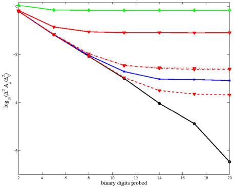
Figure 2: (Color online) Estimation in the presence of preparation and measurement error $p$: the logarithm of the improvement $\Delta A_{z,{\rm est}}/\Delta_{0}$ is plotted versus the number $M$ of binary digits measured. The solid lines represent different error rates ($p=0$: black circles; $p=10^{-4}$ blue crosses; $p=10^{-2}$: red triangles; and $p=10^{-1}$: green diamonds).
The broken red curves (triangles) demonstrate the benefit of simple error correction (for $p=10^{-2}$): strategy I (3 repetitions per digit, use majority result; either for all digits or only for leading $M/2$ digits): (dash-dotted, dotted – almost undistinguishable); strategy II (increase number of repetitions for more significant digits to 7 repetitions for leading $M/8$ digits, 5 for next $M/8$, and 3 for next $M/4$): dashed. We see that the latter provides a better accuracy than the uncorrected $p=10^{-4}$ curve.

By relying upon a small number of measurements, the scheme we described becomes more susceptible to preparation and measurement errors. An error in the determination of the $k$th digit leads to an increase of the error probability in the subsequent digits. This error amplification leads to a scaling of the final error of $\sqrt{p}$, where $p$ is the probability of incurring a preparation or measurement error in a single step. We confirm this with Monte Carlo simulations of the measurement procedure (Fig. 2a), leading to an asymptotic bound:

$$\Delta A_{z,\mathrm{est}}\leq(2f\Delta_{0})\sqrt{p}.$$ (11)

Standard error correction (EC) techniques can be used to overcome this problem. E.g., by performing three measurements for each digit and using majority vote, the effective probability of error can be reduced to $\sim 3p^{2}$ – at the expense of tripling the interaction time and number of measurements. While this may look like a big overhead, it should be noted that the scheme can be significantly improved: the least significant digits do not require any EC. For them, the scheme gives noisy results even for error rate $p=0$ due to the undetermined digits of $A_{z}$, this does not affect the most significant $M/2$ digits. This indicates that it may be enough to apply EC for the leading digits.

As can be seen from Fig. 2b, this simple EC strategy provides a significant improvement in the asymptotic $\Delta A_{z}$. This is hardly changed, when EC is applied only to the leading half of the digits. Thus only twice as many measurements (and an additional interaction time $\sim 2^{M/2+2}$ which is $\ll T_{M}$) is needed for an order-of-magnitude improvement in $\Delta A_{z}$. By repeating the measurement of more important digits even more often, the effect of technical errors can be reduced even further, as confirmed by Monte Carlo simulations (Fig. 2b). We also note that further improvements (beyond $M$ digits) can be achieved by this technique. In essence, choosing a digital approach to error correction for our digital technique yields substantially better performance than adapting the digital technique to an analog approach.

V.2 Estimation of bath decorrelation errors

In practice, internal bath dynamics will lead to fluctuations in $A_{z}$, such that $A_{z}(t)\neq A_{z}(t^{\prime})$ for times $t$ and $t^{\prime}$ that are sufficiently different. Furthermore, apparatus errors, as outlined above, lead to errors in our measurement procedure. We will assume that the variations of $A_{z}$ are slow over short time intervals, allowing us to approximate the $M$ bit measurement process as a continuous measurement over the time $T_{M}$ with some additional noise with variance $\approx\Delta A_{z,{\rm est}}(M)^{2}\ll\Delta_{0}^{2}$. Then we will find the expected difference in our measurement result and the value of $A_{z}$ at a later time.

Under the above approximations the value of the $k$th such measurement (where a complete set of $M$ bits takes a time $T_{M}$ and the $k$th such measurement ends at time $t_{k}$) is

$$m_{k}=\frac{1}{T_{M}}\int_{t_{k}-T_{M}}^{t_{k}}A_{z}(t)dt+G_{k}$$ (12)

where the noise from measurement is incorporated in the stochastic noise variable $G_{k}$ with $\langle G_{k}G_{k^{\prime}}\rangle\approx\delta_{kk^{\prime}}\Delta A_{z,{\rm est}}(M)^{2}$. We can estimate $A_{z}$ at a later time, and find the variance of this estimate from the actual value:

$$\bar{V}_{M}(t>t_{k}) = \langle[m_{k}-A_{z}(t)]^{2}\rangle$$

$$= \langle G_{k}^{2}\rangle+\Delta_{0}^{2}+\frac{1}{2T_{M}^{2}}\int_{t_{k}-T_{M}}^{t_{k}}\int_{t_{k}-T_{M}}^{t_{k}}\langle\{A_{z}(t^{\prime}),A_{z}(t^{\prime\prime})\}_{+}\rangle dt^{\prime\prime}dt^{\prime}-\frac{1}{T_{M}}\int_{t_{k}-T_{M}}^{t_{k}}\langle\{A_{z}(t^{\prime}),A_{z}(t)\}_{+}\rangle dt^{\prime}$$

If we assume $A_{z}$ is a Gaussian variable with zero mean, described by a spectral function $S(\omega)$ (i.e., $\langle A_{z}(t)A_{z}(t+\tau)\rangle=\int_{-\infty}^{\infty}S(\omega)e^{i\omega\tau}d\omega$), then

$$\bar{V}_{M}(t)=\Delta A_{z,{\rm est}}(M)^{2}+\Delta_{0}^{2}+\frac{1}{T_{M}^{2}}\int_{-\infty}^{\infty}S(\omega)\frac{\sin^{2}(T_{M}\omega/2)}{(\omega/2)^{2}}d\omega-\int_{-\infty}^{\infty}S(\omega)\frac{\sin[(t-t_{k}+T_{M})\omega]-\sin[(t-t_{k})\omega]}{T_{M}\omega/2}d\omega$$

For $A_{z}$ that fluctuates slowly in time and corresponds to a non-Markovian, low frequency noise, the second moment of $S(\omega)$ converges. We define:

$$\frac{1}{t_{c}^{2}}=\frac{1}{\langle A_{z}^{2}\rangle}\int_{-\infty}^{\infty}S(\omega)\omega^{2}d\omega\ .$$ (13)

When $T_{M},t-t_{k}+T_{M}\ll t_{c}$, we may expand the sine terms in the integrals. Taking $t=t_{k}+T_{M}$, the expected variance to order $(T_{M}/t_{c})^{2}$ is

$$\bar{V}_{M}(t)\approx\Delta A_{z,{\rm est}}(M)^{2}+\Delta_{0}^{2}\left[\frac{T_{M}}{t_{c}}\right]^{2}\left(\frac{7}{3}-\frac{1}{12}\right)$$ (14)

As an example case, we consider as realistic parameters $t_{c}\approx 1$ms and $T_{M}=16\ \mu$s with $\Delta A_{z,{\rm est}}^{2}/\Delta_{0}^{2}=0.025^{2}$. These parameter choices are described in detail in Sec. VI. We find that our variance $16\mu$s after the measurement is approximately $0.035^{2}\Delta_{0}^{2}$ with equal contributions from the measurement noise and from the bath decorrelation. Substantially faster decorrelation would dominate the noise in the estimate, and render our technique unusable.

In the limit of slow decorrelation, this approach would allow one to use the (random) field $A_{z}$ to perform a controlled unitary of the form $\exp(-im_{k}S_{z}\tau)$ at a time $t$, with a fidelity

$$F=\exp(-\langle(\int_{t-\tau}^{t}A_{z}(t^{\prime})dt^{\prime}-m_{k})^{2}\rangle/4)$$ (15)

For example, a $\pi$ rotation around the probe spins’ $z$ axis would have a fidelity $\approx 1-\bar{V}_{M}(t)\pi^{2}/\Delta_{0}^{2}$, or 0.998 for the above parameters.

We remark that this approach for estimation in the presence of bath fluctuations is not optimal (Kalman filtering Kalman (1960) would be more appropriate for making an estimation of $A_{z}$ using the measurement results). Furthermore, it does not account for the non-linear aspects of our measurement procedure, nor does it incorporate any effect of the measurement on the evolution of the bath (e.g., quantum Zeno effect). More detailed investigations of these aspects of the process should be considered in an optimal control setting. Nonetheless, our simple analysis above indicates that slow decorrelation of the bath will lead to modest additional error in the estimate of $A_{z}$.

VI Example: Estimating collective nuclear spin in a quantum dot

Now we apply these general results to the problem of estimating the collective spin of the lattice nuclei in a QD.

The interaction of a single electron spin in a QD with the spins of the lattice nuclei $\vec{I}_{j}$ is described by the Fermi contact term Schliemann et al. (2003)

$$\vec{S}\cdot\sum_{j}\alpha_{j}\vec{I}_{j},$$ (16)

where the sum in Eq. (16) runs over all the $N$ lattice nuclei. The $\alpha_{j}$ are constants describing the coupling of the $j$th nuclear spin with the electron. They are proportional to the modulus squared of the electron wave function at the location of the $j$th nucleus and are normalized such that $\sum_{j}\alpha_{j}I^{(j)}=A$, which denotes the hyperfine coupling strength.

Due to the small size of the nuclear Zeeman energies, the nuclei are typically in a highly mixed state even at dilution refrigerator temperatures. This implies that the electron experiences an effective magnetic field (Overhauser field, $\vec{B}_{\rm nuc}$) with large variance, reducing the fidelity of quantum memory and quantum gates. This reduction arises both from the inhomogeneous nature of the field ($\vec{B}_{\mathrm{nuc}}$ varies from dot to dot) Lee et al. (2005) and the variation of $\vec{B}_{\mathrm{nuc}}$ over time due to nuclear-spin dynamics (even a single electron experiences different field strengths over time, implying loss of fidelity due to time-ensemble averaging).

In a large external magnetic field in the $z$-direction the spin flips described by the $x$ and $y$ terms are suppressed and – in the interaction picture and the rotating wave approximation – the relevant Hamiltonian is of the type given in Eq. (1), where $A_{z}$ is now the collective nuclear spin operator

$$A_{z}=\sum_{j=1}^{N}\alpha_{j}I_{z}^{(j)},$$ (17)

which gives the projection of the Overhauser field along the external field axis by $B_{\mathrm{nuc},z}=\hbar A_{z}/g^{*}$. Before continuing, let us remark here, that one can expect to obtain an effective coupling of the type Eq. (1) in a similar fashion as a good approximation to a general spin-environment coupling $\vec{S}\cdot\vec{A}$, whenever the computational basis states of the qubit are non-degenerate (as guaranteed in the system studied here by the external field) and the coupling to the environment is sufficiently weak such that bit-flip errors are detuned.

To realize the single-spin operations needed for our protocol – preparation, rotation, and read-out – many approaches have been suggested as part of a quantum computing implementation with electron spin qubits in QDs using either electrical or optical control (see, e.g., Cerletti et al. (2005) for a recent review).

The experimental progress towards coherent single spin manipulation has been remarkable in recent years. In particular, the kind of operations needed for our protocol have already been implemented in different settings: For self-assembled dots, state preparation with $F\geq 0.99$ has been realized Atatüre et al. (2006), while for electrically defined dots, single-spin measurement with a fidelity of $F\geq 0.72$ was reported Hanson et al. (2005). In the double-dot setting Petta et al. (2005), all three operations have recently been demonstrated, and we estimate the combined fidelity to be $F\geq 0.7$.

As can be seen from Fig. 2, at the level of $1\%$ accuracy of state preparation, rotation and read-out, the proposed nuclear spin measurement should be realizable. As discussed in many specific proposals Cerletti et al. (2005) these error rates appear attainable in both the transport and the optical setting. Apart from single qubit operations, our proposal also requires precise control of the interaction time. Fast arbitrary wave form generators used in the double-dot experiments, have time resolutions better than 30 ps and minimum step sizes of 200 ps, which translates into errors of a few percent in estimating $A_{z}$ with initial uncertainties of order 1 ns^-1. Uncertainties of this order are expected for large QDs ($N\sim 10^{6}$) even if they are unpolarized and for smaller ones at correspondingly higher polarization (see below).

For GaAs and InAs QDs in the single electron regime, $A\sim 50-200\mathrm{ns}^{-1}$ and $N\sim 10^{4}-10^{6}$. The uncertainty $\Delta_{0}^{2}=\langle A_{z}^{2}\rangle-\langle A_{z}\rangle^{2}=(T_{2}^{*})^{-2}$ determines the inhomogeneous dephasing time $T_{2}^{*}$ Coish and Loss (2004). Especially at low polarization $P$, this uncertainty is large $\Delta_{0}^{2}\approx A^{2}(1-P^{2})/N$, and without correction $H_{\mathrm{zz}}$ leads to fast inhomogeneous dephasing of electron spin qubits: $T_{2}^{*}\gtrsim 10$ ns has been observed Bracker et al. (2005); Johnson et al. (2005); Koppens et al. (2005). However, as $A_{z}$ is slowly varying Merkulov et al. (2002); Khaetskii et al. (2002); Petta et al. (2005), it may be estimated, thereby reducing the uncertainty in its value and the corresponding dephasing. This is expected to be particularly effective, when combining estimation with recent progress in polarizing the nuclear spin ensemble Bracker et al. (2005); Eble et al. (2005); Lai et al. (2006).

In a QD system such as Elzerman et al. (2004), with $\tau_{m}\simeq 1\mu$s and for $1/\Delta_{0}\simeq 10$ns we can estimate 8 digits ($M=8$) (improving $\Delta A_{z,\mathrm{est}}$ by a factor of at least $16$) in a total time $T_{M}=16\mu$s. In contrast, a standard atomic clock measurement scheme would require a time $\simeq 280\mu$s.

We now consider limits to the estimation process, focusing on expected variations of $A_{z}$ due to nuclear spin exchange and preparation and measurement errors. Nuclear spin exchange, in which two nuclei switch spin states, may occur directly by dipole-dipole interactions or indirectly via virtual electron spin flips. Such flips lead to variations of $A_{z}$ as spins $i$ and $j$ may have $\alpha_{i}\neq\alpha_{j}$.

The dipole-dipole process, with a $1/r^{3}$ scaling, may be approximated by a diffusive process at length scales substantially longer than the lattice spacing Slichter (1980); Deng and Hu (2005). The length scale for a spin at site $i$ to a site $j$ such that $\alpha_{j}\approx\alpha_{i}$ is not satisfied is on the order of the QD radius (5-50 nm); for diffusion constants appropriate for GaAs Paget (1982), the time scale for a change of $A_{z}$ comparable to $\Delta A_{z}$ by this process is $\sim 0.01-10$s.

However, nuclear spin exchange mediated by virtual electron spin flips may be faster. This process is the first correction to the rotating wave approximation, and is due to the (heretofore neglected) terms in the contact interaction, $H_{\mathrm{ff}}=\frac{\hbar}{2}(A_{+}S_{-}+A_{-}S_{+})$, which are suppressed to first order by the electron Larmor precession frequency $\epsilon_{z}$. These have been considered in detail elsewhere Merkulov et al. (2002); Coish and Loss (2004); Shenvi et al. (2005); Yao et al. (2005); Deng and Hu (2006); Taylor et al. (2006). Using perturbation theory to fourth order, the estimated decorrelation time for $A_{z}$ is $t_{c}^{-1}=A^{2}/(\epsilon_{z}N^{3/2})$, giving values $0.1-100$ms^-1 for our parameter range Taylor et al. (2006). Taking $t_{c}=1$ ms, we may estimate the optimal number of digits to measure. Using Eq. (14), the best measurement time is given by $T_{M}\sim t_{c}/2^{M/2}$ and for the values used above, $M\approx 10-11$ is optimal. We note as a direct corollary that our measurement scheme provides a sensitive probe of the nuclear spin dynamics on nanometer length scales.

We now consider implications of these results for improving the performance of nuclear spin ensembles, both as quantum memory Taylor et al. (2003b) and as a qubit Taylor et al. (2004). The dominant error mechanism is the same as for other spin-qubit schemes in QDs: uncertainty in $A_{z}$. The proposed measurement scheme alleviates this problem. However, the nuclear spin ensembles operate in a subspace of collective states $\left|0\right>$ and $\left|1\right>$, where the first is a “dark state”, characterized by $A_{-}\left|0\right>=0$ (and the second is $\propto A_{+}\left|0\right>$, where $A_{\pm}=\sum_{j}\alpha_{j}I_{\pm}^{(j)}$). Thus $\left|0\right>$ is an $A_{-}$ eigenstate and cannot be an $A_{z}$ eigenstate when $\alpha_{k}\neq{\rm const}$ (except for full polarization). Therefore, the measurement [which essentially projects to certain $A_{z}$-”eigenspaces” ($A_{z}\in[a-\Delta a,a+\Delta a]$)] moves the system out of the computational space, leading to leakage errors. The incommensurate requirements of measuring $A_{z}$ and using an $A_{-}$ eigenstate place a additional restriction on the precision of the measurement. The optimal number of digits can be estimated in perturbation theory, using an interaction time $T_{\mathrm{int}}\approx 2t_{1}$ and numerical results Taylor et al. (2003b) on the polarization dependence of $\Delta_{0}$. We find that for high polarization $P>90\%$ a relative error of $\Delta a/a\lesssim 1\%$ is achievable.

VII Conclusions

We have shown that a measurement approach based on quantum phase estimation can accurately measure a slowly varying mesoscopic environment coupled to a qubit via a pure dephasing Hamiltonian. By letting a qubit interact for a sequence of well controlled times and measuring its state after the interaction, the value of the dephasing variable can be determined, thus reducing significantly the dephasing rate.

The procedure requires fast single qubit rotations, but can tolerate realistically slow qubit measurements, since the phase estimation approach minimizes the number of measurements. Limitations due to measurement and preparation errors may be overcome by combining our approach with standard error correction techniques. Fluctuations in the environment can also be tolerated, and our measurement still provides the basis for a good estimate, if the decorrelation time of the environment is not too short.

In view of the implementation of our scheme, we have considered the hyperfine coupling of an electron spin in a quantum dot to the nuclear spin ensemble Our calculations show that the Overhauser field in a quantum dot can be accurately measured in times shorter that the nuclear decorrelation time by shuttling suitably prepared electrons through the dot. Given recent advances in electron measurement and control Elzerman et al. (2004); Petta et al. (2005) this protocol could be used to alleviate the effect of hyperfine decoherence of electron spin qubits and allow for detailed study of the nuclear spin dynamics in quantum dots. Our approach complements other approaches to measuring the Overhauser field in a quantum dot that have recently been explored Klauser et al. (2006); Stepanenko et al. (2006).

While we discussed a single electron in a single quantum dot, the method can also be applied, with modification to preparation and measurement procedures , to the case of two electrons in a double dot Koppens et al. (2005); Johnson et al. (2005); Coish and Loss (2005).

As we have seen, the Hamiltonian Eq. (1) can serve as a good approximation to more general qubit-environment coupling in the case of weak coupling and a non-degenerate qubit. Therefore, we expect that this technique may find application in other systems with long measurement times and slowly varying mesoscopic environments.