Quantum search algorithm as an open system

Abstract

We analyze the responses of a quantum search algorithm to an external monochromatic field and to the decoherences introduced through measurement processes. The external field in general affects the functioning of the search algorithm. However, depending on the values of the field parameters, there are zones where the algorithm continues to work with good efficiency. The effect of repeated measurements can be treated analytically and, in general, does not lead to drastic changes in the efficiency of the search algorithm.

,

1 Introduction

In the real world the concept of “isolated system” is an abstraction and idealization. It was constructed to help understand some phenomena displayed by real systems which may be regarded as approximately isolated. Since dissipation is a macroscopic concept, there has been little interest in it during the initial development of Quantum Mechanics. But, since about 40 years dissipation has been incorporated into the quantum description to make possible the understanding of processes such as ionization of atoms, radiation fields inside a cavity or simply the decoherence caused by the interaction between a system and its surroundings. The recent advances in technology that have made possible to construct and preserve quantum states, have also opened the possibility of building quantum computing devices [1, 2, 3, 4]. Therefore, the study of the dynamics of open quantum systems becomes relevant both for development of these technologies as well as for the algorithms that will run on those future quantum computers.

Grover’s quantum search algorithm [5], which locates a marked item in an unsorted list of $N$ elements in a number of steps proportional to $\sqrt{N}$, instead of the $O(N)$ of the classical counterpart, is one of the more studied. This search algorithm has also a continuous time version [6] that has been described as the analog analogue of the original Grover algorithm.

We have recently developed a new way to generate a continuous time quantum search algorithm [7]. In that work we have built a search algorithm with continuous time that finds a discrete eigenstate of a given Hamiltonian $H_{0}$, if its eigenenergy is given. This resonant algorithm behaves like Grovers’s, and its efficiency depends on the spectral density of the Hamiltonian $H_{0}$. A connection between the continuous and discrete time versions of the search algorithm was also established, and it was explicitly shown that such a quantum search algorithm is essentially a resonance between the initial and the searched state.

Recently [8, 9, 10] the response of Grover’s algorithm to decoherences has been analyzed. Here a similar study on our proposal for a quantum search algorithm is performed. We rapidly review this method in the following section, and then proceed to study how this resonant algorithm can be affected by some interactions with the environment, as follows. In section 3, we subject the system to a monochromatic external field, and, in section 4, decoherences are introduced by performing a series of measurements. Conclusions are drawn in the last section of this work.

2 Resonant Algorithm

Let us consider the normalized eigenstates $\left\{|n\rangle\right\}$ and eigenvalues $\left\{\varepsilon_{n}\right\}$ for a Hamiltonian $H_{0}$. Consider a subset N of $\left\{|n\rangle\right\}$ formed by $N$ states. Let us call $|s\rangle$ the unknown searched state in N whose energy $\varepsilon_{s}$ is given. We assume it is the only state in N with that value of the energy, so knowing $\varepsilon_{s}$ is equivalent to “marking” the searched state in Grover’s algorithm.

In the resonant quantum search algorithm a potential $V$, that produces the coupling between the initial and the searched states, is defined as [7]

$$V(t)=\left|p\right\rangle\left\langle j\right|\exp\left(i\omega_{sj}t\right)+\left|j\right\rangle\left\langle p\right|\exp\left(-i\omega_{sj}t\right)\,,$$ (1)

where the eigenstate $|j\rangle$, with eigenvalue $\varepsilon_{j}$, is the initial state of the system. This initial state is chosen so as not to belong to the subset N. Above, $\left|p\right\rangle\equiv\frac{1}{\sqrt{N}}{\displaystyle\sum\limits_{n\in{\mathbf{N}}}}|n\rangle$ is an unitary vector which can be interpreted as the average of the set of vectors in N, and $\omega_{sj}\equiv\varepsilon_{j}-\varepsilon_{s}$.

The objective of the algorithm is to find the eigenvector $|s\rangle$ whose transition energy from the initial state $|j\rangle$ is the Bohr frequency $\omega_{sj}$. In order to perform this task, the Schrödinger’s equation, with the Hamiltonian $H=H_{0}+V(t)$, is solved. The wavefunction, $|\Psi(t)\rangle$, is expressed as an expansion in the eigenstates $\{|n\rangle\}$ of $H_{0}$, $|\Psi(t)\rangle=\sum_{m}a_{m}(t)\exp\left(-i\varepsilon_{m}t\right)|m\rangle$. The time dependent coefficients $a_{m}(t)$ have initial conditions $a_{j}(0)=1$, $a_{m}(0)=0$ for all $m\neq j$. We take units such that $\hbar=1$.

After solving this equation, the probability distribution results in,

$$P_{j} \simeq\cos^{2}(\Omega\ t)\ ,$$

$$P_{s} \simeq\sin^{2}(\Omega\ t)\ ,$$ (2)

$$P_{n} \simeq 0,\text{ }n\neq j\text{ and }n\neq s,$$

where $\Omega=\frac{1}{\sqrt{N}}$. From these equations it is clear that for $\tau=\frac{\pi}{2\Omega}$ a measurement has a probability of yielding the searched state very close to one. This approach is valid as long as all the Bohr frequencies satisfy $\omega_{nm}\gg\Omega$ and, in this case, our method behaves qualitatively like Grover’s.

3 Interaction with an external field

The previous results have shown that the resonant search algorithm can be reduced to essentially a quantum system with two energy levels. This reminds us of the quantum optics problem of a two-level atom driven by a radiation field, and the question arises on how the algorithm behaves when an external field is interacting with it. Let us then consider the time-dependent Schrödinger equation

$$i\frac{\partial|\Psi(t)\rangle}{\partial t}=\left[H_{0}+V(t)+\Gamma(t)\right]|\Psi(t)\rangle\,,$$ (3)

where the external monochromatic driving potential field

$$\Gamma(t)=\Gamma_{0}\sin\omega_{0}t,$$ (4)

where $\Gamma_{0}$ and $\omega_{0}$ are the field’s amplitude and frequency, respectively. Replacing the expansion for $|\Psi(t)\rangle$ in the equation above, we obtain the set of equations for the amplitudes $a_{m}(t)$

$$\frac{da_{n}(t)}{dt}=-i\sum_{m}\left\langle n|V(t)+\Gamma(t)|m\right\rangle a_{m}(t)\exp\left(-i\omega_{nm}t\right)\,,$$ (5)

where $\omega_{nm}=\varepsilon_{m}-\varepsilon_{n}$ are Bohr frequencies. Inserting the definitions (1) and (4) into (5), we find,

$$\frac{da_{n}(t)}{dt}=-i\sin\omega_{0}t\ \sum_{m}\Gamma_{nm}a_{m}(t)\exp\left(-i\omega_{nm}t\right)\,,$$ (6)

for $n\notin\mathbf{N}$ and $n\neq j$, and

$$\frac{da_{n}(t)}{dt} =-\frac{i}{\sqrt{N}}\genfrac{\{}{.}{0.0pt}{}{{}}{{}}\left(1-\delta_{nj}\right)a_{j}(t)\exp\left[i\left(\omega_{jn}+\omega_{sj}\right)t\right]$$

$$\makebox[71.13188pt]{}\left.+\delta_{nj}\sum_{m\in\mathbf{N}}a_{m}(t)\exp\left[-i\left(\omega_{jm}+\omega_{sj}\right)t\right]\right\}$$ (7)

$$-i\sin\omega_{0}t\ \sum_{m}\Gamma_{nm}a_{m}(t)\exp\left(-i\omega_{nm}t\right)\ ,$$

if $n\in\mathbf{N}$ or $n=j$. Above $\Gamma_{nm}=\left\langle n|\Gamma_{0}|m\right\rangle$.

As in the general time-dependent perturbation problem, we are in the presence of several time scales involved in the process. One is the fast scale associated to the Bohr frequencies, $\omega_{nm}$, another is the slow scale connected to the frequency $\Omega=1/\sqrt{N}$, related to the natural oscilations of the system in the absence of an external field. There is also a third time scale, associated to the frequency $\omega_{0}$ of the external field $\Gamma(t)$, which in principle could take any value. We consider here cases where $\omega_{0}\lesssim\Omega$. In this case the presence of $\Gamma(t)$ is relevant, so we do not make a restriction on the range of validity of the algorithm.

Following the general procedure of time-dependent perturbation theory, we integrate the previous equations over a time interval much greater than the one associated to the fast scale. In this way, terms having small phases dominate and the others average to zero. Therefore the equations become

$$\frac{da_{j}(t)}{dt} \simeq-\frac{i}{\sqrt{N}}a_{s}(t)-i\Gamma_{jj}a_{j}(t)\sin\omega_{0}t\ \ ,$$

$$\frac{da_{s}(t)}{dt} \simeq-\frac{i}{\sqrt{N}}a_{j}(t)-i\Gamma_{ss}a_{s}(t)\sin\omega_{0}t\ ,$$ (8)

$$\frac{da_{n}(t)}{dt} \simeq-i\Gamma_{nn}a_{n}(t)\sin\omega_{0}t\text{ for all }n\neq s,j\ .$$

These equations represent a pair of coupled oscillators, corresponding to the initial and the searched state, subject to a harmonic external field, with the initial conditions $a_{j}(0)=1$, $a_{n}(0)=0$ $(n\neq j)$. In such a case the last equation above leads to $a_{n}(t)=0$ for all $n\neq s,j$. The remaining two equations connect states $s$ and $j$. Making the change of variables

$$a_{j}(t) =x_{j}(t)\exp\left[i\Gamma_{jj}\left(\cos\omega_{0}t-1\right)/\omega_{0}\right],$$

$$a_{s}(t) =x_{s}(t)\exp\left[i\Gamma_{ss}\left(\cos\omega_{0}t-1\right)/\omega_{0}\right],$$ (9)

in those equations, we obtain

$$\frac{dx_{j}(t)}{dt} =-i\text{ }\Omega\text{ }x_{s}(t)\exp\left[i\varepsilon\left(\cos\omega_{0}t-1\right)/\omega_{0}\right],$$

$$\frac{dx_{s}(t)}{dt} =-i\text{ }\Omega\text{ }x_{j}(t)\exp\left[-i\varepsilon\left(\cos\omega_{0}t-1\right)/\omega_{0}\right]\text{.}$$ (10)

where $\varepsilon=\Gamma_{ss}-\Gamma_{jj}$. Uncoupling these equations we arrive at

$$\frac{d^{2}x_{j}(t)}{dt^{2}}+i\varepsilon\sin\omega_{0}t\text{ }\frac{dx_{j}(t)}{dt}+\Omega^{2}\text{ }x_{j}(t) =0,$$

$$\frac{d^{2}x_{s}(t)}{dt^{2}}-i\varepsilon\sin\omega_{0}t\text{ }\frac{dx_{s}(t)}{dt}+\Omega^{2}\text{ }x_{s}(t) =0.$$ (11)

In the exceptional case when $\varepsilon=0$ the external monochromatic field does not affect the functioning of the search algorithm. But, as a simple inspection of the differential equations (11) shows, when $\Gamma_{ss}\neq$ $\Gamma_{jj}$ and the ratio $\alpha=\omega_{0}/\Omega$ is irrational their solutions are not periodic. This means that in general the application of the monochromatic field shall affect the functioning of the search algorithm. To be more quantitative, the last two equations, which differ only in the sign of the second term, may be transformed into Hill’s - type differential equations after a change of variables $x=\exp\left(i\varepsilon\int\sin\omega_{0}t\text{ }dt\right)y$, where $x$ is either $x_{j}(t)$ or $x_{s}(t)$. The solution of the resulting Hill’s equations [11] is a linear combination of the functions

$$y_{1}(t) =\exp(\mu t)T_{1}(t),$$ (12)

$$y_{2}(t) =\exp(-\mu t)T_{2}(t),$$

where $T_{1}(t),\,T_{2}(t)$ are periodic functions with period $\pi$, and the Floquet exponent $\mu$ obeys the relation $\cosh\left(\pi\mu\right)=\frac{1}{2}\left[y_{1}(\pi)+\frac{dy_{2}}{dt}(\pi)\right]$. The initial conditions for $y_{1}(t)$ and $y_{2}(t)$ are $y_{1}(0)=1,\,y_{2}(0)=0;\,\frac{dy_{1}}{dt}(0)=0,\,\frac{dy_{2}}{dt}(0)=1$. The stability of the solutions (12) is determined by the values of the Floquet exponent $\mu$, which depends on the external field parameters. In particular, for zero or imaginary values of $\mu$, the solutions are stable.

From these solutions one may obtain the probability of the searched state $P_{s}=\left|a_{s}(t)\right|^{2}$. Fig. 1 maps the value of this probability, at the optimal time $\tau$, as a function of the parameters $\alpha$ and $\varepsilon$. From it we may conclude that the search algorithm is useful also in the presence of external field, since for an extense region of the field parameters it is possible to reach the searched state with high probability.

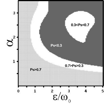
Figure 1: Probability of finding the searched state at the optimal time as function of the field parameters $\alpha,\,\varepsilon$.

4 Repeated measurements

The search algorithm we are studying makes a transition from the initial to essentially the sought state, other states being negligibly populated. Thus, any measurement process will leave the system, with high probability, in one of these two states. The probability distributions associated to the searched state $|s\rangle$, and the initial state $|j\rangle$, initially evolve according to the map of eq.(2). If at time $t_{1}$ the state is measured, the probabilities that the wavefunction collapses into either $|s\rangle$ or $|j\rangle$ are given by

$$P_{s}(t_{1}) \simeq\sin^{2}(\Omega\ t_{1})\ ,$$

$$P_{j}(t_{1}) \simeq\cos^{2}(\Omega\ t_{1})\ ,$$ (13)

respectively. If after this first measurement the system is in state $|j\rangle$ ($|s\rangle$), the probability distributions of the states $|s\rangle$ and $|j\rangle$ after a second measurement, at a time $\Delta t_{1}$ after $t_{1}$, are the eqs.(13), (the eqs.(13) exchanging $s$ and $j$), calculated at $\Delta t_{1}$. Between consecutive measurements, the system undergoes an unitary evolution. Therefore, for arbitrary intervals $\Delta t_{i}$ between consecutive measurements, the probability distributions of the states $|s\rangle$ and $|j\rangle$ at a time $t_{i+1}=t_{i}+\Delta t_{i}$ satisfy, always within the approximation $\omega_{nm}\gg\Omega$, the matrix equations

$$\binom{P_{s}(t_{i+1})}{P_{j}(t_{i+1})}=\left[\begin{array}[c]{cc}p_{i}&q_{i}\\ q_{i}&p_{i}\end{array}\right]\binom{P_{s}(t_{i})}{P_{j}(t_{i})},$$ (14)

where $p_{i}=\cos^{2}(\Omega\Delta t_{i})$ and $q_{i}=1-p_{i}$. This equation is not a Markovian process because the transition probabilities are time-interval dependent.

The general solution of the previous matrix equation for any time sequence of measurements is

$$\binom{P_{s}(t_{m})}{P_{j}(t_{m})}=\left[\begin{array}[c]{cc}\alpha_{m}&\beta_{m}\\ \beta_{m}&\alpha_{m}\end{array}\right]\binom{P_{s}(0)}{P_{j}(0)},$$ (15)

where $P_{s}(0)=0,P_{j}(0)=1$ and

$$\alpha_{m} =\frac{1}{2}\left\{1+\prod\limits_{i=0}^{m}\left[2p_{i}-1\right]\right\}$$

$$\beta_{m} =\frac{1}{2}\left\{1-\prod\limits_{i=0}^{m}\left[2p_{i}-1\right]\right\}\ .$$ (16)

If we now consider that the measurement processes are performed at regular time intervals, $t_{n}=n\Delta t$, eq. (16) becomes

$$\alpha_{m} =\frac{1}{2}\left[1+\left(\cos(2\Omega\Delta t)\right)^{m}\right]$$

$$\beta_{m} =\frac{1}{2}\left[1-\left(\cos(2\Omega\Delta t)\right)^{m}\right]\ .$$ (17)

Now, we have an unitary evolution between consecutive measurements, and the global evolution is a Markovian process, as all the $\Delta t_{i}$ are equal.

Let us now consider applications of the above eqs.(15-17). In the case where the value of the optimal time $\tau$ is only approximately known, we take a single measurement at a time equal to our estimate of $\mathbf{\tau}$, which we designate as $\mathbf{\tau}^{\mathbf{\ast}}$. In that case the probability to find the searched state after the measurement is simply given by

$$P_{s}(\mathbf{\tau}^{\mathbf{\ast}})=\frac{1}{2}\left[1-\cos(2\Omega\mathbf{\tau}^{\mathbf{\ast}})\right]\simeq 1-\frac{\pi^{2}}{4}\left(\frac{\mathbf{\tau}^{\mathbf{\ast}}-\mathbf{\tau}}{\mathbf{\tau}}\right)^{2},$$ (18)

which shows that the probability of finding the searched state, $P_{s}(\mathbf{\tau}^{\mathbf{\ast}}),$ decreases quadratically with the relative error in the estimate of the optimal time.

In Fig. 2 we present the probabilities of the searched and the initial states as a function of the number of measurements $m$, in a case where $\Delta t=\tau^{\ast}$and the relative error is$\ (\mathbf{\tau}^{\mathbf{\ast}}-\tau)/\tau=0.2$. The full and the dashed lines correspond to the previous treatment, the circles ($P_{j})$ and the stars ($P_{s}$) are the results obtained from a direct solution of the Schrödinger equation for the quantum rotor $H_{0}$, and for an ensemble of $500$ trajectories with $N=50.$ We notice that after the first measurement the value of $P_{s}$ is close to $0.9$. One also notices that after many measurements this value tends to $0.5$.

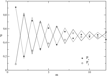
Figure 2: Probabilities of the searched ($P_{s}$) and the initial ($P_{j}$) states as a function of the number of measurements ($m$), for fixed $\Delta t=\tau^{\ast}$. The dashed and the full lines correspond to the theoretical development, eq. (17) in the same two cases, respectively.

We remark that eq.(17) implies that for a sufficiently large number of measurements, both $P_{s}$ and $P_{j}$ tend to $1/2$, independently of the interval between measurements $\Delta t$ and the initial conditions. Further inspection of Fig. 2 shows that the average value of $P_{s}$ over different number of measurements $m$ is also $1/2$. This means that the algorithm can be still useful, as it may yield the searched state with a probability $0.5,$ even in the complete absence of knowledge on the number of states on which the search is performed. However, to perform this task in a reasonably small number of measurements $m$, one has to make sure $\Delta t$ is not too small, see eq.(17).

In the case where the $m$ measurements are performed in a total time $\tau=\frac{\pi}{2\Omega}$, where the unperturbed algorithm converges to the searched state, $\Delta t=\tau/m$, so the coefficients $\alpha_{m},\beta_{m}$ become

$$\alpha_{m} =\frac{1}{2}\left[1+\left(\cos\frac{\pi}{m}\right)^{m}\right]$$

$$\beta_{m} =\frac{1}{2}\left[1-\left(\cos\frac{\pi}{m}\right)^{m}\right]\ .$$ (19)

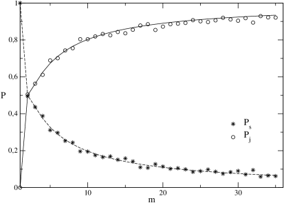
Figure 3: Probabilities of the searched ($P_{s}$) and the initial ($P_{j}$) states as a function of the number of measurements ($m$), performed in a total time $\tau$. The dashed and full lines are the theoretical results, obtained from eq.(19), in both cases, respectively.

We show in Fig. 3 the probabilities $P_{s}$ (stars), $P_{j}$ (circles) after $m$ measurements for $N=50$ and $500$ trajectories as in the previous figure. The calculation based on the direct solution of the Schrödinger equation is compared to the one obtained from eq.(19), as a function of $m$. Besides the good agreement between the two calculations we notice that $P_{s}$ decreases with $m,$ so that for $m>30$, $P_{s}<0.1$. This simply means that the more frequently the wave function collapses, the harder it becomes for the algorithm to significantly depart from the initial state. Therefore, in this case the algorithm behaves as an example of the Quantum Zeno effect, where the a high frequency of measurements hinders the departure of the system from its initial state [13, 14]. This also explains our previous assertion, that for the algorithm to be useful the time $\Delta t$ between measurements must not be too small.

5 Conclusions

We have extended the study of the search algorithm presented in [7]. There it was shown that the algorithm was robust when the energy of the searched state had some imprecision. In this work, the resonant algorithm was treated as an open system, and subject to two types of external interactions: an oscillating external field and measurement processes.

It was shown that, although the algorithm is in general affected by a periodic external field, for extensive zones of the field parameter values it works with good efficiency. In the case of measurements, the probability distribution for the searched and initial states were obtained analytically. When a set of periodic measurements are performed, the probability distribution satisfies a Master equation. In this way we have shown that the global behavior of the algorithm becomes a Markovian process. Therefore, the algorithm can still be useful in the case of repeated measurements, as long as they are not too frequent.

We believe that these results may be directly extended to the Grover algorithm. As it may be seen from the description of this algorithm in ref.[5], and as already pointed out by Grover [15], this algorithm is essentially a resonance between the searched and the average state. One should also be aware that, while in the case of the Grover algorithm care is needed to make sure that after each measurement the state of the system is reinitialized into the average state, this procedure is not required in the algorithm proposed in this work.

We acknowledge the comments made by V. Micenmacher and the support from PEDECIBA and PDT S/C/OP/28/84. R.D. acknowledges partial financial support from the Brazilian National Research Council (CNPq) and FAPERJ (Brazil). A.R and R.D. acknowledge financial support from the Brazilian Millennium Institute for Quantum Information.

References

- [1] W. Dür, R. Raussendorf, V. Kendon and H. Briegel, Phys. Rev. A 66, 052319 (2002); arXiv:quant-ph/0207137.
- [2] B. Sanders, S. Bartlett, B. Tregenna and P. Knight, Phys. Rev. A 67, 042305 (2003); arXiv:quant-ph/0207028.
- [3] J. Du, X. Xu, M. Shi, J. Wu, X. Zhou and R. Han, Phys. Rev. A 67, 042316 (2003).
- [4] G.P. Berman, D.I. Kamenev, R.B. Kassman, C. Pineda and V.I. Tsifrinovich, Int. J. Quant. Inf. 1, 51 (2003); arXiv:quant-ph/0212070
- [5] M. Nielssen and I. Chuang, Quantum Computation and Quantum Information, Cambridge University Press, 2000.
- [6] E. Farhi and S. Gutmann. Phys. Rev. A 57, 2403 (1998)
- [7] A. Romanelli, A. Auyuanet, R. Donangelo. Physica. A, (2005) also in quant-ph/
- [8] Hiroo Azuma quant-ph/0504033.
- [9] Mario Leandro Aolita and Marcos Saraceno, quant-ph/0504211
- [10] Daniel Shapira, Shay Mozes and Ofer Biham, Phys. Rev. A 67, 042301 (2003)
- [11] W. Magnus and S. Winkler, Hill´s Equation (Interscience, 1966)
- [12] I. I. Rabi, Phys. Rev 51, (1937)
- [13] B. Misra and E. C. Sudarshan, J. Math. Phys. 18, 756 (1977)
- [14] C. B. Chiu, E. C. Sudarshan and B. Misra, Phys. Rev. D 16, 520 (1977)
- [15] L. K. Grover, A.M. Sengupta, Phys. Rev. A 64, 032319 (2002), quant-ph/0109123.