On the entanglement concentration of three-partite states

Abstract

We investigate the concentration of multi-party entanglement by focusing on simple family of three-partite pure states, superpositions of Greenberger-Horne-Zeilinger states and singlets. Despite the simplicity of the states, we show that they cannot be reversibly concentrated by the standard entanglement concentration procedure, to which they seem ideally suited. Our results cast doubt on the idea that for each N there might be a finite set of N-party states into which any pure state can be reversibly transformed. We further relate our results to the concept of locking of entanglement of formation.

I Introduction

Entanglement of bi-partite states is very well studied and for pure states, the situation is particularly simple entconc : all bi-partite pure states are equivalent to singlets, as far as their entanglement is concerned, in sense that $n$ copies of the state are reversibly converted into singlets using Local Operations and Classical Communication (LOCC) in the (asymptotic) limit $n\rightarrow\infty$.

Multi-partite entanglement is much less well understood. It is known that a general multi-partite non-maximally entangled state cannot be reversibly concentrated into a collection of singlets between pairs of parties LPSW ; multiparty . It was conjectured, however, that in the asymptotic limit every pure multi-partite entangled state can be reversibly converted into combination of states from a certain Minimal Reversible Entanglement Generating Set (MREGS), which plays the role of a singlet state in a bi-partite case multiparty .

In this paper we address the question of whether the MREGS conjecture really works. We consider perhaps the simplest non-trivial case - a special kind of non-maximally entangled three-partite state that was first considered by D. Rohrlich dr :

$$|R_{p}\rangle=\sqrt{1-p} |0\rangle_{A}\frac{|0\rangle_{B}|0\rangle_{C}+|1\rangle_{B}|1\rangle_{C}}{\sqrt{2}}~{}$$

$$+\sqrt{p} |1\rangle_{A}\frac{|0\rangle_{B}|0\rangle_{C}-|1\rangle_{B}|1\rangle_{C}}{\sqrt{2}}.$$ (1)

The state was analysed in more detail in LPSW ; in particular, its asymptotic convertibility was discussed leading to the open question addressed in this paper. It is natural to conjecture that $n$ copies of $|R_{p}\rangle$ can be reversibly concentrated into collection of $nH(p)$ GHZ-states GHZ and $n[1-H(p)]$ singlets held between $B$ and $C$ in the asymptotic limit $n\rightarrow\infty$, where $H(p)=-p\log_{2}p-(1-p)\log_{2}(1-p)$ is the (Shannon) entropy of the probability distribution $\{p,1-p\}$. In LPSW evidence for this conjecture was given based on the conservation of various quantities in reversible procedures. It will also be seen below that this proportion of GHZ’s and singlets would result from the standard method of entanglement concentration.

svw contains interesting results for a number of related questions, for example the optimal rate of extraction of GHZ-states for $|R_{p}\rangle$ when the number of singlets extracted is not important.

II The standard concentration method applied to multi-party states.

The (standard) quantum entanglement concentration scheme entconc is inspired by the idea of classical Shannon compression: for example, the concentration of a large number $n$ of non-maximally entangled bi-partite states

$$|\phi_{p}\rangle^{\otimes n}=[\sqrt{1-p}|0\rangle_{A}|0\rangle_{B}+\sqrt{p}|1\rangle_{A}|1\rangle_{B}]^{\otimes n}$$ (2)

to a smaller number of maximally entangled states

$$|\phi_{\frac{1}{2}}\rangle^{\otimes k}=[\frac{1}{\sqrt{2}}(|0\rangle_{A}|0\rangle_{B}+|1\rangle_{A}|1\rangle_{B})]^{\otimes k}$$ (3)

is based on the observation, that the total initial state of $2n$ qubits, when expanded in local bases, contains typical terms of the type

$$|0^{\otimes(n-k)}1^{\otimes k}\rangle_{A}|0^{\otimes(n-k)}1^{\otimes k}\rangle_{B},$$ (4)

where $k$ has a value in the interval $[np\pm O(\sqrt{n})]$. Here $0^{\otimes(n-k)}1^{\otimes k}$ denotes some particular configuration of $k$ one’s and $n-k$ zero’s. If the measurement of a total number of $1$’s on one of the sides is performed than the result will most probably yield $k$ $1$’s, where $k\in[np\pm O(\sqrt{n})]$. In this case the initial non-maximally entangled state of $2n$ qubits will be projected to a maximally entangled state, which contains ${n\choose k}$ orthogonal terms of the type (4). Thus, the state which results if $k$ $1$’s is found is

$$\frac{1}{\sqrt{{n\choose k}}}\sum_{i=1}^{{n\choose k}}|P_{i}(0^{\otimes(n-k)}1^{\otimes k})\rangle_{A}|P_{i}(0^{\otimes(n-k)}1^{\otimes k})\rangle_{B},$$ (5)

where the sum runs over all possible permutations $P_{i}$ of $k$ one’s and $n-k$ zero’s. For large $n$ the value of ${n\choose k}$ is approximated very well by $2^{nH(p)}$ . In what follows we will often omit the argument $p$ of the entropy $H(p)$ and will denote it just by $H$.

In other words, by neglecting atypical terms, which appear with very small probability, we have got a maximally entangled state with Schmidt number $2^{nH}$.

This is, however, only part of the story, because the resulting state is now an entangled state of all $2n$ particles which is not partitioned into direct product of 2-particle maximally entangled states. This is because the state (5) “lives” in a $2^{n}\otimes 2^{n}$-dimensional Hilbert space, which is spanned by $2^{n}$ orthogonal states of $n$ qubits on each side. However, (5) contains only $2^{nH}$ orthogonal terms in Schmidt decomposition and, in principle, can be “compressed” to a $2^{nH}\otimes 2^{nH}$-dimensional Hilbert space. Thus, $n(1-H)$ qubits on each side are redundant.

To make this explicit Alice and Bob each apply a collective local unitary transformation

$$U|P_{1}(0^{\otimes(n-k)}1^{\otimes k})\rangle~{}~{}~{}~{}=|00...000\rangle|0\rangle^{\otimes n(1-H)}$$

$$U|P_{2}(0^{\otimes(n-k)}1^{\otimes k})\rangle~{}~{}~{}~{}=|00...001\rangle|0\rangle^{\otimes n(1-H)}$$

$$U|P_{3}(0^{\otimes(n-k)}1^{\otimes k})\rangle~{}~{}~{}~{}=|00...010\rangle|0\rangle^{\otimes n(1-H)}$$ (6)

$$.~{}~{}~{}~{}~{}~{}.~{}~{}~{}~{}~{}~{}.~{}~{}~{}~{}~{}~{}.~{}~{}~{}~{}~{}~{}.~{}~{}~{}~{}~{}~{}.~{}~{}~{}~{}~{}~{}.$$

$$U|P_{2^{nH}}(0^{\otimes(n-k)}1^{\otimes k})\rangle~{}=|11...111\rangle|0\rangle^{\otimes n(1-H)}$$

on their particles, which re-arranges this state to a $2^{nH}\otimes 2^{nH}$-dimensional subspace of the original Hilbert space and sets all redundant qubits to some standard state, e.g. the all $|0\rangle$-state. This local transformation is isomorphic to classical Shannon compression where $2^{nH}$ typical sequences which have a length $n$ are relabelled using $2^{nH}$ codewords which have length $nH$. It is easy to check that the new state of $2nH$ qubits is nothing but the direct product of $nH$ separate EPR-states, i.e. (3). Thus, as a result of (II) the total state (5) of $2n$ particles is converted to

$$\biggl{[}\frac{1}{\sqrt{2}}(|0\rangle_{A}|0\rangle_{B}+|1\rangle_{A}|1\rangle_{B})\biggr{]}^{\otimes nH}\otimes\biggl{[}|0\rangle_{A}|0\rangle_{B}\biggr{]}^{\otimes n(1-H)}.$$ (7)

Consider now the following three-particle bi-partite state

$$|\Phi_{p}\rangle^{\otimes n}=(\sqrt{p}|0\rangle_{A}|{\theta}\rangle_{B_{1}B_{2}}+\sqrt{1-p}|1\rangle_{A}|{\tau}\rangle_{B_{1}B_{2}})^{\otimes n}.$$ (8)

Here $|{\theta}\rangle_{B_{1}B_{2}}$, $|{\tau}\rangle_{B_{1}B_{2}}$ are normalised orthogonal but otherwise general states of two particles $B_{1}$ and $B_{2}$ located on Bob’s side. The entanglement concentration procedure will work in this case just as before, since Bob is able to apply all operations described above working locally with the states $|{\theta}\rangle_{B_{1}B_{2}}$, $|{\tau}\rangle_{B_{1}B_{2}}$ of two particles exactly as he would work with the states $|0\rangle_{B}$, $|1\rangle_{B}$ of one particle (see Fig. 1, (ii)). As a result, Alice and Bob will be able reversibly to concentrate $n$ copies of (8) into $nH$ copies of the maximally entangled state

$$|\Phi_{\frac{1}{2}}\rangle=\frac{1}{\sqrt{2}}(|0\rangle_{A}|{\theta}\rangle_{B_{1}B_{2}}+|1\rangle_{A}|{\tau}\rangle_{B_{1}B_{2}}),$$ (9)

while the other $n(1-H)$ initially non-maximally entangled “triples” are now in the state $|0\rangle_{A}|{\theta}\rangle_{B_{1}B_{2}}$. Thus the total state is

$$\biggl{[}\frac{1}{\sqrt{2}}(|0\rangle_{A}|{\theta}\rangle_{B_{1}B_{2}}+|1\rangle_{A}|{\tau}\rangle_{B_{1}B_{2}})\biggr{]}^{\otimes nH}~{}~{}~{}~{}~{}~{}~{}~{}~{}$$ (10)

$$~{}~{}~{}~{}~{}~{}~{}~{}~{}~{}~{}~{}~{}~{}~{}~{}~{}~{}~{}\otimes\biggl{[}|0\rangle_{A}|{\theta}\rangle_{B_{1}B_{2}}\biggr{]}^{\otimes n(1-H)}.$$

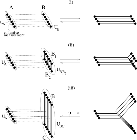
Figure 1: (i): Standard bi-partite entanglement concentration scheme. Alice performs collective measurement on her side followed by local unitary transformations $U_{A}$ and $U_{B}$. The process is reversible in the asymptotic limit. (ii): The scheme works similarly in the case when there are two particles (for each state) on Bob’s side. Bob performs the local unitary transformation $U_{B_{1}B_{2}}$ on $2n$ qubits on his side. The process is reversible in the asymptotic limit. (iii): $2n$ qubits initially held by Bob are distributed now between Bob and Claire. The question is whether Bob and Claire can perform $U_{BC}$ using LOCC only.

Now suppose that initially Bob gives one of his particles to Claire:

$$|\Psi_{p}\rangle^{\otimes n}=(\sqrt{p}|0\rangle_{A}|{\theta}\rangle_{BC}+\sqrt{1-p}|1\rangle_{A}|{\tau}\rangle_{BC})^{\otimes n}$$ (11)

Starting the procedure in the same way as we did in the case of (8) we will soon get the following analog of (5):

$$\frac{1}{\sqrt{2^{nH}}}\sum_{i}|P_{i}(0^{\otimes(n-k)}1^{\otimes k})\rangle_{A}|P_{i}({\theta}^{\otimes(n-k)}{\tau}^{\otimes k})\rangle_{BC},$$ (12)

where the sum runs over all possible permutations $P_{i}$. From the point of view of $A$ the procedure continues from here in the same way, namely Alice can apply local transformation (II) on her local qubits. However, $B$ and $C$ must jointly apply a bi-partite analog $U_{BC}$ of (II) on their qubits. This transformation may be written simply by replacing $|0\rangle$, $|1\rangle$ with $|{\theta}\rangle$, $|{\tau}\rangle$ in (II):

$$|P_{1}({\theta}^{\otimes(n-k)}{\tau}^{\otimes k})\rangle~{}~{}~{}~{}\rightarrow|{\theta}{\theta}...{\theta}{\theta}{\theta}\rangle|{\theta}^{\otimes n(1-H)}\rangle$$

$$|P_{2}({\theta}^{\otimes(n-k)}{\tau}^{\otimes k})\rangle~{}~{}~{}~{}\rightarrow|{\theta}{\theta}...{\theta}{\theta}{\tau}\rangle|{\theta}^{\otimes n(1-H)}\rangle$$

$$|P_{3}({\theta}^{\otimes(n-k)}{\tau}^{\otimes k})\rangle~{}~{}~{}~{}\rightarrow|{\theta}{\theta}...{\theta}{\tau}{\theta}\rangle|{\theta}^{\otimes n(1-H)}\rangle$$ (13)

$$.~{}~{}~{}~{}~{}~{}.~{}~{}~{}~{}~{}~{}.~{}~{}~{}~{}~{}~{}.~{}~{}~{}~{}~{}~{}.~{}~{}~{}~{}~{}~{}.~{}~{}~{}~{}~{}~{}.$$

$$|P_{2^{nH}}({\theta}^{\otimes(n-k)}{\tau}^{\otimes k})\rangle\rightarrow|{\tau}{\tau}...{\tau}{\tau}{\tau}\rangle|{\theta}^{\otimes n(1-H)}\rangle$$

As a side effect of this transformation, $2^{n(1-H)}$ redundant pairs of $B$ and $C$ will be in the state $|{\theta}\rangle$. Thus, if $U_{BC}$, (II), can be performed then we should get:

$$\biggl{[}\frac{1}{\sqrt{2}}(|0\rangle_{A}|{\theta}\rangle_{BC}+|1\rangle_{A}|{\tau}\rangle_{BC})\biggr{]}^{\otimes nH}\otimes\biggl{[}|0\rangle_{A}|{\theta}\rangle_{BC}\biggr{]}^{\otimes n(1-H)}.$$ (14)

The main question is whether $U_{BC}$ can be achieved by LOCC. Even if not, it might be achievable using an amount of entanglement per copy which goes to zero as $n\rightarrow\infty$. In this latter case we may use some singlets, but a number which is negligible in the asymptotic limit, and thus the transformation is still reversible. Thus, we ask what is the minimal amount of entanglement between $B$ and $C$ needed to implement $U_{BC}$ using this entanglement and LOCC.

Example I: As a first example let us consider the case when
$\displaystyle|{\theta}\rangle_{BC}$ $\displaystyle=$ $\displaystyle|0\rangle_{B}|0\rangle_{C}~{}$ $\displaystyle|{\tau}\rangle_{BC}$ $\displaystyle=$ $\displaystyle|1\rangle_{B}|1\rangle_{C}$
In this case (11) will correspond to non-maximally entangled GHZ-states:

$$|\Theta_{p}\rangle^{\otimes n}=(\sqrt{1-p}|0\rangle_{A}|0\rangle_{B}|0\rangle_{C}+\sqrt{p}|1\rangle_{A}|1\rangle_{B}|1\rangle_{C})^{\otimes n}$$ (16)

If $U_{BC}$ can be performed then we should get $nH$ copies of GHZ-state
$\displaystyle\frac{1}{\sqrt{2}}(|0\rangle_{A}|{\theta}\rangle_{BC}+|1\rangle_{A}|{\tau}\rangle_{BC})~{}~{}~{}~{}~{}~{}~{}~{}~{}~{}~{}$ $\displaystyle=\frac{1}{\sqrt{2}}(|0\rangle_{A}|0\rangle_{B}|0\rangle_{C}+|1\rangle_{A}|1\rangle_{B}|1\rangle_{C})$
and $n(1-H)$ copies of $|0\rangle_{A}|{\theta}\rangle_{BC}=|0\rangle_{A}|0\rangle_{B}|0\rangle_{C}$:

$$\biggl{[}\frac{1}{\sqrt{2}}(|0\rangle_{A}|0\rangle_{B}|0\rangle_{C}+|1\rangle_{A}|1\rangle_{B}|1\rangle_{C})\biggr{]}^{\otimes nH}~{}~{}~{}~{}~{}~{}~{}~{}~{}$$ (18)

$$~{}~{}~{}~{}~{}~{}~{}~{}~{}~{}~{}~{}~{}~{}~{}~{}~{}~{}~{}\otimes\biggl{[}|0\rangle_{A}|0\rangle_{B}|0\rangle_{C}\biggr{]}^{\otimes n(1-H)}.$$

Clearly there is a possible bi-partite unitary $U_{BC}$ of the form $U_{B}\otimes U_{C}$ ($U_{B}$ and $U_{C}$ being of the form (II)) which may be implemented locally by Bob and Claire. Thus, $n$ non-maximally entangled GHZ-states can be reversibly concentrated to $nH$ maximally entangled GHZ-states plus $n(1-H)$ direct products.

Example II: We now arrive at the main point. We consider the following choices of bi-partite states (introduced in dr )
$\displaystyle|{\theta}\rangle_{BC}=\frac{1}{\sqrt{2}}(|0\rangle_{B}|0\rangle_{C}+|1\rangle_{B}|1\rangle_{C})~{}$ $\displaystyle|{\tau}\rangle_{BC}=\frac{1}{\sqrt{2}}(|0\rangle_{B}|0\rangle_{C}-|1\rangle_{B}|1\rangle_{C}).$

This leads to what we call the Rohrlich state (I), which now can be rewritten in terms of $|{\theta}\rangle$ and $|{\tau}\rangle$ as

$$|R_{p}\rangle=\sqrt{1-p}|0\rangle_{A}|{\theta}\rangle_{BC}+\sqrt{p}|1\rangle_{A}|{\tau}\rangle_{BC}$$ (20)

We note that the state $|R_{1\over 2}\rangle$ is locally equivalent to a GHZ state, and the state $|R_{0}\rangle$ comprises a singlet held between Bob and Claire.

If $U_{BC}$ could be implemented locally in this case then $n$ copies of $|R_{p}\rangle$ would be reversibly converted (in the asymptotic limit) into $nH$ GHZ states and $n(1-H)$ singlets between Bob and Claire:

$$\biggl{[}\frac{1}{\sqrt{2}}(\frac{|0\rangle_{A}+|1\rangle_{A}}{\sqrt{2}~{}~{}}|0\rangle_{B}|0\rangle_{C}+\frac{|0\rangle_{A}-|1\rangle_{A}}{\sqrt{2}~{}~{}}|1\rangle_{B}|1\rangle_{C})\biggr{]}^{\otimes nH}$$

$$\otimes\biggl{[}|0\rangle_{A}\frac{1}{\sqrt{2}}(|0\rangle_{B}|0\rangle_{C}+|1\rangle_{B}|1\rangle_{C})\biggr{]}^{\otimes n(1-H)};~{}~{}~{}~{}~{}~{}~{}$$ (21)

which is consistent with the conjecture in LPSW .

In this paper we show that using the standard concentration procedure such a transformation is impossible. Our conclusion follows from examination of the amount of non-locality in $U_{BC}$: we find that it is not negligible, but proportional to $n$ as $n\rightarrow\infty$.

Here we use the following method in order to find the amount of non-locality in $U_{BC}$ (see also Toffoli ). We act with $U_{BC}$ on a test state $|\Psi_{in}^{test}\rangle_{BC}$:

$$U_{BC}|\Psi_{in}^{test}\rangle=|\Psi_{out}^{test}\rangle,$$ (22)

where the test state is a superposition of basic input states in (II). We denote the amount of non-locality between $B$ and $C$ possessed by $|\Psi_{in}^{test}\rangle_{BC}$ and $|\Psi_{out}^{test}\rangle_{BC}$ by $E_{in}^{test}$ and $E_{out}^{test}$ respectively, where $E=S(Tr_{B}|\Psi\rangle\langle\Psi|)=S(Tr_{C}|\Psi\rangle\langle\Psi|)$ is the von Neumann entropy of the reduced density matrix. If $|\Psi_{in}^{test}\rangle_{BC}$, $|\Psi_{out}^{test}\rangle_{BC}$ possess different amount of entanglement, then $U_{BC}$ is non-local. The amount of non-locality in $U_{BC}$ is not less than the entanglement difference between the two states: $E_{U}\geq|E_{in}^{test}-E_{out}^{test}|$ (acting on different test states $U_{BC}$ may produce different amounts of entanglement).

III An example: $n$=4.

It turns out that in the non-asymptotic case of $n=2$ this transformation can be implemented by LOCC. Indeed,

$$|{\theta}\rangle|{\tau}\rangle\rightarrow|{\theta}\rangle|{\theta}\rangle$$

$$|{\tau}\rangle|{\theta}\rangle\rightarrow|{\tau}\rangle|{\theta}\rangle$$

is nothing but a partial CNOT transformation on logical bits encoded nonlocally in the states $|{\theta}\rangle$, $|{\tau}\rangle$ followed by a NOT on the second logical qubit. It can be easily checked explicitly that this nonlocal CNOT transformation can be built from local CNOT gates.

However, for $n>2$ this transformation cannot be implemented by LOCC Toffoli . Let us illustrate this for $n=4$. Consider the case of a single $|{\tau}\rangle$. Here two qubits are redundant on each side and $U_{BC}$ maps the four possible terms as follows

$$U_{BC}|{\theta}{\theta}{\theta}{\tau}\rangle=|{\theta}{\theta}{\theta}{\theta}\rangle~{}$$

$$U_{BC}|{\theta}{\theta}{\tau}{\theta}\rangle=|{\theta}{\tau}{\theta}{\theta}\rangle~{}$$ (23)

$$U_{BC}|{\theta}{\tau}{\theta}{\theta}\rangle=|{\tau}{\theta}{\theta}{\theta}\rangle~{}$$

$$U_{BC}|{\tau}{\theta}{\theta}{\theta}\rangle=|{\tau}{\tau}{\theta}{\theta}\rangle,$$

i.e. two last pairs are in the $|{\theta}\rangle$-state while two first pairs carry the information about the four possible inputs.

It is useful to consider the action of $U_{BC}$, defined in (III), on a superposition. In particular, $U_{BC}$ will transform the following test state

$$|\Psi_{in}^{test}\rangle_{BC}={1\over 2}\biggl{(}|{\theta}{\theta}{\theta}{\tau}\rangle_{BC}+|{\theta}{\theta}{\tau}{\theta}\rangle_{BC}~{}~{}~{}~{}~{}~{}~{}$$

$$+|{\theta}{\tau}{\theta}{\theta}\rangle_{BC}+|{\tau}{\theta}{\bf}{\theta}{\theta}\rangle_{BC}\biggr{)}$$ (24)

to the state

$$|\Psi_{out}^{test}\rangle_{BC}={1\over{2}}\biggl{(}|{\theta}{\theta}\rangle_{BC}+|{\theta}{\tau}\rangle_{BC}~{}~{}~{}~{}~{}~{}~{}~{}~{}~{}~{}~{}~{}~{}~{}~{}~{}~{}~{}~{}~{}~{}~{}~{}~{}~{}~{}~{}~{}$$

$$+|{\tau}{\theta}\rangle_{BC}+|{\tau}{\tau}\rangle_{BC}\biggr{)}|{\theta}{\theta}\rangle_{BC}~{}~{}~{}~{}~{}~{}~{}~{}~{}~{}$$ (25)

$$~{}~{}~{}~{}~{}~{}~{}~{}~{}~{}~{}~{}~{}~{}=(|{\theta}\rangle_{BC}+|{\tau}\rangle_{BC})(|{\theta}\rangle_{BC}+|{\tau}\rangle_{BC})|{\theta}{\theta}\rangle_{BC}.$$

If $U_{BC}$ could be implemented by a local transformation (i.e., if $U_{BC}=U_{B}\otimes U_{C}$) then the entanglement $E_{in}^{test}$ must equal $E_{out}^{test}$. We now show that this is not the case.

$E_{in}^{test}$ may be calculating by noting that the computational basis for Bob and Claire is a Schmidt basis. For any binary string $b\in\{0,1\}^{4}$, the term $|b\rangle_{B}|b\rangle_{C}$ occurs in the superposition (III) with an amplitude which depends only on the number, $i$, of $1$’s in the binary string $b$. Let us call the amplitude of a term with $i$ $1$’s, $\xi_{i}$. Then $(\xi_{0},\xi_{1},\xi_{2},\xi_{3},\xi_{4})=({1\over 2},{1\over 4},0,-{1\over 4},-{1\over 2})$, thus the entanglement $E_{in}^{test}=-\sum_{i=0}^{4}{4\choose i}\xi_{i}^{2}\log_{2}(\xi_{i}^{2})=3~{}ebits$. The final state $|\Psi_{out}^{test}\rangle_{BC}$ clearly has $E_{out}^{test}=2~{}ebits$. We note, for future use, the the four terms $|{\theta}{\theta}\rangle_{BC}$, $|{\theta}{\tau}\rangle_{BC}$, $|{\tau}{\theta}\rangle_{BC}$, and $|{\tau}{\tau}\rangle_{BC}$ that emerge from the compression add up in such a way that their superposition is not entangled being a product of two copies of $(|{\theta}\rangle_{BC}+|{\tau}\rangle_{BC})$, each of them being unentangled. The only entanglement comes from the “factored out” states $|{\theta}{\theta}\rangle_{BC}$. Thus we conclude that no unitary $U_{BC}$ which acts as (III) can be of the form $U_{B}\otimes U_{C}$.

Since $|\Psi_{out}^{test}\rangle_{BC}$, $|\Psi_{in}^{test}\rangle_{BC}$ possess different amounts of entanglement, we cannot claim that in general reversible entanglement concentration is possible. It might be the case, however, that in the asymptotic limit the ratio $|E_{in}-E_{out}|/E_{in}$ goes to zero. Thus, our next step is to find out how $|E_{in}-E_{out}|$ grows with $n$.

IV Calculation of the entanglement difference for general $n$.

We have used a combination of analytical and numerical techniques to find the $|E_{in}-E_{out}|$ vs. $n$ dependance.

First we derive the formula for the entanglement possessed by $|\Psi_{in}^{test}\rangle_{BC}$ as a function of $n$ for the given ratio $p=k/n$, where $k$ is the number of ${\tau}$’s. As the generalization of (III), we consider the following test state:

$$|\Psi_{in}^{test}\rangle_{BC}=\frac{1}{\sqrt{{n\choose np}}}\sum_{j}^{n\choose np}|P_{j}({\theta}^{\otimes(n-k)}{\tau}^{\otimes k})\rangle_{BC}.$$ (26)

where the sum runs over all possible permutations $P_{j}$ of $k$ $\tau$’s and $n-k$ $\theta$’s in $n$ places.

As in the case of $n=4$ the computational basis for Bob and Claire is a Schmidt basis and for any binary string $b\in\{0,1\}^{n}$, the term $|b\rangle_{B}|b\rangle_{C}$ occurs in the superposition (26) with an amplitude which depends only on the number, $i$, of $1$’s in the binary string $b$. Let us denote, as before, the amplitude with $i$ $1$’s, $\xi_{i}$. Then the entanglement is

$$E_{in}^{test}=-\sum_{i=0}^{n}{n\choose i}\xi_{i}^{2}\log_{2}(\xi_{i}^{2}),$$ (27)

where

$$\xi_{i}=\frac{1}{\sqrt{2^{n}{n\choose np}}}\sum_{x=\max(0,i-(1-p)n)}^{\min(i,np)}(-1)^{x}{n-i\choose np-x}{i\choose x}.$$ (28)

The entanglement $E_{out}^{test}$ is straightforward to compute in the case that ${n\choose k}$ is an integer power of $2$. ${n\choose k}=2^{N_{exact}}$, say. In this case, as in Eq. (III), $|\Psi_{out}^{test}\rangle_{BC}$ is (up to normalisation) a product of two terms; the first term is a product of $N_{exact}$ copies of ($|\theta\rangle+|\tau\rangle$) and the second is a product of $n-N_{exact}$ copies of $|\theta\rangle$. Thus, since $|\theta\rangle+|\tau\rangle$ is unentangled, the entanglement is

$$E_{out}^{test} = n-N_{exact}=n-\log_{2}{n\choose k}$$ (29)

$$\sim n-\log_{2}{n\choose np}\sim n[1-H(p)].$$

The case when ${n\choose k}$ is not an integer power of $2$ is more involved to analyse. However a similar situation arises in the standard bi-partite situation entconc . One has $n$ copies of $\sqrt{1-p}|0\rangle_{A}|0\rangle_{B}+\sqrt{p}|1\rangle_{A}|1\rangle_{B}$ and Alice projects onto a state with a given number, $k$, of $1$’s. In this case the issue is that Alice’s projection typically results in a state with a Schmidt number which is not an integer power of $2$. Thus one cannot immediately interpret the state as a certain number of singlets held between Alice and Bob. However, as shown in entconc , by taking batches of $n$ copies of the state ($M$ batches, say), one can always arrange things so that the total state of the $M$ batches is as close as we like to a state with a Schmidt number an integer power of $2$. A similar argument can be made in our situation. Details are given in the Appendix. The result is that, just as in the case where ${n\choose k}$ is an integer power of $2$, $E_{out}^{test}\sim n[1-H(p)]$ with high probability.

Using these expressions we have calculated $E_{in}^{test}$ and $E_{out}^{test}$ for different values of $p$ and $n$. Fig. 2 gives numerical results for $E_{in}^{test}$, $E_{out}^{test}$ as a function of $n$ for $p=0.8$. A linear dependance $|E_{in}^{test}-E_{out}^{test}|\cong 0.466n$ is obtained. Our calculations showed a similar behaviour for other values of $p$. The calculated slopes $|E_{in}^{test}-E_{out}^{test}|/n$ for several values of $p$ are plotted in Fig. 3. We conclude, therefore, that since the ratio $|E_{in}^{test}-E_{out}^{test}|/E_{in}^{test}$ is constant for given $p$, the entanglement concentration of $|R_{p}\rangle$-states cannot be performed reversibly using this standard protocol even in the asymptotic limit.

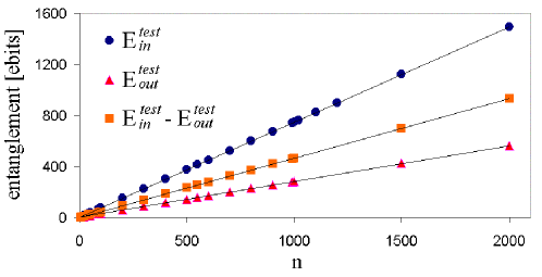
Figure 2: Entanglement as a function of the number of copies, $n$, for $p=0.8$. $E_{in}^{test}$ is computed numerically from (27) and (28); the values of $n$ were chosen so that $np$ was an integer. For $E_{out}^{test}$ we have plotted $n-\log_{2}{n\choose np}$. (The validity of this approximation is discussed in detail in the text.)

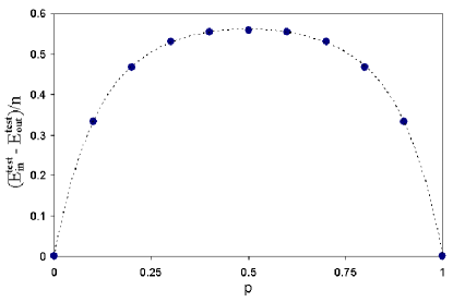
Figure 3: Numerical results for $|E_{in}^{test}-E_{out}^{test}|/n$ as a function of $p$.

V Locking of entanglement of formation and the question of (im)possibility of reversible concentration.

LPSW provides us with necessary criteria for existence of a reversible transformation of multi-partite entanglement: the entropy of entanglement for all bi-partite partitions and the relative entropy of entanglement for any two parties must remain constant. In particular, for a three-partite state, six quantities must be conserved: von Neumann entropies of three reduced density matrices $S(\rho_{A})$, $S(\rho_{B})$ and $S(\rho_{C})$, and relative entropies of three bi-partite reduced density matrices $E_{re}(\rho_{AB})$, $E_{re}(\rho_{BC})$ and $E_{re}(\rho_{AC})$.

The bi-partite entanglement $E_{A(BC)}=S(\rho_{A})=nH(p)$ and $E_{B(AC)}=E_{C(AB)}=S(\rho_{B})=n$ possessed by the state (II) is equal to the entanglement possessed by $n$ copies of the initial state (20). Indeed, the fact that this hypothetical reversible concentration procedure is consistent with these constraints, as noted in LPSW , was a main motivation for this paper.

We note, however, that another measure of entanglement, the entanglement of formation $E_{F}$ wootters , would not be conserved in this hypothetical reversible transformation. Indeed, in our case $E_{F}$ can be easily calculated using definitions and results of wootters , and for the initial state $E_{F}(\rho_{BC}^{in})=nH({1\over 2}+\sqrt{p(1-p)})$, while for the final state $E_{F}(\rho_{BC}^{out})=n(1-H(p))$. Here we used the result from E_F_additivity that $E_{F}$ of mixtures of the Bell-states is additive. In general, the question of additivity of the entanglement of formation is still open.

Although, $E_{F}$ is not conserved in our hypothetical transformation, this does not automatically rule out the transformation. Indeed the entanglement of formation $E_{F}(\rho_{BC})$ can be increased by assistance from Alice. However, an important question is how much must Alice pay (in destroying her state) in order to increase $E_{F}(\rho_{BC})$. One is tempted to assume that $|\Delta S(\rho_{A})|\geq|\Delta E_{F}(\rho_{BC})|$, i.e. that if Alice gains one bit of information from her system (by measurement), then she cannot help Bob and Claire increase their $E_{F}$ by more than 1 e-bit. If this were the case it then follows that $|R_{p}\rangle$ cannot be reversibly concentrated to GHZ’s and EPR’s by any method, because Alice would need to destroy her entanglement with $BC$ by $n[H({1\over 2}+\sqrt{p(1-p)})+H(p)-1]$.

On the other hand, very recently, the effect of locking of entanglement of formation locking was discovered. For some states $\rho_{BC}$ the entanglement of formation $E_{F}(\rho_{BC})$ can be increased by much more than the information received from Alice. In principle, a single bit from Alice can result in an increase of $E_{F}(\rho_{BC})$ by an arbitrarily large amount. This offers the possibility that in our case Alice need not destroy her entanglement with $BC$ but still allow for the required increase in $E_{F}(\rho_{BC})$, and hence it might be possible to have reversible transformation of $|R_{p}\rangle$-states into GHZ’s and EPR’s.

We note however, that if the latter scenario were true, this would be an example of locking of $E_{F}$ very different from the original example analysed in locking . The example in locking is of a specially constructed state, while in our case the state is simply a product of GHZ’s and EPR’s. Furthermore, we are considering an asymptotic situation (blocks of states) while the example of locking is for a single state.

VI Discussion

In the present paper we analyzed only one particular method, the “the standard method”, for concentrating entanglement in the case of Rohrlich states. Using this procedure, reversible concentration of $|R_{p}\rangle$ into GHZ’s and singlets is not possible. What can we conclude from this?

$\bullet$ First of all, although the state $|R_{p}\rangle$ was chosen precisely because it seemed suited to concentration via the standard protocol and it is hard to believe that other methods could do better, that is still an open possibility. In this context we make a number of observations:

a) We note, that in bi-partite case the task is essentially symmetric under interchange of the roles that two parties play in the protocol. This is not the case for three-partite interpolating states (20). If the parties interchange their roles then two schemes might appear as essentially different. The standard method that we consider here is of a “$A\rightarrow(BC)$” type, i.e. Alice performs a collective local measurement on her side, then reports the result to Bob and Claire, which are required to complete the protocol by collective local unitaries on their sides. Other methods, e.g. “$B\rightarrow(AC)$” type, are beyond the scope of this article.

Is the “$A\rightarrow(BC)$” method presented here optimal amongst all possible $A\rightarrow(BC)$ schemes? Optimality of the standard method in bi-partite case follows from its reversibility. Since the same method becomes irreversible when applied to three-partite interpolating state, we cannot use the same argument to show its optimality. Can we claim that the standard method we use here is the most general method one can use? (If it is, then its optimality will follow.) In the most general terms, the task is to transform $|R_{p}\rangle^{\otimes n}$ into (II). In the asymptotic limit $|R_{p}\rangle^{\otimes n}$ almost entirely lies in its typical subspace, i.e.

$$|R_{p}\rangle^{\otimes n}\approx|\Omega\rangle=\sum_{k=np-O(\sqrt{n})}^{np+O(\sqrt{n})}\frac{1}{\sqrt{2^{nH}}}\sum_{i}|P_{i}(0^{\otimes(n-k)}1^{\otimes k})\rangle_{A}|P_{i}({\theta}^{\otimes(n-k)}{\tau}^{\otimes k})\rangle_{BC}.$$ (30)

Alice’s local collective measurement projects $|\Omega\rangle$ into a subspace of the typical subspace, i.e. into the state (12) with a particular value of $k$. The only way to transform (12) to (II) is to “rename” the states. This is exactly what $U_{BC}$ does. Thus, $U_{BC}$ is most general operation needed to convert (12) into (II). However we have not ruled out the possibility that a different measurement done by Alice could project $|\Omega\rangle$ into a state which might be converted into (II) using a “cheaper” $\tilde{U}_{BC}$.

b) It is worth noting, that the standard method presented here has features which seem undesirable in certain regimes. For example, let us consider the situation when initially Alice, Bob and Claire share $n$ pairs (20) which are already maximally entangled, i.e. $p=0.5$. Clearly in this case they should not do anything. However if they apply the concentration protocol, then they will consume approximately $0.56n$ ebits as can be seen from Fig. 3. It is not clear, however, whether this inefficiency is an essential feature of any $|R_{p}\rangle$-state concentration protocol, or only of our method.

c) Using the standard method we required that the final state should be exactly given by singlets and GHZ’s. This task demands that Bob and Claire must use a significant amount of entanglement to implement the required $U_{BC}$ transformation. It is possible, however, that if we accept a final state that is only approximately equal to a combination of singlets and GHZ’s (where the precise details of the quality of the approximation needs to be defined appropriately), the non-locality needed by Bob and Claire becomes negligibly small.

$\bullet$ Second, it might of course be possible that the states $|R_{p}\rangle$ can be reversibly concentrated to members of three-party MREGS other than GHZ’s and singlets. This is possible despite the fact that the concentration into EPR’s and GHZ’s is so natural, both because this is what the standard method suggests as well as the entropy considerations in LPSW .

$\bullet$ Third, of course, it is also possible that that reversible concentration of $|R_{p}\rangle$ and multi-partite states in general is not possible.

VII Conclusion

We have analyzed the most natural way to concentrate multiparticle entanglement in arguably the simplest non-trivial case. We showed that the standard method does not work. This does not however settle the question. There might be other methods that work, there might be other MREGS than the one we have considered, or, of course, concentration might fail altogether. Despite the partial nature of our results, we feel that our analysis leads to a much better understanding of the structure of this problem and has implications for other areas of quantum information.

Appendix A The entanglement of the test state

In the text in Sec. IV we noted that when Alice measures her system, she will find $k$ $1$’s out of a total of $n$, but that ${n\choose k}$ may not be an integer power of $2$. The computation of $E_{out}^{test}$ is simple when ${n\choose k}$ is a power of $2$; and with high probability $k$ will be close to $np$ and therefore $E_{out}^{test}\sim n[1-H(p)]$. If ${n\choose k}$ is not an integer power of $2$ then we need to adapt the procedure in order to get direct product of perfect GHZ’s. Here we show that when we do so, the leading order behaviour is still that $E_{out}^{test}\sim n[1-H(p)]$ with high probability.

We will follow the standard bi-partite concentration procedure entconc and take $M$ batches with $n$ states in each batch. Measurement of the $i$-th batch yields $k_{i}$ one’s. Let $D_{M}$ denote the accumulated product $\Pi_{i=1}^{M}{n\choose k_{i}}$. We continue measuring batches of $n$ states until $D_{M}$ is in the interval $[2^{l},2^{l}(1+\epsilon)]$, for some integer $l$ and some small fixed $\epsilon$. The expected number of batches is $1/\epsilon$, and the expected total number of states in the ensemble is, therefore, $N=n/\epsilon$.

$U_{BC}$ acts on the complete set of batches. Each term is a string of $\log_{2}D_{M}$ qubit pairs; each qubit pair is in the state $|\theta\rangle$ or the state $|\tau\rangle$. $U_{BC}$ transforms (“compresses”) each string to one in which the trailing qubits are all in the state $|\theta\rangle$ [cf Eqn. (III)].

As in the body of the text, we will bound the entanglement in $U_{BC}$ by considering its action on a test state. We take as a test state the tensor product of the bi-partite test states used in the text, one for each batch of $n$ pairs:

$$|\Theta_{in}^{test}\rangle=|\Psi_{in}^{test}(k_{1})\rangle\otimes|\Psi_{in}^{test}(k_{2})\rangle\otimes...\otimes|\Psi_{in}^{test}(k_{M})\rangle.$$ (31)

The entanglement of $|\Theta_{in}^{test}\rangle$ is the sum of the entanglement of all states $|\Psi_{in}^{test}(k_{i})\rangle_{BC}$, which in the asymptotic limit is just $n$ times the entanglement of a single $|\Psi_{in}^{test}(k)\rangle_{BC}$ with $k=np$, which we calculated numerically in the body of the text.

$|\Theta_{out}^{test}\rangle$ is a product of two terms

$$|\Theta_{out}^{test}\rangle=|\Gamma_{M}\rangle\otimes|{\theta}{\theta}{\theta}...{\theta}\rangle,$$ (32)

where

$$|\Gamma_{M}\rangle= {1\over\sqrt{\gamma}}\biggl{[}|{\theta}\rangle\biggl{(}|{\theta}.....{\theta}{\theta}\rangle+|{\theta}.....{\theta}{\tau}\rangle+...+|{\tau}.....{\tau}{\tau}\rangle\biggr{)}$$ (33)

$$+|{\tau}\rangle\biggl{(}|{\theta}........{\theta}\rangle+...+|{\theta}{\theta}...{\theta}{\tau}...\rangle\biggr{)}\biggr{]},~{}~{}~{}~{}$$

where $\gamma$ is a normalisation factor and equals the total number of terms and lies between $2^{l}$ and $2^{l}(1+\epsilon)$, i.e. $\gamma=2^{l}(1+\epsilon^{{}^{\prime}})$, where $0\leq\epsilon^{{}^{\prime}}\leq\epsilon$. The number of $\theta$’s in the second term of (32) will be close to $Mn(1-H)=N(1-H)$ with high probability.

Thus $|\Gamma_{M}\rangle$ can be written

$$|\Gamma_{M}\rangle=\sqrt{1\over{1+\epsilon^{{}^{\prime}}}}|\phi_{1}\rangle+\sqrt{\epsilon^{{}^{\prime}}\over{1+\epsilon^{{}^{\prime}}}}|\phi_{2}\rangle,$$ (34)

where

$$|\phi_{1}\rangle={1\over\sqrt{2^{l}}}|{\theta}\rangle\biggl{(}|{\theta}.....{\theta}{\theta}\rangle+...+|{\tau}.....{\tau}{\tau}\rangle\biggr{)}$$ (35)

contains the first $2^{l}$ terms and

$$|\phi_{2}\rangle={1\over\sqrt{\epsilon^{{}^{\prime}}2^{l}}}|{\tau}\rangle\biggl{(}|{\theta}........{\theta}\rangle+...+|{\theta}{\theta}...{\theta}{\tau}...\rangle\biggr{)}$$ (36)

the remaining $\epsilon^{{}^{\prime}}2^{l}$ terms ($|\phi_{1}\rangle$ and $|\phi_{2}\rangle$ are orthogonal and normalised).

We now use the fact bound that for any two bi-partite pure orthogonal states $|\phi_{1}\rangle$ and $|\phi_{2}\rangle$, the entanglement of the superposition $\alpha|\phi_{1}\rangle+\beta|\phi_{2}\rangle$ satisfies:

$$E(\alpha|\phi_{1}\rangle+\beta|\phi_{2}\rangle)\leq 2[|\alpha|^{2}E(\phi_{1})+|\beta|^{2}E(\phi_{2})+H(|\alpha|^{2})].$$ (37)

The entanglement of $|\phi_{1}\rangle$ is 1 ebit, while the entanglement of $|\phi_{2}\rangle$ is at most $N$.

Also ${\epsilon^{{}^{\prime}}\over{1+\epsilon^{{}^{\prime}}}}\leq\epsilon$, ${1\over{1+\epsilon^{{}^{\prime}}}}\leq 1$, and $H(\epsilon)\leq 1$, thus (37) shows that the entanglement of $|\Gamma_{M}\rangle$ satisfies

$$E(|\Gamma_{M}\rangle)\leq 2[1+\epsilon N+1]=2(\epsilon N+2).$$ (38)

Thus the entanglement per batch that $|\Gamma_{M}\rangle$ contributes is $2(\epsilon N+2)\epsilon\sim 2n\epsilon$ (recall that the expected number of batches is $1/\epsilon$). However, as we have observed earlier, the expected number of $\theta$’s in the second term in (32) is $N(1-H)$, so the entanglement per batch associated with this second term is expected to be $N(1-H)\epsilon\sim n(1-H)$. Thus the entanglement of $|\Gamma_{M}\rangle$ is negligible, just as it was when ${n\choose k}$ was an integer power of 2, and so the expected entanglement per batch will be $n(1-H)$.

References

(1) C.H. Bennett, H.J. Bernstein, S. Popescu, B. Schumacher, Phys. Rev. A 53, 2046 (1996).
(2) N. Linden, S. Popescu, B. Schumacher, M. Westmoreland, e-print quant-ph/9912039.
(3) C.H. Bennett, S. Popescu, D. Rohrlich, J.A. Smolin, and
A.V. Thapliyal, Phys. Rev. A 63, 012307 (2001).
(4) Daniel Rohrlich - private communication.
(5) D.M. Greenberger, M. Horne, and A. Zeilinger, “Going beyond Bell’s theorem”, in Bell s
Theorem, Quantum Theory and Conceptions of the Universe, Ed. M.
Kafatos, (Kluwer Academic, Dordrecht, The Netherlands, 1989), pp.
73-76; D.M. Greenberger, M. Horne, A. Shimony, and A. Zeilinger,
Am. J. Phys. 58, 1131 (1990).
(6) S. Popescu, B. Groisman, and S. Massar, e-print quant-ph/0407035.
(7) J.A. Smolin, F. Verstraete, and A. Winter, e-print
quant-ph/0505038.
(8) W.K. Wootters, Phys. Rev. Lett. 80, 2245 (1998).
(9) G. Vidal, W. Dür, J.I. Cirac, Phys. Rev. Lett. 89, 027901
(1998).
(10) K. Horodecki, M. Horodecki, P. Horodecki, J.
Oppenheim, e-print quant-ph/0404096.
(11) M.A. Nielsen, I.L. Chuang, Quantum Computation and Quantum
Information, Cambridge University Press (2004).
(12) N. Linden, S. Popescu, and J. Smolin, eprint quant-ph/0507049.