Exact Solution of the Multi-Allelic Diffusion Model

Abstract

We give an exact solution to the Kolmogorov equation describing genetic drift for an arbitrary number of alleles at a given locus. This is achieved by finding a change of variable which makes the equation separable, and therefore reduces the problem with an arbitrary number of alleles to the solution of a set of equations that are essentially no more complicated than that found in the two-allele case. The same change of variable also renders the Kolmogorov equation with the effect of mutations added separable, as long as the mutation matrix has equal entries in each row. Thus this case can also be solved exactly for an arbitrary number of alleles. The general solution, which is in the form of a probability distribution, is in agreement with the previously known results—which were for the cases of two and three alleles only. Results are also given for a wide range of other quantities of interest, such as the probabilities of extinction of various numbers of alleles, mean times to these extinctions, and the means and variances of the allele frequencies. To aid dissemination, these results are presented in two stages: first of all they are given without derivations and too much mathematical detail, and then subsequently derivations and a more technical discussion are provided.

, ,

1 Introduction

Although probabilistic ideas are at the heart of genetics, and have been used since the earliest days of the subject, it was in the study of genetic drift in the 1920s and 1930s that the notion of stochastic processes first played a major part in the theory of genetics. In the simplest case, a diploid population of a fixed size, $N$, was considered, and attention was focused on two alleles at a particular locus. If selective differences between the two alleles, as well as the chances of mutation, are ignored, then the changes in the allele frequencies are purely due to genetic drift. Assuming discrete non-overlapping generations, one can ask: what is the probability that $n$ of the $2N$ genes in the population alive at time $t$ are of a given type? This formulation of genetic drift is usually referred to as the Fisher-Wright model, being used implicitly by Fisher [1], and explicitly by Wright [2].

Although Fisher and Wright did not use this terminology, the stochastic process they defined through this model is a Markov chain, since the probabilities of genetic change from one generation to the next do not depend on the changes made in previous generations. However the use of Markov chains becomes cumbersome when the effects of mutation and selection are introduced, and for this reason there was a move away from the description of the process in terms of a discrete number of alleles $n=0,1\ldots,2N$, and discrete generations, to a process of diffusion where the fraction of alleles of one type is a real random variable $x(t)$ in the interval $[0,1]$ and time is continuous. This type of model actually predates the Markov chain description [3], and was further studied by Wright [4] and Kimura [5]. It is this formulation that will concern us here, specifically we will be interested in neutral evolution—that is, the dynamics of a randomly mating population which may, or may not, be subject to genetic mutation.

Our motivation for the work presented here lies in the study of an evolutionary model of language change [6, 7, 8, 9]. As a first step in the mathematical formulation of this model, we developed a “drift model” of language change [10], which turns out to be identical to the diffusion models of population genetics discussed above. Particularly relevant in this application to language change is the situation where the number of variants (the linguistic counterpart to alleles) may be large. A survey of the population genetics literature revealed a considerable amount of work on the diffusion equation for two alleles [11], some on three alleles [12] and very little on the general case of an arbitrary number of alleles [13]. Much of the work originated with Kimura in the 1950s, and developments since then appear scattered throughout the literature.

In this work we fill a considerable gap in the literature by giving for the first time an analytic solution of the diffusion equation, with and without mutation, in the general case of $M$ alleles. Given the rather scattered nature and—occasionally—the apparent obscurity of other results relating to genetic diffusion at a single locus, we take the opportunity here to present them in a systematic fashion. In writing this paper we also have a third aim, namely to present this information in such a way that is accessible to geneticists who may not wish to work through a great deal of mathematical analysis. We will shortly describe the plan of the paper which we hope will allow us to accomplish this.

After Kimura’s pioneering work in the 1950s, there was further work by him [14, 15, 16, 17] and others [18, 19, 20, 21] on single-locus models, but interest naturally moved to models which involved multiple loci and the interactions between them [22, 23, 24, 25, 26, 27]. Despite the continuing development of population genetics, very little has been achieved by way of exact solutions for single-locus models since Kimura [12] and Littler [18, 19]. Occasional work has appeared, both of an analytic nature [28, 29, 30, 31] and involving numerical simulations [32, 33, 34, 35], although single locus diffusion models continue to receive proportionately less attention.

A number of other factors have been responsible for the relative neglect of this particular area of population genetics. One of the main ones is that the focus has shifted to experimental investigations and there has been the consequential realisation that reality is very much more complex than what simple models allow. However, it is also the case that the theory is perceived as mathematically difficult. Even Kimura [12] states when studying the extension to three alleles that for the partial differential equation describing diffusion “the general case of an arbitrary number of alleles can be solved [by separation of variables]. However, additional techniques will be needed to make the mathematical manipulations manageable”. We will show here that this is not the case: in fact it is no harder to solve the case of the diffusion of a general number of alleles than the three-allele case.

We believe that, while our motivation for this work originates with models of language change, geneticists will also find the results we obtain useful. The diffusion theory is described in several standard texts on population genetics [36, 37, 38, 39] and general consequences of the results previously found in the form of simple rules are widely known and utilised. The problem, as we have already indicated, is the mathematical nature of the theory. The diffusion approximation in the case without mutation results in a partial differential equation which is of the type which is used to describe the diffusion of heat in a metal or dye in a fluid [37]. The inclusion of mutation corresponds in these physical problems to a deterministic force which biases the diffusion in one direction rather than another. For example, if the particles diffusing were charged, then this deterministic force could arise from an electric field being imposed on the system. Not surprisingly, diffusion equations of this kind have been extensively studied by physicists who call them Fokker-Planck equations [40, 41]. Here we will use the nomenclature used in the genetics literature where they are called Kolmogorov equations. There are other confusing changes in nomenclature across disciplines: for example, the term representing the deterministic motion discussed above in the Kolmogorov equation is called the drift in the physics literature, but in the genetics literature it is the diffusive term which is called the drift. In order to avoid confusion we shall now drop the further use of the term “drift” in this work.

The outline of the paper is as follows. In section 2 we will give on overview of our results which is devoid of proofs and too much mathematical detail, so that it may be read by those who simply wish to have a reasonably non-technical summary of the results of the paper. It will also serve as a general introduction to those who wish to go on and absorb the more technical sections of the paper. These technical sections start with section 3, where the general solution of the Kolmogorov equation for an arbitrary number of alleles, with and without mutations, is derived. In section 4 we give details of the calculation of various quantities of interest that are given briefly at the end of section 2. We end in section 5 with an overview of the paper’s main results and point out some remaining unsolved cases. Further technical material has been relegated to three appendices so as not to interrupt the flow of the arguments in the main text.

2 Overview of the main results

In this section we will describe the problems we investigate, explaining our methods of analysing them and give the results we have obtained without proof.

2.1 Definition of the model

The simplest, and most widely studied, version of the problems we will be investigating in this paper, is where two alleles, $a_{1}$ and $a_{2}$, are segregating in a randomly-mating population of $N$ monoecious individuals. We begin with the purely random case in which the only way that allele frequencies may change is through the random sampling of gametes in the reproductive process. If $x$ is the frequency of allele $a_{1}$ and $1-x$ the frequency of allele $a_{2}$, we would expect that the value of $x$ would change through time until eventually one or other of the alleles would become fixed, i.e. $x$ would take on the value 0 or 1. The mathematical quantity which describes the process is the conditional probability distribution function (pdf) $P(x,t|x_{0},0)$—the probability that the frequency of the $a_{1}$ allele at time $t$ is $x$, given the frequency of this allele at $t=0$ was $x_{0}$. It satisfies the Kolmogorov equation [11, 36, 37]

$$\frac{\partial P}{\partial t}=\frac{\partial^{2}}{\partial x^{2}}\left[D(x)P\right]\,,\ \ \ D(x)=\frac{1}{2}x(1-x)\,,$$ (1)

in the interval $0<x<1$. This is a diffusion equation for the frequency of the $a_{1}$ allele, but with a diffusion coefficient, $D(x)$, which depends on the frequency. The form of the diffusion coefficient is such that it gets much weaker as $x$ approaches the boundaries at $x=0$ and $x=1$. However—as we show using a simple argument in Appendix A—it is still sufficiently strong that fixation can occur, but once this has happened there is no possibility of re-entering the region $0<x<1$. (In Feller’s classification [42], these are exit boundaries). As we shall see, it will be necessary to consider the boundaries separately from the interior region when calculating probabilities.

It should also be noted that in the derivation of Eq. (1) (see Section 3), one unit of time is taken to be $2N$ generations, so that the time between generations is $1/(2N)$. Although this choice is useful in derivations involving the diffusion approximation, it is frequently more useful to work with $\tau\equiv 2Nt$, so that the unit of time is that between generations. Then Eq. (1) takes the form

$$\frac{\partial P}{\partial\tau}=\frac{1}{4N}\frac{\partial^{2}}{\partial x^{2}}\left[x(1-x)P\right]\,,$$ (2)

which is the one that generally appears in textbooks [11].

When $M$ alleles $a_{1},a_{2},\ldots,a_{M}$ are present, these ideas can be generalised. If $x_{1},x_{2},\ldots,x_{M}$ are the frequencies of the alleles, then there are only $M-1$ independent variables—the frequency $x_{M}$ may be replaced by $1-x_{1}-\ldots-x_{M-1}$. The Kolmogorov equation is now an $(M-1)$-dimensional diffusion equation [13]

$$\frac{\partial P}{\partial t}=\sum^{M-1}_{i=1}\sum^{M-1}_{j=1}\frac{\partial^{2}}{\partial x_{i}\partial x_{j}}\left[D_{ij}(\underline{x})P\right]\,,$$ (3)

where the diffusion coefficient is now a matrix:

$$D_{ij}(\underline{x})=\left\{\begin{array}[]{ll}\frac{1}{2}x_{i}(1-x_{i}),&\mbox{\ if $i=j$}\\ -\frac{1}{2}x_{i}x_{j},&\mbox{\ if $i\neq j$\,.}\end{array}\right.$$ (4)

If mutations occurring at constant rates are allowed for, these Kolmogorov equations acquire an extra term, which involves only first order derivatives. In the case of two alleles, if $a_{2}$ mutates to $a_{1}$ at a constant rate given by $m_{1}$ and $a_{1}$ mutates to $a_{2}$ at a constant rate given by $m_{2}$, then in the absence of the random process described above, we would expect the frequency of the $a_{1}$ allele to change according to the deterministic differential equation $\dot{x}=m_{1}(1-x)-m_{2}x$, where $\dot{x}={{\rm d}x\over{\rm d}t}$. If we include both this deterministic process and the random diffusion process, the Kolmogorov equation takes the form [36]:

$$\frac{\partial P}{\partial t}=-\frac{\partial}{\partial x}\left[A(x)P\right]+\frac{\partial^{2}}{\partial x^{2}}\left[D(x)P\right]\,,$$ (5)

where

$$A(x)=m_{1}(1-x)-m_{2}x\,,\ \ D(x)=\frac{1}{2}x(1-x)\,.$$ (6)

Finally, if $M$ alleles are present with mutation, we shall in common with other authors [43], only study the situation in which the rate of mutation of the alleles $a_{j}\,(j\neq i)$ to $a_{i}$ occurs at a constant rate $m_{i}$, independent of $j$. Then the deterministic equation would be

$$\dot{x}_{i}=m_{i}(1-x_{i})-\sum_{j\neq i}m_{j}x_{i}=m_{i}-\sum_{j}m_{j}x_{i}\equiv A_{i}(\underline{x})\,.$$ (7)

The fact that $A_{i}(\underline{x})$ depends only on $x_{i}$ is a consequence of mutation rates depending only on the end product of the mutation. It is this feature that allows solution by separation of variables of the resulting Kolmogorov equation which reads

$$\frac{\partial P}{\partial t}=-\sum^{M-1}_{i=1}\frac{\partial}{\partial x_{i}}\left[A_{i}(\underline{x})P\right]+\sum^{M-1}_{i=1}\sum^{M-1}_{j=1}\frac{\partial^{2}}{\partial x_{i}\partial x_{j}}\left[D_{ij}(\underline{x})P\right]\,,$$ (8)

where $A_{i}(\underline{x})$ and $D_{ij}(\underline{x})$ are given by Eqs. (7) and (4) respectively.

It is sometimes useful to use the backward form of the Kolmogorov equation, in which the derivatives are with respect to the initial values $x_{0}$ and $t_{0}$:

$$\frac{\partial}{\partial t_{0}}P(\underline{x},t|\underline{x}_{0},t_{0})=-\sum^{M-1}_{i=1}A_{i}(\underline{x}_{0})\frac{\partial}{\partial x_{i,0}}P-\sum^{M-1}_{i=1}\sum^{M-1}_{j=1}D_{ij}(\underline{x}_{0})\frac{\partial^{2}}{\partial x_{i,0}\partial x_{j,0}}P\,\equiv-\mathcal{L}^{\dagger}P\,.$$ (9)

Since for the processes we will be interested in here, $P(\underline{x},t|\underline{x}_{0},t_{0})$ will be a function only of $(t-t_{0})$, the left-hand side may also be written as $-\partial P/\partial t$, and $t_{0}$ chosen to be equal to zero. A detailed derivation and explanation of the relationship between the forward and backward forms can be found in [40].

Note that immigration is commonly introduced [38] by the use of $A(x)=m(\bar{x}-x)$ where $\bar{x}$ represents the mean of the population where the immigrants come from. This situation can be represented by Eq. (5) simply by setting $m_{1}=m\bar{x}$ and $m_{2}=m(1-\bar{x})$. When one or more of the mutation parameters is zero, we have irreversible mutation, when the final result is fixation to those alleles which have $m_{i}$ not equal to zero. We will not consider this special case here, but see for example [44, 45].

In purely mathematical terms, the purpose of this paper is to obtain the conditional pdf $P(\underline{x},t|\underline{x}_{0},0)$ obtained by solving Eqs. (3) and (8), subject to the initial conditions that $x_{i}=x_{i,0}$ at $t=0$ and the appropriate boundary conditions. As far as we are aware, only the cases $M=2,3$ without mutation and $M=2$ with mutation have been solved to date [11]. The key to making progress is to find a change of variable which makes these equations separable and also to note that the solution with $n$ alleles is nested within the solution with $n+1$ alleles, so many properties follow by induction on $n$.

2.2 Change of variables

While the $M=2$ Kolmogorov equations (1) and (5) can be solved by separation of variables—writing $P(x,t)=X(x)T(t)$—their counterparts for general $M$, Eqs. (3) and (8) cannot. The standard way to proceed in such a situation is to look for a transformation to a coordinate system in which these partial differential equations are separable. Kimura [12] gave such a transformation for values of $M$ up to 4 without mutation, but not in general. There is no systematic way to discover such transformations, but we have found one which works for all $M$, namely:

$$u_{i}=\frac{x_{i}}{1-\sum_{j<i}x_{j}}\,,\ \ i=1,\ldots,M-1\,,$$ (10)

with the inverse transformation

$$x_{i}=u_{i}\,\prod_{j<i}(1-u_{j})\,.$$ (11)

As discussed in section 3, this change of variables means that the most general form of the Kolmogorov equation we consider, Eq. (8), may be written in diagonal form:

$$\frac{\partial\mathcal{P}}{\partial t}=-\sum^{M-1}_{i=1}\frac{\partial}{\partial u_{i}}\left[\mathcal{A}_{i}(\underline{u})\mathcal{P}\right]+\sum^{M-1}_{i=1}\frac{\partial^{2}}{\partial u_{i}^{2}}\left[\mathcal{D}_{i}(\underline{u})\mathcal{P}\right]\,,$$ (12)

that is, there are no mixed second-order derivatives. For completeness we give the expressions for the functions $\mathcal{A}_{i}(\underline{u})$ and $\mathcal{D}_{i}(\underline{u})$:

$$\mathcal{A}_{i}(\underline{u})=\frac{\left\{m_{i}-\left(\sum^{M}_{j=i}m_{j}\right)u_{i}\right\}}{\prod_{j<i}(1-u_{j})}\,,\ \ \mathcal{D}_{i}(\underline{u})=\frac{1}{2}\frac{u_{i}(1-u_{i})}{\prod_{j<i}(1-u_{j})}\,.$$ (13)

Note that this equation has been derived using the new variables—just changing variables using (10) in the original Kolmogorov equation (8) will not give (12), but will instead simply give an equation for $P(\underline{x},t|\underline{x}_{0},0)$ with $x_{i}$ replaced by $u_{i}\prod_{j<i}(1-u_{j})$. The new conditional pdf in (12), denoted by $\mathcal{P}(\underline{u},t|\underline{u}_{0},0)$, is related to $P(\underline{x},t|\underline{x}_{0},0)$ through the Jacobian of the transformation to the new variables:

$$\mathcal{P}(\underline{u},t|\underline{u}_{0},0)\,{\rm d}u_{1}{\rm d}u_{2}\ldots{\rm d}u_{M-1} = P(\underline{x},t|\underline{x}_{0},0)\,{\rm d}x_{1}{\rm d}x_{2}\ldots{\rm d}x_{M-1}$$

$$\Rightarrow\ \ \mathcal{P}(\underline{u},t|\underline{u}_{0},0) = P(\underline{x},t|\underline{x}_{0},0)\,\frac{\partial(x_{1},\ldots,x_{M-1})}{\partial(u_{1},\ldots,u_{M-1})}\;.$$ (14)

The Jacobian is calculated in Appendix B. When $M=3$ it is simply $(1-u_{1})$, so that

$$\mathcal{P}(u_{1},u_{2},t|u_{1,0},u_{2,0},0)=\left(1-u_{1}\right)P(x_{1},x_{2},t|x_{1,0},x_{2,0},0)\;,$$ (15)

and in the general case one finds that

$$\mathcal{P}(\underline{u},t|\underline{u}_{0},0)=\left(1-u_{1}\right)^{M-2}\left(1-u_{2}\right)^{M-3}\ldots\left(1-u_{M-2}\right)P(\underline{x},t|\underline{x}_{0},0)\;.$$ (16)

We may summarise this subsection in the following way. We have given a change of variables which allows the Kolmogorov equation to be written in a form which is separable. It is easier to work with the conditional pdf appropriate to these variables, and then to transform back to the original variables of the problem and the original conditional pdf using Eqs. (10) and (16) respectively.

2.3 Expressions for the conditional probability distribution functions

The details of the solution of the Kolmogorov equation (12) are given in section 3 and Appendix C. Here we will present only the final expressions.

(i) $M=2$, no mutations. For orientation, let us first give the expression in the case $M=2$ and where no mutation is present. This is well known and appears in the standard texts [11]. In this case no change of variable is required: $u=x$. Then

$$P(x,t|x_{0},0)=x_{0}(1-x_{0})\sum^{\infty}_{l=0}c_{l}F_{l}(1-2x_{0})F_{l}(1-2x)\exp\left\{-\frac{1}{2}(l+1)(l+2)t\right\}\;.$$ (17)

The constant $c_{l}$ is given by $c_{l}=[(2l+3)(l+2)]/(l+1)$ and the $F_{l}$ are polynomials, described below. The function (17) satisfies both the initial and boundary conditions and holds for all $x$ in the interval $(0,1)$, that is, excluding the boundaries at $x=0$ and $x=1$. For not too small values of $t$, the solution is well approximated by keeping only the first few terms in $l$. In these cases the polynomials have a simple form, since $F_{l}(z)$ is a polynomial in $z$ of order $l$. For instance,

$$F_{0}(z)=1\,,\ \ F_{1}(z)=2z\,,\ \ F_{2}(z)=-\frac{3}{4}\left(1-5z^{2}\right)\,,\ldots\,.$$ (18)

The natural variable for these polynomials is $z=1-2x$, so that they are defined on the interval $-1<z<1$. For general $l$ they are the Jacobi polynomials $P^{(1,1)}_{l}(z)$ [46].

We plot the time development of the solution (17) in Fig. 1. Beginning from a delta function at the initial point, the distribution initially spreads out until the boundaries are reached. The distribution is soon nearly flat, and subsides slowly as probability escapes to the boundaries. Note that the probability deposited on the boundaries is not shown here (but will be discussed later).

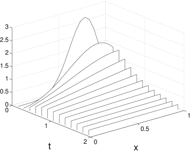
Figure 1: Time evolution of the pdf for a biallelic system as determined from the analytic solution with no mutation and initial condition $x_{0}=0.7$.

(ii) General $M$, no mutations. For general $M$, the solution may be written in the form

$$\mathcal{P}(\underline{u},t|\underline{u}_{0},0)=w(\underline{u}_{0})\sum_{\lambda}\Phi_{\lambda}(\underline{u}_{0})\Phi_{\lambda}(\underline{u})e^{-\lambda t}\,.$$ (19)

as discussed in Section 3. The solution is written in terms of the $\underline{u}$ variables since the problem is separable and so the eigenfunctions are separable. The function $w(\underline{u})$ is given by

$$w(\underline{u})=\prod^{M-1}_{i=1}u_{i}\left(1-u_{i}\right)\,,$$ (20)

and $\lambda$ depends on a set of $M-1$ non-negative integers ${l_{1},l_{2},\ldots,l_{M-1}}$ according to

$$\lambda=\frac{1}{2}L_{M-1}\left(L_{M-1}+1\right)\,,\ \ \ L_{i}=\sum^{i}_{j=1}\left(l_{j}+1\right)\,.$$ (21)

This means that the sum over $\lambda$ in Eq. (19) is in fact an $(M-1)-$dimensional sum.

The property, which we have already remarked upon, that the system with $M-1$ alleles is nested in that with $M$, manifests itself here in the fact that the functions $\Phi_{\lambda}$ are very closely related to the functions which already appear in the two allele solution (17). First of all, since the problem is separable in this coordinate system, they may be written as

$$\Phi_{\lambda}(u_{1},u_{2},\ldots,u_{M-1})=\prod^{M-1}_{i=1}\psi^{(i)}(u_{i})\,.$$ (22)

Each of the factors $\psi^{(i)}$ in this product separately satisfies the same differential equation. We shall derive this equation in Section 3, from which we will learn that $\psi^{(i)}$ depends only on $u_{i}$ and on the integers $l_{i}$ and $L_{i-1}$. Specifically,

$$\psi^{(i)}(u_{i})=\left[c_{l_{i}}(L_{i-1})\right]^{1/2}\left(1-u_{i}\right)^{L_{i-1}}P^{(1,2L_{i-1}+1)}_{l_{i}}(1-2u_{i})\,.$$ (23)

Here the $c_{l_{i}}$ are the analogue of the $c_{l}$ that appeared in Eq. (17), but in this case we have included them in the function $\Phi_{\lambda}$, so that it satisfies the simple orthogonality relation

$$\int{\rm d}\underline{u}\,w(\underline{u})\Phi_{\lambda}(\underline{u})\Phi_{\lambda^{\prime}}(\underline{u})=\delta_{\lambda\,\lambda^{\prime}}\,.$$ (24)

The explicit form of these constants is

$$c_{l_{i}}(L_{i-1})=\frac{(2l_{i}+3+2L_{i-1})(l_{i}+2+2L_{i-1})}{(l_{i}+1)}\,.$$ (25)

The $P^{(1,\beta)}(1-2u)$, now with $\beta=2L_{i-1}+1$, are again Jacobi Polynomials [46].

The general solution for $M>2$ has previously only been found for the case $M=3$. We have checked that our solution agrees with the published result [12] in this case, although the labels on the alleles are permuted between Kimura’s solution and ours ($x_{1}\leftrightarrow x_{3}$) due to a different change of variable being made. We plot this solution for a triallelic system in Fig. 2 at several different times. Just as in the two allele system, the distribution initially spreads out and forms a bell shape, which quickly collapses, and becomes nearly flat, then subsides slowly as probability escapes to the boundaries. Note that the probability deposited on the boundaries is not shown here. Notice also the triangular shape of the region over which the distribution is supported.

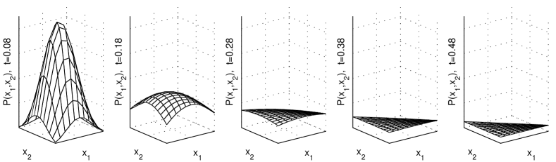
Figure 2: Time evolution of the pdf for a triallelic system as determined from the analytic solution with no mutation and initial condition $x_{1,0}=x_{2,0}=0.33$.

(iii) $M=2$, with mutations. When mutation is present, the solution is again well known [11] for the $M=2$ case. Again, no change of variable is required: $u=x$. Then

$$P(x,t|x_{0},0)=\\ \sum_{l=0}^{\infty}c_{l}x^{\alpha}(1-x)^{\beta}P_{l}^{(\alpha,\beta)}(1-2x_{0})P_{l}^{(\alpha,\beta)}(1-2x)\exp\left\{-\frac{1}{2}l(2R+l-1)t\right\}\;.$$ (26)

The constant $c_{l}$ is given by

$$c_{l}=\frac{\Gamma(2R+l-1)\Gamma(l+1)}{\Gamma(2m_{1}+l)\Gamma(2m_{2}+l)}(2R+2l-1)$$

while $\alpha=2m_{1}-1$, $\beta=2m_{2}-1$ and the parameter $R=m_{1}+m_{2}$.

The $P^{(\alpha,\beta)}_{l}$ are Jacobi polynomials [46]. Unlike the case without mutations, $\alpha\neq\beta$, and they cannot be written in terms of simpler polynomials as in case (i). The function (26) satisfies both the initial and boundary conditions and holds for all $x$ in the interval $[0,1]$, that is, now including the boundaries at $x=0$ and $x=1$. This difference is due to the nature of the boundary conditions in the mutation case, which will be described in detail in Section 3.

For not too small values of $t$, the solution is well approximated by keeping only the first few terms in $l$. In these cases the polynomials do have a relatively simple form, since $P^{(\alpha,\beta)}_{l}(z)$ is a polynomial in $z$ of order $l$. For instance,

$$P^{(\alpha,\beta)}_{0}(z)=1\,,\ \ P^{(\alpha,\beta)}_{1}(z)=\frac{1}{2}[(\alpha+\beta+2)z+\alpha-\beta]\,,\ldots\,.$$ (27)

Also note that once again the natural variable for these polynomials is $z=1-2x$, so that they are defined on the interval $-1\leq z\leq 1$. In terms of the allele $a_{1}$ frequency $x$ and the mutation rates $m_{1}$ and $m_{2}$, these polynomials take the form

$$P^{(2m_{1}-1,2m_{2}-1)}_{0}(1-2x)=1\,,\ \ P^{(2m_{1}-1,2m_{2}-1)}_{1}(1-2x)=2[m_{1}-Rx]\,,\ldots\,.$$ (28)

For concreteness, we plot in Figs. 3 and 4 the time evolution pdfs for biallelic ($M=2$) systems from a fixed initial condition of $x_{0}=0.7$, i.e., that 70% of the population have one particular allele type. In the former case, the mutation rates are low ($m_{1}=m_{2}=0.2$) and one finds a high probability of one allele dominating the population. Conversely, in Fig. 4 which has higher mutation rates $m_{1}=m_{2}=0.8$, the most probable outcome is for both alleles to coexist in the population, as indicated by the peak of the distribution occurring for some value of $x$ far from either boundary. In each of the figures, we compare the distribution obtained from a Monte Carlo simulation of the population dynamics against the analytic result (26) with good agreement.

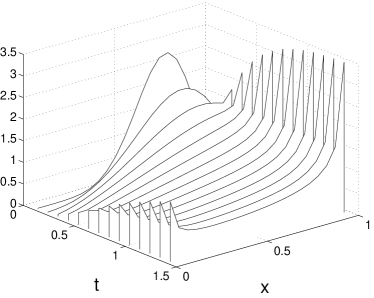
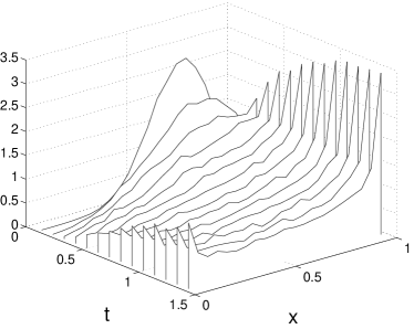
Figure 3: Time evolution of the pdf for a biallelic system as determined from the analytic solution (left) and Monte Carlo simulation (right) with mutation parameters $m_{1}=m_{2}=0.2$ and initial condition $x_{0}=0.7$.

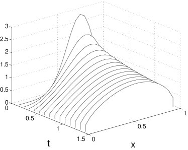
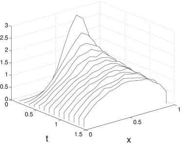
Figure 4: Time evolution of the pdf for a biallelic systems as determined from the analytic solution (left) and Monte Carlo simulation (right) with mutation parameters $m_{1}=m_{2}=0.8$ and initial condition $x_{0}=0.7$.

(iv) General $M$, with mutations. For general $M$, the solution may be written in the form

$$\mathcal{P}(\underline{u},t|\underline{u}_{0},0)=\sum_{\lambda}\Theta_{\lambda}(\underline{u}_{0})\Phi_{\lambda}(\underline{u})e^{-\lambda t}\,.$$ (29)

as discussed in Section 3. Here $\Theta_{\lambda}(\underline{u})$ is the left-eigenfunction of the Kolmogorov equation ($\Phi_{\lambda}(\underline{u})$ being the right-eigenfunction, as usual). Again, $\lambda$ depends on a set of $M-1$ non-negative integers ${l_{1},l_{2},\ldots,l_{M-1}}$, with

$$\lambda=\frac{1}{2}\tilde{L}_{M-1}\left(2R_{1}+\tilde{L}_{M-1}-1\right)\,,\ \ \ \tilde{L}_{i}=\sum^{i}_{j=1}l_{j}\,,\ \ \ R_{1}=\sum^{M}_{i=1}m_{i}\,.$$ (30)

The left-eigenfunction $\Theta_{\lambda}(\underline{u}_{0})$ is equal to $\Phi(\underline{u}_{0})/P_{\rm st}(\underline{u}_{0})$ [40], where $P_{st}(\underline{u}_{0})$ is the stationary pdf. This is equivalent to the form (19), appropriate when there are no mutations, since $(P_{st}(\underline{u}_{0}))^{-1}$ is what is there called the weight function (up to normalisation). Since the problem is separable in this coordinate system, $\Phi$ may again be written as

$$\Phi_{\lambda}(u_{1},u_{2},\ldots,u_{M-1})=\prod^{M-1}_{i=1}\psi^{(i)}(u_{i})\,.$$ (31)

Once again each of the factors $\psi^{(i)}$ is separately a solution of a single differential equation, and depends on $u_{i}$, the integers $l_{M-i}$ and $\tilde{L}_{M-i-1}$ and the mutation rates $m_{i}$. Specifically,

$$\psi^{(i)}(u_{i})=c^{\rm Right}_{l_{M-i}}u_{i}^{\alpha_{i}}\left(1-u_{i}\right)^{\beta_{i}-\tilde{L}_{M-i-1}}P^{(\alpha_{i},\beta_{i})}_{l_{M-i}}(1-2u_{i})\,,$$ (32)

where

$$c^{\rm Right}_{l_{M-i}} = \sqrt{\frac{\Gamma(2R_{i})}{\Gamma(2m_{i})\Gamma(2R_{i+1})}}$$ (33)

$$\times \sqrt{\frac{(2l_{M-i}+\alpha_{i}+\beta_{i}+1)\Gamma(l_{M-i}+1)\Gamma(l_{M-i}+\alpha_{i}+\beta_{i}+1)}{\Gamma(l_{M-i}+\alpha_{i}+1)\Gamma(l_{M-i}+\beta_{i}+1)}}$$

$$\alpha_{i} = 2m_{i}-1$$ (34)

$$\beta_{i} = 2R_{i+1}+2\tilde{L}_{M-i-1}-1$$ (35)

$$R_{i} = \sum_{j=i}^{M}m_{j}\;.$$ (36)

In a similar way, $\Theta_{\lambda}$ may be written as

$$\Theta_{\lambda}(u_{1},u_{2},\ldots,u_{M-1})=\prod^{M-1}_{i=1}\theta^{(i)}(u_{i})\,.$$ (37)

Each $\theta^{(i)}$ depends on $u_{i}$ and on the integer $\tilde{L}_{M-i-1}$ and the mutation constants $R_{i}$ and $m_{i}$. Specifically,

$$\theta^{(i)}(u_{i})=c^{\rm Left}_{l_{M-i}}\left(1-u_{i}\right)^{\tilde{L}_{M-i-1}}P^{(\alpha_{i},\beta_{i})}_{l_{M-i}}(1-2u_{i})\,,$$ (38)

where

$$c^{\rm Left}_{l_{M-i}} = \sqrt{\frac{\Gamma(2m_{i})\Gamma(2R_{i+1})}{\Gamma(2R_{i})}}$$ (39)

$$\times \sqrt{\frac{(2l_{M-i}+\alpha_{i}+\beta_{i}+1))\Gamma(l_{M-i}+1)\Gamma(l_{M-i}+\alpha_{i}+\beta_{i}+1)}{\Gamma(l_{M-i}+\alpha_{i}+1)\Gamma(l_{M-i}+\beta_{i}+1)}}\,.$$

The general solution has previously only been found for the case $M=2$. Our solution agrees with the published result [12] in this case.

2.4 Evolution of the population

We can calculate the time evolution of various statistics of the population. As previously, we present here a summary of the results for ease of reference, deferring detailed calculations to Section 4.

2.4.1 Fixation and extinction

In the absence of mutation, alleles can become extinct since, once they have vanished from the population, there is no mechanism by which they can be replaced. As we have already mentioned, the solution we have derived (19) gives the pdf for all states in the interior. The pdf on a boundary is also given by this equation, so long as this boundary is not the point of fixation of the final allele, since it corresponds to the solution with $M$ reduced by 1. So, for example, one can read off the pdf in, say, the two-dimensional subspace where alleles $a_{1}$ and $a_{2}$ coexist and all others present in the initial population have become extinct since it is just the $M=2$ solution. Kimura [13] finds the large-time form for this quantity given an initial condition comprising $M=3$ alleles using an approach involving moments of the distribution which, as we shall show below, can be found directly from the Kolmogorov equation without recourse to the full solution we have obtained here.

It remains then to determine the fixation probabilities that are excluded from the pdf we have derived. Using a simple argument (outlined below) one can find the probability that a particular allele has fixed by time $t$ by reduction to an equivalent two-allele description, the properties of which are well-known [13]. Using the backward Kolmogorov equation (9), one can find further quantities relating to extinction events. Although some of the formulæ we quote have appeared in the literature before [18, 25] they seem not to be widely known and some were stated without proof. We therefore feel there is some value in reviving them here and giving what is hopefully a clear derivation in this section or in section 4.

Fixation. Define $f_{1}(x_{0},t)$ as the probability that allele $a_{1}$, which had initial frequency $x_{0}$ in a two allele system, has become fixed by time $t$. This is given by [13]

$$f_{1}(x_{0},t)=x_{0}-\frac{1}{2}\sum^{\infty}_{l=0}(-1)^{l}\left[P_{l}(1-2x_{0})-P_{l+2}(1-2x_{0})\right]e^{-(l+1)(l+2)t/2}\,.$$ (40)

Here $P_{l}(z)$ is a Legendre polynomial which is a particular case of the Jacobi polynomials: $P_{l}(z)=P_{l}^{(0,0)}(z)$. Conversely, the probability that $a_{1}$ has become extinct by time $t$ is equal to that of $a_{2}$ become fixed, viz,

$$f_{2}(x_{0},t)=(1-x_{0})-\frac{1}{2}\sum^{\infty}_{l=0}\left[P_{l}(1-2x_{0})-P_{l+2}(1-2x_{0})\right]e^{-(l+1)(l+2)t/2}\;.$$ (41)

Now, consider an initial condition with $M>2$ alleles, divided into two groups $X$ and $Y$. Let now $x$ be the sum of the frequencies of $X$ alleles. We may think of the set of alleles $X$ as a single allele in a two allele system (for instance, $a_{1}$ in the above discussion) and the set $Y$ as the other allele. Then the probability that all of the $Y$ alleles (and possibly some of the $X$ alleles) have become extinct by time $t$ is simply $f_{1}(x_{0},t)$ where $x_{0}$ is the initial combined frequency of $X$ alleles. Similarly, the probability that all of the $X$ alleles are extinct at time $t$, leaving some combination of $Y$ alleles is $f_{2}(x_{0},t)$. Arguments of this kind, where a set of alleles is identified with a single allele in the $M=2$ problem, can be frequently employed to obtain results for the general case of $M$ alleles in terms of those already explicitly calculated for $M=2$.

Coexistence probability. By combining the above reduction to an equivalent two-allele problem with combinatorial arguments, the probability that exactly $r$ alleles coexist at time $t$ can be calculated [18]. The result is

$$\Omega_{r}(\underline{x}_{0},t)=\sum_{s=1}^{r}(-1)^{r-s}\binom{M-s}{r-s}\sum f_{1}(x_{i_{1},0}+\ldots+x_{i_{s},0},t)\,,$$ (42)

where $r$ can take any value from $1$ up to $M$, and the second summation is over all subsets of size $s$ drawn from the $M$ alleles. It is a simple matter to use this formula to calculate the mean number of coexisting alleles at time $t$.

In Fig. 5, we compare the time-dependent probabilities for $1\leq r\leq 4$ alleles to be present in a system initially comprising $M=4$ alleles given by the exact formula (42) and as obtained from a Monte-Carlo simulation with the allele frequencies initially equal. We also show the evolution of the mean number of coexisting alleles from starts with $M=3$ and $M=4$ alleles. In both cases, the exact formulæ correspond extremely well with the simulations, illustrating the utility of the diffusion approximation to the discrete population dynamics.

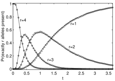
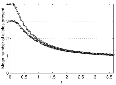
Figure 5: Probabilities that exactly $r$ alleles are present as a function of time for $r=1,2,3,4$ in a system with 4 alleles initially. Expected number of alleles present as a function of time for systems with 3 and 4 alleles initially present (right). Symbols are Monte Carlo simulation data, solid curves are analytic calculations.

Mean time to the $r$th extinction. By solving the appropriate backward Kolmogorov equation, one can straightforwardly find the mean time to the first (and only) extinction event among two alleles to be

$$\tau(x_{0})=-2\left[x_{0}\ln x_{0}+(1-x_{0})\ln(1-x_{0})\right]\,.$$ (43)

A combinatorial analysis, performed in [18] and which we will summarise in Section 4.1, reveals the mean time to the $r^{\rm th}$ extinction can be calculated from an $M=2$ result. One finds

$$\tau_{r}(M)=-2\sum_{s=r}^{M-1}(-1)^{s-r}\binom{s-1}{r-1}\sum[(x_{i_{1},0}+\ldots+x_{i_{k},0})\ln(x_{i_{1},0}+\ldots+x_{i_{s},0})]\;,$$ (44)

where $x_{i_{k},0}$ is the initial fraction of allele $a_{k}$ present in the system. The second sum is over all possible $s$-subsets $\{i_{1},i_{2},\ldots,i_{s}\}$ of the $M$ alleles initially present in the population.

Probability of a particular sequence of extinctions. Not all extinction probabilities can be calculated by reduction to an equivalent a two-allele problem. A notable example is the probability that allele $a_{i_{1}}$ goes extinct first, followed by $a_{i_{2}},a_{i_{3}},\ldots,a_{i_{M-1}}$ leaving only $a_{i_{M}}$ in the final population, since in this case we ask for all, rather than just some of a subset to be present in the population at a given time. This probability is given by

$$Q_{i_{1},i_{2},\ldots,i_{M-1}}(\underline{x})=x_{i_{M},0}\frac{x_{i_{M-1},0}}{1-x_{{i_{M}},0}}\frac{x_{i_{M-2},0}}{1-x_{{i_{M}},0}-x_{i_{M-1},0}}\cdots\\ \cdots\frac{x_{{i_{2}},0}}{1-x_{{i_{M}},0}-x_{i_{{M-1},0}}-\cdots-x_{{i_{3}},0}}$$ (45)

in which $x_{i,0}$ is the initial frequency of allele $a_{i}$ in the population. This result appears in [19], albeit without an explicit derivation. We shall provide one in Section 4.1.

First-passage probability. An immediate consequence of the previous result is the probability that a particular allele, $a_{i}$ is the first to become extinct, that is, at a time when all other alleles have a nonzero frequency. This is obtained by summing (45) over all possible sequences of extinctions in which $a_{i}$ goes extinct first. For example, when the initial number of alleles $M=3$, the probability that $a_{1}$ goes extinct first can be found by summing over the cases $(i_{1},i_{2},i_{3})=(1,2,3),(1,3,2)$ in (45). One finds

$$Q_{1}(x_{1,0},x_{2,0})=x_{2,0}\frac{x_{3,0}}{1-x_{2,0}}+x_{3,0}\frac{x_{2,0}}{1-x_{3,0}}\,,$$

where $x_{3,0}=1-x_{1,0}-x_{2,0}$. This agrees with the result in [18]. By a similar method, one could determine the probability for allele $a_{i}$ to be the second to go extinct or any other quantity of this type.

2.4.2 Stationary distribution

When mutations are absent, we see from (40) that allele $a_{i}$ fixes with a probability equal to its initial frequency in the population. Hence in this case, the stationary distribution

$$P^{\ast}(\underline{x})=\lim_{t\to\infty}P(\underline{x},t|\underline{x}_{0},0)$$ (46)

is zero everywhere except at those points that correspond to fixation of a single allele.

On the other hand, when all the mutation rates $m_{i}$ at which all alleles $a_{j},j\neq i$ mutate to $a_{i}$ are nonzero, the stationary distribution is nonzero everywhere. Furthermore, this distribution is reached from any initial condition and takes the well-known form [4, 38]

$$P^{\ast}(\underline{x})=\Gamma(2R)\prod_{i=1}^{M}\frac{x_{i}^{2m_{i}-1}}{\Gamma(2m_{i})}\;,$$ (47)

where in keeping with the 2 allele case $R=R_{1}=\sum_{j=1}^{M}m_{j}$. Recall that the frequency $x_{M}$ is implied through the normalisation $\sum_{i=1}^{M}x_{i}=1$.

2.4.3 Moments and Heterozygosity

One way to calculate moments of the distribution is to integrate the exact solution we have obtained above. However, it is also possible to derive differential equations for the moments in terms of lower-order moments from the Kolmogorov equation, a procedure that leads more quickly to simple, exact expressions for low-order moments. We quote some examples for general $M$ here, noting that previously results for $M=2$ and $3$ without mutations have previously appeared in [13, 11] and for $M=2$ with mutations in [47, 38]. It is also worth remarking that by calculating moments, Kimura reconstructed the solution for the pdf for the case $M=3$ and no mutations [13].

No mutations. When mutations are absent, the mean of $x_{i}$ is conserved by the dynamics, i.e.,

$$\langle x_{i}(t)\rangle=x_{i,0}\,.$$ (48)

Meanwhile, the variance changes with time as

$$\langle\langle x_{i}^{2}(t)\rangle\rangle_{x_{i}(0)=x_{i,0}} \equiv \langle x_{i}^{2}(t)\rangle_{x_{i}(0)=x_{i,0}}-\left(\langle x_{i}(t)\rangle_{x_{i}(0)=x_{i,0}}\right)^{2}$$ (49)

$$= x_{i,0}(1-x_{i,0})\left(1-e^{-t}\right)\;.$$

This result is clear, at least in the case $M=2$. The delta-function initial condition has zero variance, and the stationary distribution comprises delta-functions at $x=0$ and $x=1$ with weights $(1-x_{0})$ and $x_{0}$ respectively. For the latter one then has $\langle x^{2}\rangle=(1-x_{0})\cdot 0+x_{0}\cdot 1=x_{0}$ and so $\langle\langle x^{2}\rangle\rangle=x_{0}(1-x_{0})$.

The covariance, which does not appear in the two allele system is:

$$\langle\langle x_{i}x_{j}\rangle\rangle\equiv\langle x_{i}x_{j}\rangle-\langle x_{i}(t)\rangle\langle x_{j}(t)\rangle=x_{i,0}x_{j,0}(e^{-t}-1)\,.$$

With mutations. Crow and Kimura [47] give moments only for the biallelic case, and then in terms of hypergeometric functions. We provide simpler results in explicit form here, again for any $M$. The mean frequency of any allele behaves as

$$\langle x_{i}(t)\rangle=\frac{m_{i}}{R}+\left(x_{i,0}-\frac{m_{i}}{R}\right)e^{-Rt}=\eta_{i}+\zeta_{i}e^{-Rt}\;,$$ (50)

where

$$\eta_{i}=\frac{m_{i}}{R},\ \ \ \zeta_{i}=x_{i,0}-\frac{m_{i}}{R}\,.$$ (51)

The mean (50) exponentially approaches the fixed point of the deterministic motion. Recalling that $R=\sum_{i}m_{i}$, we see in Eq. (5) the function $A_{i}(x)$ vanishes at the point $x=m_{i}/R\;\forall i$.

The variance is more complicated:

$$\langle\langle x_{i}^{2}(t)\rangle\rangle=\frac{\eta_{i}(1-\eta_{i})}{(2R+1)}+\frac{\zeta_{i}(1-2\eta_{i})}{(R+1)}e^{-Rt}-\zeta_{i}^{2}e^{-2Rt}\\ -\left\{\frac{\eta_{i}(1-\eta_{i})}{(2R+1)}+\frac{\zeta_{i}(1-2\eta_{i})}{(R+1)}-\zeta_{i}^{2}\right\}e^{-(2R+1)t}\,.$$ (52)

As $t\to\infty$, this converges to the limit

$$\langle\langle x^{2}(t)\rangle\rangle_{t\to\infty}=\frac{\eta_{i}(1-\eta_{i})}{(2R+1)}=\frac{m_{i}(R-m_{i})}{R^{2}(2R+1)}\;.$$ (53)

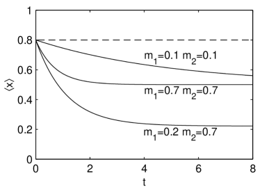
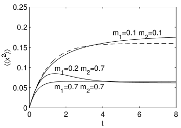
Figure 6: Solid lines: Time evolution of the mean (left) and variance (right) for a biallelic system for three different mutation parameter combinations, and with $x_{0}=0.8$. Dashed lines: Evolution of mean and variance when mutation is absent.

In Fig. 6 we show the mean and variance as a function of time in the biallelic case, for three different pairs of mutation parameters. The mean approaches the stationary distribution value exponentially, at a faster rate the larger the values of the mutation parameters. When $m_{1}=m_{2}$, the variance rises asymptotically to the stationary limit, again faster when the mutation parameters are larger. Notice that for small values of $m_{1}$ and $m_{2}$, the final variance is close to that when no mutations occur, while the larger the mutation parameters become, the narrower the final distribution. When the parameters are unequal, the variance can reach a maximum value before descending slowly to the final limit.

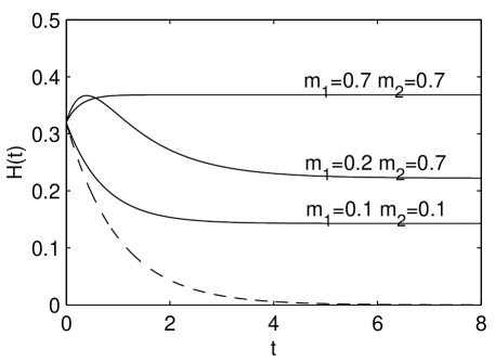
Figure 7: The time development of the heterozygosity with two alleles, for the case with no mutations (dashed curve) and for three different cases of mutation (solid curves), $x_{0}=0.8$ in each case.

The covariance (with $i\neq j$) is

$$\langle\langle x_{i}x_{j}\rangle\rangle \equiv \langle x_{i}x_{j}\rangle-\langle x_{i}\rangle\langle x_{j}\rangle$$ (54)

$$= -\frac{\eta_{i}\eta_{j}}{(2R+1)}-\frac{(\eta_{i}\zeta_{j}+\eta_{j}\zeta_{i})}{(R+1)}e^{-Rt}-\zeta_{i}\zeta_{j}e^{-2Rt}$$

$${}+\left\{\frac{\eta_{i}\eta_{j}}{(2R+1)}+\frac{(\eta_{i}\zeta_{j}+\eta_{j}\zeta_{i})}{(R+1)}+\zeta_{i}\zeta_{j}\right\}e^{-(2R+1)t}\,.$$

Heterozygosity. As asserted by Kimura [13], in the absence of mutation the heterozygosity decays as $e^{-t}$ regardless of the initial number of alleles. The heterozygosity is the probability that two alleles chosen at random from the population will be different. When there are multiple alleles, this probability can be calculated from the first and second moments using

$$H(t)=\sum_{i}[2(\langle x_{i}\rangle-\langle x_{i}^{2}\rangle)-\sum_{j\neq i}\langle x_{i}x_{j}\rangle]\;.$$ (55)

When expressions for the various moments are substituted into this expression, it is found that, in the absence of mutations, the constant terms cancel, leaving only terms decaying as $e^{-t}$. Therefore we have

$$H(x_{0},t)=H_{0}e^{-t}\;,$$ (56)

where we find $H_{0}=2\sum_{i}(x_{i,0}-x_{i,0}^{2})-\sum_{i}\sum_{j\neq i}x_{i,0}x_{j,0}$. Kimura derived this result from the expected change in $H$ with each generation.

The calculation with mutation present, however, does not give such a simple result. The heterozygosity can also be found for any number of alleles when mutation is present. However, the form becomes increasingly complicated as $M$ increases. Therefore we give as an example only the two allele result here:

$$H(x_{0},t) \equiv 2\langle x(1-x)\rangle$$ (57)

$$= \frac{4m_{1}m_{2}}{R(2R+1)}-2\left(\frac{m_{2}-m_{1}}{R+1}\right)\left(x_{0}-\frac{m_{1}}{R}\right)e^{-Rt}$$

$${}-2\left[x_{0}^{2}-\left(\frac{2m_{1}+1}{R+1}\right)\left(x_{0}-\frac{m_{1}}{2R+1}\right)\right]e^{-(2R+1)t}\,.$$

This is plotted in Fig. 7. We see that the presence of mutation between the two alleles maintains the heterozygosity at a finite level.

3 Solution of the Kolmogorov equation

In this section we will derive the solution of the Kolmogorov equation (12), which was given in Section 2.3. In particular we will derive the differential equation that is satisfied by every single one of the factors $\psi^{(i)}(u_{i})$ that appear in the eigenfunction $\Phi_{\lambda}(\underline{u})$ in Eq. (22) which applies when no mutations occur. We shall also present the more general differential equation that must be solved to determine the corresponding factors in (31) that give the eigenfunctions when mutations are present. The more technical points of the discussion are relegated to Appendices B and C, in order to avoid interrupting the flow of the arguments.

3.1 Change of variables

It is worthwhile to recall briefly the derivation of the Kolmogorov equation itself, since it will turn out that the most efficient way of changing from the $\underline{x}$ variables to the $\underline{u}$ variables is go back to an early stage of this derivation. The starting point for the derivation is the Chapman-Kolmogorov equation which is one of the defining equations for Markov processes:

$$P(\underline{x},t^{\prime}|\underline{x}_{0},0)=\int{\rm d}\underline{x}^{\prime}P(\underline{x},t^{\prime}|\underline{x}^{\prime},t)\,P(\underline{x}^{\prime},t|\underline{x}_{0},0)\,.$$ (58)

If we take $t^{\prime}=t+\Delta t$ and expand

$$P(\underline{x},t+\Delta t|\underline{x}^{\prime},t)\,$$ (59)

in powers of $\Delta x_{i}(t)=x_{i}(t+\Delta t)-x_{i}(t)$, we find—in the limit $\Delta t\to 0$—the Kramers-Moyal expansion for $P(\underline{x},t|\underline{x}_{0},0)$ [40]:

$$\frac{\partial P}{\partial t}=\sum^{\infty}_{m=1}\,\frac{(-1)^{m}}{m!}\frac{\partial^{m}}{\partial x_{i_{1}}\ldots\partial x_{i_{m}}}\left\{\alpha_{i_{1}\ldots i_{m}}(\underline{x})P\right\}\,.$$ (60)

Here the $\alpha_{i_{1}\ldots i_{m}}(\underline{x})$ are the jump moments defined through the relation

$$\left\langle\Delta x_{i_{1}}(t)\Delta x_{i_{2}}(t)\ldots\Delta x_{i_{m}}(t)\right\rangle_{\underline{x}(t)=\underline{x}}=\alpha_{i_{1}\ldots i_{m}}(\underline{x})\Delta t+\mathcal{O}(\Delta t)^{2}\,.$$ (61)

The angle brackets are averages over realisations of the process $\underline{x}(t)$; $\underline{x}(t)$ is a stochastic process, whereas $\underline{x}_{0}$ and $\underline{x}$ are simply the initial and final states.

So far very little has been assumed other than the Markov property of the stochastic process. The Markov nature of the process follows from the fact that the sampling of gametes from the gamete pool depends only on its current state, and not on its past history. If we assume that no deterministic forces are present, only the random mating process, then $\langle\Delta x_{i_{1}}(t)\rangle_{\underline{x}(t)=\underline{x}}=0$. If deterministic forces are present, then there will be an $\mathcal{O}(\Delta t)$ contribution to $\langle\Delta x_{i_{1}}(t)\rangle_{\underline{x}(t)=\underline{x}}$ which is equal to $({\rm d}x_{i_{1}}/{\rm d}t)|_{\rm det}\,\Delta t$. Here $({\rm d}x_{i_{1}}/{\rm d}t)|_{\rm det}$ is the rate of change of $x_{i_{1}}$ in the deterministic ($N\to\infty$) limit. The higher jump moments reflect the statistics of the sampling process. In the case of two alleles this is binomial and so the second jump moment is proportional to $x(1-x)$, which is the variance of this distribution. Within the diffusion approximation, a unit of time is taken to be $2N$ generations, so that the time between generations is $\Delta t=1/(2N)$. This implies that all jump moments higher than the second are higher order in $\Delta t$. This gives the results (5) and (6). For the case of general $M$, the multinomial distribution applies, which again means that the $\alpha_{i_{1}\ldots i_{m}}(\underline{x})$ for $m>2$ vanish, and the second order jump moment is given by (4), up to a factor of $2$.

This is the briefest summary of the derivation of Eq. (8). We refer the reader to [40] for a fuller account. However, the above discussion is sufficient for our purposes, which is to note that the derivation involving Eqs. (58)-(61) may be carried out for any coordinate system, and specifically in the coordinate system $\underline{u}=(u_{1},u_{2},\ldots,u_{M-1})$ for which the Kolmogorov equation is separable. In this case the Kramers-Moyal expansion for $\mathcal{P}(\underline{u},t|\underline{u}_{0},0)$ is

$$\frac{\partial\mathcal{P}}{\partial t}=\sum^{\infty}_{m=1}\,\frac{(-1)^{m}}{m!}\frac{\partial^{m}}{\partial u_{i_{1}}\ldots\partial u_{i_{m}}}\left\{\tilde{\alpha}_{i_{1}\ldots i_{m}}(\underline{u})\mathcal{P}\right\}\,,$$ (62)

where $\tilde{\alpha}_{i_{1}\ldots i_{m}}(\underline{u})$ are the jump moments in the new coordinate system:

$$\left\langle\Delta u_{i_{1}}(t)\Delta u_{i_{2}}(t)\ldots\Delta u_{i_{m}}(t)\right\rangle_{\underline{u}(t)=\underline{u}}=\tilde{\alpha}_{i_{1}\ldots i_{m}}(\underline{u})\Delta t+\mathcal{O}(\Delta t)^{2}\,.$$ (63)

The most straightforward way of deriving the Kolmogorov equation in the $\underline{u}$ variables is to start from Eq. (62) and determine the $\tilde{\alpha}_{i_{1}\ldots i_{m}}(\underline{u})$ by relating them to the known $\alpha_{i_{1}\ldots i_{m}}(\underline{x})$. This is carried out in Appendix B and the result is the equations (12) and (13).

3.2 Separation of variables

The next step in the solution of the Kolmogorov equation is to separate out the time and $u_{i}$ coordinates. That is, we write the general solution as a linear combination of such solutions:

$$\mathcal{P}(\underline{u},t|\underline{u}_{0},0)=\sum_{\lambda}a_{\lambda}(\underline{u}_{0})\Phi_{\lambda}(\underline{u})e^{-\lambda t}\,,$$ (64)

where the function $\Phi_{\lambda}(\underline{u})$ satisfies

$$\sum_{i}\frac{1}{\prod_{j<i}(1-u_{j})}\,\frac{\partial}{\partial u_{i}}\left\{\left(R_{i}u_{i}-m_{i}\right)+\frac{1}{2}\frac{\partial}{\partial u_{i}}\left[u_{i}(1-u_{i})\right]\right\}\Phi_{\lambda}(\underline{u})=-\lambda\Phi_{\lambda}(\underline{u})$$ (65)

and $R_{i}=\sum_{j=i}^{M}m_{j}$. We may apply initial conditions directly on (64):

$$\delta(\underline{u}-\underline{u}_{0})=\sum_{\lambda}a_{\lambda}(\underline{u}_{0})\Phi_{\lambda}(\underline{u})\,.$$ (66)

By assuming the orthogonality relation

$$\int{\rm d}\underline{u}\,w(\underline{u})\Phi_{\lambda}(\underline{u})\Phi_{\lambda^{\prime}}(\underline{u})=\delta_{\lambda\lambda^{\prime}}\,,$$ (67)

where $w(\underline{u})$ is an appropriate weight function, we then have that $a_{\lambda}(\underline{u})=w(\underline{u})\Phi_{\lambda}(\underline{u})$ and so

$$\mathcal{P}(\underline{u},t|\underline{u}_{0},0)=w(\underline{u}_{0})\sum_{\lambda}\Phi_{\lambda}(\underline{u}_{0})\Phi_{\lambda}(\underline{u})e^{-\lambda t}\,.$$ (68)

To determine $\Phi_{\lambda}(\underline{u})$ we have in principle to solve the partial differential equation (65) in $n=M-1$ variables. We will now prove that this equation is separable in the $\underline{u}$ variables. For clarity we will start where mutation does not take place (that is, omit the factor $(R_{i}u_{i}-m_{i})$ in (65))—the argument goes through in an identical fashion when this term is present, as we will discuss later.

When $n=1\ (M=2)$ $\Phi_{\lambda}(\underline{u})$ satisfies the equation

$$\frac{1}{2}\frac{{\rm d}^{2}}{{\rm d}u^{2}_{1}}\left[u_{1}(1-u_{1})\Phi_{\lambda^{(1)}}(u_{1})\right]=-\lambda^{(1)}\Phi_{\lambda^{(1)}}(u_{1})\,,$$ (69)

where we have introduced the superscript $(1)$ on to the eigenvalue $\lambda$ to identify it as belonging to the $n=1$ problem. This ordinary differential equation may be solved in a straightforward fashion as we discuss in the next subsection below.

When $n=2\ (M=3)$ $\Phi_{\lambda}(\underline{u})$ satisfies the equation

$$\frac{1}{2}\frac{\partial}{\partial u^{2}_{1}}\left[u_{1}(1-u_{1})\Phi_{\lambda^{(2)}}(u_{1},u_{2})\right] +$$

$$\frac{1}{2}\,\frac{1}{1-u_{1}}\,\frac{\partial}{\partial u^{2}_{2}}\left[u_{2}(1-u_{2})\Phi_{\lambda^{(2)}}(u_{1},u_{2})\right] = -\lambda^{(2)}\Phi_{\lambda^{(2)}}(u_{1},u_{2})\,.$$ (70)

We look for a separable solution of the form $\Phi_{\lambda^{(2)}}(u_{1},u_{2})=\psi(u_{1})\phi_{\lambda^{(1)}}(u_{2})$ where

$$\frac{1}{2}\frac{{\rm d}^{2}}{{\rm d}u^{2}_{2}}\left[u_{2}(1-u_{2})\phi_{\lambda^{(1)}}(u_{2})\right]=-\lambda^{(1)}\phi_{\lambda^{(1)}}(u_{2})\,,$$

that is, $\phi_{\lambda^{(1)}}(u_{1})$ satisfies the equation corresponding to the $n=1$ problem. It is straightforward to show that a separable solution exists if $\psi(u_{1})$ satisfies the equation

$$\frac{1}{2}\frac{{\rm d}^{2}}{{\rm d}u^{2}_{1}}\left[u_{1}(1-u_{1})\psi_{\lambda^{(2)};\lambda^{(1)}}(u_{1})\right]=\left\{-\lambda^{(2)}+\frac{\lambda^{(1)}}{(1-u_{1})}\right\}\psi_{\lambda^{(2)};\lambda^{(1)}}(u_{1})\,.$$ (71)

We have introduced the subscript $\lambda^{(2)};\lambda^{(1)}$ on $\psi(u_{1})$ to show that it depends on both the eigenvalues of the $n=2$ and the $n=1$ problems. As we will see, it is a remarkable fact that the solution of the problem with $M=n+1$ alleles only involves the function $\psi$ appearing in Eq. (71). Since $\phi_{\lambda^{(1)}}(u_{2})$ may also be written as $\psi_{\lambda^{(1)};0}$ we may write the separable form of the solution in the $n=2$ case as

$$\Phi_{\lambda^{(2)}}(u_{1},u_{2})=\psi_{\lambda^{(2)};\lambda^{(1)}}(u_{1})\psi_{\lambda^{(1)};0}(u_{2})\,.$$ (72)

We can now prove that the general case of $M=n+1$ alleles is separable as follows. We look for a solution of (65) of the form

$$\Phi_{\lambda^{(n)}}(u_{1},u_{2},\ldots,u_{n})=\psi(u_{1})\Phi_{\lambda^{(n-1)}}(u_{2},\ldots,u_{n})\,,$$

where $\Phi_{\lambda^{(n-1)}}(u_{2},\ldots,u_{n})$ is the solution of (65) with $n-1$ alleles, but with the replacements $u_{1}\to u_{2},u_{2}\to u_{3},\ldots,u_{n-1}\to u_{n}$. By explicit substitution into (65) it is not difficult to demonstrate this, and to find that $\psi(u_{1})$ satisfies Eq. (71), where now $\lambda^{(2)}$ and $\lambda^{(1)}$ are replaced by $\lambda^{(n)}$ and $\lambda^{(n-1)}$ respectively. Therefore we have shown that

$$\Phi_{\lambda^{(n)}}(u_{1},u_{2},\ldots,u_{n})=\psi_{\lambda^{(n)};\lambda^{(n-1)}}(u_{1})\Phi_{\lambda^{(n-1)}}(u_{2},\ldots,u_{n})\,.$$ (73)

This shows that if the $n-1$ allele problem is separable, then the $n$ allele problem is separable. But Eq. (72) shows that the $n=2$ problem is separable, and so by induction the problem for general $n$ is separable. The explicit solution is

$$\Phi_{\lambda^{(n)}}(u_{1},u_{2},\ldots,u_{n})=\prod^{n}_{i=1}\psi_{\lambda^{(n+1-i)};\lambda^{(n-i)}}(u_{i})\,,$$ (74)

where $\lambda^{(0)}\equiv 0$ and where $\psi_{\lambda;\lambda^{\prime}}(u)$ satisfies the equation

$$\frac{1}{2}\frac{{\rm d}^{2}}{{\rm d}u^{2}}\left[u(1-u)\psi_{\lambda;\lambda^{\prime}}(u)\right]=\left\{-\lambda+\frac{\lambda^{\prime}}{(1-u)}\right\}\psi_{\lambda;\lambda^{\prime}}(u)\,.$$ (75)

Thus we have finally shown that in order to obtain the eigenfunction $\Psi_{\lambda^{(n)}}(u_{1},\ldots,u_{n})$ it is necessary only to solve this single ordinary differential equation for general $\lambda$ and $\lambda^{\prime}$. The full eigenfunction is then just a product of solutions of this equation.

A similar equation arises from an analogous argument when mutation is included, that is, the factor $(R_{i}u_{i}-m_{i})$ is restored into Eq. (65): all that is required is to make the substitution

$$\frac{1}{2}\frac{\partial}{\partial u_{i}}\left[u_{i}(1-u_{i})\right]\longrightarrow\frac{1}{2}\frac{\partial}{\partial u_{i}}\left[u_{i}(1-u_{i})\right]+\left(R_{i}u_{i}-m_{i}\right)$$

in the above argument. The only difference is that now the function $\psi$ explicitly depends on $i$ because of the existence of the terms $R_{i}$ and $m_{i}$. Thus the results corresponding to Eqs. (74) and (75) are:

$$\Phi_{\lambda^{(n)}}(u_{1},u_{2},\ldots,u_{n})=\prod^{n}_{i=1}\psi^{(i)}_{\lambda^{(n+1-i)};\lambda^{(n-i)}}(u_{i})\,,$$ (76)

where $\psi^{(i)}_{\lambda;\lambda^{\prime}}(u_{i})$ satisfies the equation

$$\frac{{\rm d}}{{\rm d}u_{i}}\left[\left(R_{i}u_{i}-m_{i}\right)\psi^{(i)}_{\lambda;\lambda^{\prime}}(u_{i})\right] + \frac{1}{2}\frac{{\rm d}^{2}}{{\rm d}u^{2}_{i}}\left[u_{i}(1-u_{i})\psi^{(i)}_{\lambda;\lambda^{\prime}}(u_{i})\right]$$ (77)

$$= \left\{-\lambda+\frac{\lambda^{\prime}}{(1-u_{i})}\right\}\psi^{(i)}_{\lambda;\lambda^{\prime}}(u_{i})\,.$$

The rest of this section will be devoted to solving the ordinary differential equations (75) and (77) subject to the boundary conditions of the problem.

3.3 Solution of the ordinary differential equations

3.3.1 Reduction to a standard form

To solve the ordinary differential equation (77) (which includes the less general Eq. (75) as a special case) it is useful to cast it in a standard form. To this end, we introduce the function $f^{(i)}_{\lambda;\lambda^{\prime}}(u_{i})$ by writing

$$\psi^{(i)}_{\lambda;\lambda^{\prime}}(u_{i})=\left(1-u_{i}\right)^{\gamma_{i}}\,f^{(i)}_{\lambda;\lambda^{\prime}}(u_{i})\,,$$ (78)

where $\gamma_{i}$ is a constant which is to be appropriately chosen shortly. Substituting Eq. (78) into Eq. (77) one finds (dropping the subscripts and superscripts on $f$)

$$u_{i}(1-u_{i})f^{\prime\prime}+2\left[(1-m_{i})+(R_{i}-(\gamma_{i}+2)u_{i}\right]f^{\prime}\\ +\left[2\lambda-(\gamma_{i}+1)(\gamma_{i}+2)+2R_{i}(\gamma_{i}+1)\right]f\\ =\frac{\left[2\lambda^{\prime}-\gamma_{i}(\gamma_{i}+1)-2\gamma_{i}(m_{i}-R_{i})\right]}{1-u_{i}}\,f\,.$$ (79)

We will choose $\gamma_{i}$ so that the term involving $(1-u_{i})$ in the denominator vanishes, that is, we ask that

$$\gamma_{i}\left(\gamma_{i}+1+2m_{i}-2R_{i}\right)=2\lambda^{\prime}\,.$$ (80)

This is a quadratic equation for $\gamma_{i}$, but it is simple to see that if $\gamma_{i}$ is one solution, the second one is simply $\gamma_{i}^{\prime}=2R_{i}-2m_{i}-1-\gamma_{i}$. It will turn out that either choice leads to the same form for $\psi^{(i)}_{\lambda;\lambda^{\prime}}(u_{i})$.

If we choose $\gamma_{i}$ to satisfy Eq. (80), then Eq. (79) has the form

$$u_{i}(1-u_{i})f^{\prime\prime}+\left[c-(a+b+1)u_{i}\right]f^{\prime}-abf=0\,,$$ (81)

where

$$c=2(1-m_{i});\ \ a+b=2\gamma_{i}+3-2R_{i};\ \ ab=(\gamma_{i}+1)(\gamma_{i}+2)-2R_{i}(\gamma_{i}+1)-2\lambda\,.$$ (82)

The solution of the equation has now been reduced to a standard form, since Eq. (81) is the hypergeometric equation [46], whose solutions are hypergeometric functions $F(a,b,c,z)$. The details of the analysis of this equation are given in Appendix C; here we only describe the general features and specific form of the solution, without going into their derivation. That is, we find the constants $\gamma_{i}$ and $\lambda$. In the following discussion it is convenient to treat the cases where mutations do and do not occur separately.

3.3.2 Solution in the absence of mutations

We begin with the situation where mutations are absent, and so the pdf is found by solving Eq. (81), but where now

$$c=2;\ \ a+b=2\gamma_{i}+3;\ \ ab=(\gamma_{i}+1)(\gamma_{i}+2)-2\lambda\,.$$ (83)

The $\gamma_{i}$ are chosen so that $\gamma_{i}(\gamma_{i}+1)=2\lambda^{\prime}$. We begin the discussion, for orientation, by assuming that only two alleles are present. This amounts to solving Eq. (69) or Eq. (75) with $\lambda^{\prime}=0$, and the solution is therefore the function $\psi_{\lambda^{(1)};0}(u_{1})=\phi_{\lambda^{(1)}}(u_{1})$. This function also appears in the solution for arbitrary $M$, given by Eq. (74), and so this result is also required in the general case.

Since in this simple case of two alleles $\lambda^{\prime}=0$, it follows that $\gamma_{1}=0$ or $\gamma_{1}=-1$. As discussed in Appendix C, either choice gives the same solution, and we therefore take $\gamma_{1}=0$. We have now only to solve the second order ordinary differential equation (81) subject to boundary conditions at $u_{1}=0$ and $u_{1}=1$. As is familiar in such problems [48], the general solution is first expressed as a linear combination of two independent solutions. One of these is ruled out by one of the boundary conditions (e.g. the one at $u_{1}=0$) and the application of the other boundary condition constrains a function of $\lambda$ to be an integer; in our case one finds $a=-l,\ l=0,1,\ldots$. Details are in Appendix C, but we do wish to mention the nature of the boundary conditions here. Technically [42] these are exit boundary conditions which means that all the probability which diffuses to the boundary is “extracted” from the interval $(0,1)$. Naïvely, one might imagine that it is appropriate to impose absorbing boundary conditions, i.e., that the pdf vanishes at $u_{1}=0$ and $u_{1}=1$. However, since the diffusion coefficient, defined in Eq. (1), vanishes on the boundaries the diffusion equation itself imposes some sort of absorption. A more careful mathematical analysis, such as the informal argument presented in Appendix A, reveals that the appropriate constraint on the eigenfunctions is that they should diverge less rapidly than a square-root at both boundaries.

The result $a=-l$ imposed by the boundary conditions together with the definitions (83) imply that $b=l+3,ab=-l^{2}-3l$ and so

$$\lambda=\frac{1}{2}\left(l+1\right)\left(l+2\right)\,.$$ (84)

The solutions of the differential equation will be labelled by the integer $l$ and consist of polynomials of order $l$. These have already been mentioned in Section 2 (Eq. (17)), whilst more technical information can be found in Appendix C.

Now we can move on to the solution for general $M$. As explained above it is sufficient to solve Eq. (75) where $\lambda^{\prime}$ is given by the $\lambda$ found in the solution of the $M-1$ allele problem. We have seen that for $M=2$, this is given by (84), and so this will be the $\lambda^{\prime}$ for the $M=3$ problem. We will see that this will have the general structure $(L+1)(L+2)/2$, where $L$ is an integer, and therefore we take this form for $\lambda^{\prime}$. From the way that the $M-1$ problem is embedded in the $M$ allele problem, we always have only to solve the $u_{1}$ equation and so we need to determine $\gamma_{1}$. This is determined by the equation $\gamma_{1}(\gamma_{1}+1)=2\lambda^{\prime}$ from which we see that $\gamma_{1}=L+1$ or $\gamma_{1}=-L-2$. Again, both give the same result and so we take the former. Applying the boundary conditions again gives $a=-l$, with $l=0,1,\ldots$—see Appendix C for the details. Using Eq. (83) one sees that $b=2L+l+5$ and so

$$\lambda=\frac{1}{2}\left(L+l+2\right)\left(L+l+3\right)=\frac{1}{2}\left(L^{\prime}+1\right)\left(L^{\prime}+2\right)\,,$$ (85)

where $L^{\prime}=L+l+1$. This justifies the choice for $\lambda^{\prime}$.

In summary, we have found that $\lambda^{(1)}=(l_{1}+1)(l_{1}+2)/2$, $\lambda^{(2)}=(l_{1}+l_{2}+2)(l_{1}+l_{2}+3)/2,\ldots$. If we define

$$L_{i}\equiv\sum_{j\leq i}\left(l_{j}+1\right)\,,$$ (86)

then $\lambda^{(i)}=L_{i}(L_{i}+1)/2$, and we have recovered (21). The general solution is given by Eqs. (19)-(25) and discussed further in Appendix C.

3.3.3 Solution with mutations

When mutations are present we have to solve Eq. (81) subject to the general set of parameter values given by Eq. (82). While it is true that this slightly complicates the analysis as compared with that of the mutation-free case, the most significant change is the nature of the boundary conditions. The introduction of mutations in the way we have done here renders the boundaries reflecting, which are defined as having no probability current through them. The current $J_{i}(\underline{u},t)$ satisfies the continuity equation [40, 41]

$$\frac{\partial\mathcal{P}}{\partial t}+\sum^{M-1}_{i=1}\frac{\partial J_{i}}{\partial u_{i}}=0\,,$$ (87)

where (compare with Eqs. (12) and (13)),

$$J_{i}(\underline{u},t) = \left[\mathcal{A}_{i}(\underline{u})\mathcal{P}(\underline{u},t)\right]-\frac{\partial}{\partial u_{i}}\left[\mathcal{D}_{i}(\underline{u})\mathcal{P}(\underline{u},t)\right]$$ (88)

$$= \frac{1}{\prod_{j<i}(1-u_{j})}\left\{\left(m_{i}-R_{i}u_{i}\right)\mathcal{P}-\frac{1}{2}\frac{\partial}{\partial u_{i}}\left[u_{i}(1-u_{i})\mathcal{P}\right]\right\}\,.$$

Using the separable form of the solution (76), and asking that the current is zero on the boundaries lead to the conditions

$$\left\{2\left(R_{i}u_{i}-m_{i}\right)\psi^{(i)}_{\lambda_{i};\lambda_{i-1}}(u_{i})+\frac{{\rm d}}{{\rm d}u_{i}}\left[u_{i}(1-u_{i})\psi^{(i)}_{\lambda_{i};\lambda_{i-1}}(u_{i})\right]\right\}_{u_{i}=0,1}=0\,,$$ (89)

or in terms of the solutions of the hypergeometric equation

$$\left\{\left[2\left(R_{i}u_{i}-m_{i}\right)+\left\{1-(\gamma_{i}+2)u_{i}\right\}\right]\left(1-u_{i}\right)^{\gamma_{i}}f^{(i)}_{\lambda_{i};\lambda_{i-1}}(u_{i})\right. +$$

$$\left.u_{i}\left(1-u_{i}\right)^{\gamma_{i}+1}\frac{{\rm d}}{{\rm d}u_{i}}f^{(i)}_{\lambda_{i};\lambda_{i-1}}\right\}_{u_{i}=0,1} = 0\,.$$ (90)

As before, we will discuss the general aspect of the solution here, deferring technical details to Appendix C. We begin with the case of two alleles.

The solution to the Kolmogorov equation when only two alleles are present has been given by Crow and Kimura [47, 11] and in our case corresponds to the solution of Eq. (77) with $\lambda^{\prime}=0$. It then follows from Eq. (80) that we may take $\gamma_{1}=0$ (note that $i$ takes on the value $1$ in this case, since there is only one variable in the problem: $u_{1}=x$). It therefore follows from Eq. (82) that $c=2(1-m_{1}),\ a+b=3-2R_{1}$ and $ab=2(1-R_{1}-\lambda)$. We begin by examining the nature of the solutions of Eq. (81) in the vicinity of $u_{1}=0$. Three separate cases have to be examined: (i) $c$ not an integer, (ii) $c=1$, and (iii) $c=0,-1,-2,\ldots$. When the boundary condition (90) is applied, one of the two independent solutions is ruled out. The application of the other boundary condition again imposes a condition on $a$. In Appendix C, we show that

$$\lambda=\frac{1}{2}l\left(2R_{1}+l-1\right)\,,$$ (91)

where $l$ is a non-negative integer and, as $M=2$, $R_{1}=m_{1}+m_{2}$. The solutions of the differential equations are again labelled by an integer $l$, and once again turn out to be Jacobi Polynomials which have been given in Section 2.

When determining the solution for general $M$, the eigenvalue $\lambda^{\prime}$ in Eq. (77) is given by the eigenvalue $\lambda$ found in the $M-1$ allele problem, as occurred in the special case of no mutations. However, more care is required here, since the iterative nature of the problem manifests itself in such a way that the solution with $M$ alleles is determined in terms of a function $\psi(u_{1})$ and the solution with $M-1$ alleles but with $u_{i}\rightarrow u_{i+1},m_{i}\rightarrow m_{i+1}$ and $R_{i}\rightarrow R_{i+1}$, where $i=1,2\ldots,M-1$. Therefore although $\lambda^{(1)}$ is given by Eq. (91), the $\lambda^{\prime}$ we use for the $M=3,\ (n=2)$ problem is actually $\lambda^{\prime}=l_{1}(2R_{2}+l_{1}-1)/2$. For the general case we will see the $\lambda^{\prime}$ will have the general structure

$$\lambda^{\prime}=\frac{1}{2}L\left(2R_{2}+L-1\right)\,,$$ (92)

where $L$ is an integer. So having obtained the solution for $u_{2},\ldots,u_{M}$ from the $M-1$ solution, we need to solve the $i=1$ equation (77) where $\gamma_{1}$ is a solution of Eq. (80), that is,

$$\gamma_{1}\left(\gamma_{1}+1+2m_{1}-2R_{1}\right)=L\left(2R_{2}+L-1\right)\,.$$ (93)

This equation has two solutions: $\gamma_{1}=-L$ and $\gamma_{1}=2R_{2}-1-L$, and since both give the same result we take the former. The implementation of the boundary conditions is carried out in the same way as in the two allele case. This is discussed in Appendix C where it is shown that this implies that

$$\lambda^{(n)}=\frac{1}{2}\tilde{L}_{n}\left(2R_{1}+\tilde{L}_{n}-1\right)\,,$$ (94)

where

$$\tilde{L}_{i}\equiv\sum_{j=1}^{i}l_{j}\,,\ \ \ R_{1}=\sum^{M}_{j=1}m_{j}\,.$$ (95)

Here the $l_{j}$ are non-negative integers. The solutions are given explicitly by equations (29)-(38).

4 Derivation of other results

In the study of most stochastic systems, the quantities which are of interest and which are most easily calculated are the mean and variance of the distribution and also the stationary pdf which the pdf tends to at large times. This is still true in the problems we are considering in this paper, where these quantities can, in general, be rather easily obtained. Many are already known and have been given in Section 2.4 and their derivation will be briefly discussed in this section.

We draw particular attention to the added subtleties that exist when no mutation is allowed. In this case the exact solutions obtained so far only hold in the open interval $u_{i}\in(0,1)$ and do not include the boundaries $u_{i}=0$ or $u_{i}=1$. It is clear that with increasing time various alleles will become extinct and the stationary pdf will be concentrated entirely on the boundaries where it will accumulate. This is somewhat different to the usual picture of absorbing states where the probability is removed entirely from the system. In order to calculate moments of allele frequencies, for example, one must take care to add in the contributions from the boundaries to those obtained by averaging the frequencies over the pdfs we have so far determined. This procedure will be demonstrated later in this section. First, however, we calculate a few quantities of interest when the absence of a mutation process admits the fixation and extinction of alleles.

4.1 Fixation and extinction

Fixation. The probability that one allele has fixed by a time $t$ was first obtained by Kimura [13] by way of a moment formula for the distribution. Here we derive this quantity directly from the explicit solution when there are only two alleles. We have described in Section 2.4.1 how this can be extended to any number of alleles.

The definition of the current (88) can be written as

$$J(x,t)=-\frac{1}{2}\frac{\partial}{\partial x}\left[x(1-x)P(x,t)\right]=-\frac{1}{2}(1-2x)P(x,t)-\frac{1}{2}x(1-x)\frac{\partial P}{\partial x}$$ (96)

in which the function $P(x,t)$ is the probability distribution excluding any boundary contributions. We find then at the boundary points $x=0$ and $x=1$,

$$J(0,t)=-\frac{1}{2}P(0,t)\quad\mbox{and}\quad J(1,t)=\frac{1}{2}P(1,t)\,.$$ (97)

We then find the probability for allele $a_{1}$ to have fixed by time $t$ is the sum of the current at the boundary:

$$f_{1}(x_{0},t)=\int_{0}^{t}J(1,t){\rm d}t=\frac{1}{2}\int_{0}^{t}P(1,t){\rm d}t$$ (98)

which can be evaluated by inserting the explicit expression (17). This procedure yields

$$f_{1}(x_{0},t)=x_{0}(1-x_{0})\sum^{\infty}_{l=0}\frac{2l+3}{l+1}(-1)^{l}P^{(1,1)}_{l}(1-2x_{0})\left\{1-e^{-(l+1)(l+2)t/2}\right\}\;.$$ (99)

Using the identities (13) and (14) given in Appendix C this can be written

$$f_{1}(x_{0},t)=x_{0}-\frac{1}{2}\sum^{\infty}_{l=0}(-1)^{l}\left[P_{l}(1-2x_{0})-P_{l+2}(1-2x_{0})\right]e^{-(l+1)(l+2)t/2}\,$$ (100)

where $P_{l}(z)$ is a Legendre polynomial, in accordance with the result of [13]. The probability that $a_{1}$ has been eliminated by time $t$ is the same as the probability that $a_{2}$ (with initial proportion $1-x_{0}$) has become fixed. In other words,

$$f_{2}(x_{0},t) = f_{1}(1-x_{0},t)$$ (101)

$$= (1-x_{0})-\frac{1}{2}\sum^{\infty}_{l=0}\left[P_{l}(1-2x_{0})-P_{l+2}(1-2x_{0})\right]e^{-(l+1)(l+2)t/2}\,,$$ (102)

where we have used the fact that $P_{l}(-z)=(-1)^{l}P_{l}(z)$.

Coexistence probability. As noted in Section 2.4, combinatorial arguments can be used to calculate the probability that exactly $r$ alleles coexist at time $t$ from the fixation probability just derived. To do this, divide the complete set of $M$ alleles into two groups $X$ and $Y$, the first containing a particular subset of $r$ alleles. As argued in Section 2.4, the probability that all of the $M-r$ alleles in $Y$ have become extinct by time $t$, leaving some of those in $X$ remaining is just $f_{1}(x_{0},t)$, where $x_{0}$ is the total initial frequency of all alleles in $X$.

To find the probability that all the alleles in $X$ continue to coexist at time $t$, we must subtract from $f_{1}(x_{0},t)$ the probability that one or more of them has been eliminated. For example the probability that only the pair of alleles $a_{i}$ and $a_{j}$ coexist at time $t$ is

$$\chi(i,j)=f_{1}(x_{i,0}+x_{j,0},t)-f_{1}(x_{i,0},t)-f_{1}(x_{j,0},t)\;,$$

as shown by Kimura [13]. One then finds the probability that exactly two alleles remain at time $t$ to be the sum of the previous expression over all distinct pairs of indices $i,j$. This gives

$$\Omega_{2}(\underline{x}_{0},t)=\sum_{i<j}f_{1}(x_{i,0}+x_{j,0},t)-(M-1)\sum_{i}f_{1}(x_{i,0},t)\;.$$ (103)

Similarly, the probability that only the triple of alleles $a_{i_{1}}$, $a_{i_{2}}$ and $a_{i_{3}}$ all coexist at time $t$ is the probability $f_{1}(x_{i_{1},0}+x_{i_{2},0}+x_{i_{3},0},t)$ that some subset of these alleles remains at time $t$, minus the probability that only any particular pair or single allele from $a_{i_{1}},a_{i_{2}}$ and $a_{i_{3}}$ coexist, that is,

$$\chi(i_{1},i_{2},i_{3})=f_{1}(x_{i_{1},0}+x_{i_{2},0}+x_{i_{3},0})-[f_{1}(x_{i_{1},0}+x_{i_{2},0},t)-f_{1}(x_{i_{1},0},t)-f_{1}(x_{i_{2},0},t)]\\ -[f_{1}(x_{i_{2},0}+x_{i_{3},0},t)-f_{1}(x_{i_{2},0},t)-f_{1}(x_{i_{3},0},t)]\\ -[f_{1}(x_{i_{1},0}+x_{i_{3},0},t)-f_{1}(x_{i_{1},0},t)-f_{1}(x_{i_{3},0},t)]\\ -f_{1}(x_{i_{1},0},t)-f_{1}(x_{i_{2},0},t)-f_{1}(x_{i_{3},0},t)\,.$$ (104)

Simplifying, we find that

$$\chi(i_{1},i_{2},i_{3})=-\sum^{3}_{s=1}(-1)^{s}\sum_{j\in\sigma_{s}(i_{1},i_{2},i_{3})}f_{1}(x_{j_{1},0}+\cdots+x_{j_{s},0},t)\,,$$ (105)

where $\sigma_{s}$ is a subset of $i_{1},i_{2},i_{3}$ with $s$ elements and $j_{1},\ldots,j_{s}$ are the elements of that subset. Proceeding in this way, one finds that the probability that the $r$ alleles $a_{i_{1}},\ldots,a_{i_{r}}$ all coexist at time $t$ is given by

$$\chi(i_{1},\ldots,i_{r})=\sum^{r}_{s=1}(-1)^{r-s}\sum_{j\in\sigma_{s}(i_{1},\ldots,i_{r})}f_{1}(x_{j_{1},0}+\cdots+x_{j_{s},0},t)\,,$$ (106)

where now the second summation is over a subset of $i_{1},\ldots,i_{r}$ with $s$ elements. The result (106) can be proved by induction, by beginning with the expression for $\chi(i_{1},\ldots,i_{r+1})$ (compare with Eq. (104) which is the case $r=2$):

$$\chi(i_{1},\ldots,i_{r+1})=f_{1}(x_{i_{1},0}+\cdots+x_{r+1,0},t)-\sum^{r}_{k=1}\sum_{j\in\sigma_{k}(i_{1},\ldots,i_{r+1})}\chi(j_{1},\ldots,j_{k})\,.$$ (107)

If we now assume the result (106) up to and including $r$ alleles, then by substituting these expressions for $\chi(j_{1},\ldots,j_{k})$ into the right-hand side of Eq. (107), we obtain the expression (106), but with $r$ replaced by $r+1$. Since we have explicitly verified the result for low values of $r$, the result is proved. During the course of the proof the double summation is rearranged using $\sum^{r}_{k=1}\sum^{k}_{s=1}\to\sum^{r}_{s=1}\sum^{r}_{k=s}$ and the fact that a particular set $(l_{1},\ldots,l_{s})$ appears $\binom{r+1-s}{k-s}$ times in the sum is used.

The analogue of Eq. (103) in this case, namely the probability that exactly $r$ alleles remain at time $t$ is the sum of Eq. (106) over all distinct $r$-tuplets of indices $i_{1},\ldots,i_{r}$:

$$\Omega_{r}(\underline{x}_{0},t)=\sum_{i\in\sigma_{r}(i_{1},\ldots,i_{M})}\chi(i_{1},\ldots,i_{r})\,.$$ (108)

Substituting the result (106) into this equation, and using exactly the same manipulations that were required in the inductive proof of (106), gives the general result for $r$ alleles stated earlier: Eq. (42); see also [18].

Mean time to the $r$th extinction. As is well-known (see, e.g., [39, 41]) the mean time $\tau(\underline{x}_{0})$ to reach any boundary from an initial position $\underline{x}_{0}$

$$\mathcal{L}^{\dagger}\tau(\underline{x}_{0})=-1$$ (109)

where $\mathcal{L}^{\dagger}$ is the backward Kolmogorov operator appearing in (9). The boundary conditions on $\tau(\underline{x}_{0})$ are that it vanish for any $\underline{x}_{0}$ corresponding to a boundary point. For the case $M=2$ and no mutations, we seek the solution of

$$\frac{1}{2}x_{0}(1-x_{0})\frac{{\rm d}^{2}}{{\rm d}x_{0}^{2}}\tau(x_{0})=-1$$ (110)

that has $\tau(0)=\tau(1)=0$. Two successive integration steps yield the required answer (43).

A related quantity, which is obtained in a similar fashion, is the mean time to fixation of allele $a_{1}$, given that it does become fixed. This is given by

$$\tau^{\ast}(x_{0})=\frac{\int_{0}^{\infty}{\rm d}t\,t\,\frac{{\rm d}}{{\rm d}t}f_{1}(x_{0},t)}{\int_{0}^{\infty}{\rm d}t\,\frac{{\rm d}}{{\rm d}t}f_{1}(x_{0},t)}\,,$$ (111)

since $f_{1}(x_{0},t)$ is the probability that allele $a_{1}$ has become fixed by time $t$. Since $f_{1}(x_{0},t)\to x_{0}$ as $t\to\infty$, the denominator equals $x_{0}$. To find the numerator, we multiply the backward Kolmogorov equation by $t$ and integrate over all $t$. Use of Eqs. (97) and (98) then shows that the numerator obeys the equation

$$\frac{1}{2}x_{0}(1-x_{0})\frac{{\rm d}^{2}}{{\rm d}x_{0}^{2}}\int_{0}^{\infty}{\rm d}t\,t\,\frac{{\rm d}}{{\rm d}t}f_{1}(x_{0},t)=-x_{0}\,.$$ (112)

This yields the result

$$\tau^{\ast}(x_{0})=-\frac{2\left(1-x_{0}\right)\ln\left(1-x_{0}\right)}{x_{0}}\,.$$ (113)

To find the mean time to the $r$th extinction event from an initial condition with $M$ alleles, note that the probability $Q^{<}_{m}(M,t)$ that $m$ or fewer alleles coexist at a time $t$ can be found by summing (42) appropriately. One finds

$$Q^{<}_{n}(M,t) = \sum^{m}_{r=1}\Omega_{r}(t|\underline{x}_{0})$$ (114)

$$= \sum_{r=1}^{m}\sum_{s=1}^{r}(-1)^{r-s}\binom{M-s}{r-s}\sum f_{1}(x_{i_{1},0}+\cdots+x_{i_{s},0},t)$$

$$= \sum_{s=1}^{m}(-1)^{m-s}\binom{M-s-1}{m-s}\sum f_{1}(x_{i_{1},0}+\cdots+x_{i_{s},0},t)\,,$$

where we have rearranged the double summation using $\sum^{m}_{k=1}\sum^{k}_{s=1}\to\sum^{m}_{s=1}\sum^{m}_{k=s}$ and also used the identity $\sum_{k=0}^{K}(-1)^{k}\binom{N}{k}=(-1)^{K}\binom{N-1}{K}$.

Differentiating $Q^{<}_{m}(M,t)$ with respect to time gives the probability that a state comprising $m$ alleles is entered during the time interval $[t,t+{\rm d}t]$. This corresponds to the $r$th extinction event, where $r=M-m$. Hence the mean time to this extinction, the first moment of the distribution, is given by

$$\tau_{r}(M)=\sum_{s=1}^{M-r}(-1)^{M-r-s}\binom{M-s-1}{M-r-s}\sum\int_{0}^{\infty}{\rm d}t\,t\frac{{\rm d}}{{\rm d}t}f_{1}(x_{i_{1},0}+\cdots+x_{i_{s},0},t)\,,$$ (115)

the denominator being unity, since $\lim_{t\to\infty}Q^{<}_{m}(M,t)=1$. However, from Eqs. (111) and (113),

$$\int_{0}^{\infty}{\rm d}t\,t\,\frac{{\rm d}}{{\rm d}t}f_{1}(x_{0},t)=-2\left(1-x_{0}\right)\ln\left(1-x_{0}\right)\,.$$ (116)

This gives an expression for the function which we wish to evaluate in Eq. (115). Changing the summation variable from $s$ to $M-s$, and so identifying $1-x_{0}$ with $x_{i_{1},0}+\cdots+x_{i_{s},0}$ gives

$$\tau_{r}(M)=-2\sum_{s=r}^{M-1}(-1)^{s-r}\binom{s-1}{r-1}\left[x_{i_{1},0}+\cdots+x_{i_{s},0}\right]\ln\left[x_{i_{1},0}+\cdots+x_{i_{s},0}\right]\,.$$ (117)

Probability of a particular sequence of extinctions. Let $Q_{M,M-1,...,2}(\underline{x}_{0})$ be the probability that in the evolution allele $M$ becomes extinct first, followed by allele $M-1$, $M-2$ and so on, ending with fixation of allele $1$. Littler [19] found the result given in Eq. (45), but we give a derivation here. We define $Q_{M,...,2}(t|\underline{x}_{0},0)$ as the probability that this sequence of extinctions has occurred by time $t$. So for example, in the biallelic system ($M=2$), $Q_{2}(t|x_{0},0)=f_{1}(x_{0},t)$. Just as one can show that $f_{1}$ obeys the $M=2$ backward Kolmogorov equation (by setting $x$ equal to its value on the boundary $x=1$ and relating $f_{1}$ to $P(1,t|x_{0},0)$), then in general one can show that $Q_{M,...,2}(t|\underline{x}_{0},t_{0})$ satisfies the backward Kolmogorov equation (9)

$$\frac{\partial}{\partial t}Q_{M,...,2}(t|\underline{x}_{0},0)=\mathcal{L}^{\dagger}Q_{M,...,2}(t|\underline{x}_{0},0)\;.$$ (118)

The function $Q_{M,M-1,...,2}(\underline{x}_{0})$ is the stationary (i.e., $t\to\infty$) solution of this equation that satisfies the following boundary conditions. First, $Q_{M,...,2}(\underline{x}_{0},0)=0$ for any $\underline{x}_{0}$ that corresponds to any allele other than $M$ already being extinct. That is, for any $\underline{x}_{0}$ that has $x_{i,0}=0$ for any $i<M$. On the hyperplane $x_{M,0}=0$, we must have that $Q_{M,...,2}(\underline{x}_{0},0)$ equal to the probability of the subsequent extinctions taking place in the desired order by time $t$. Taking the limit $t\to\infty$, this boundary condition implies

$$Q_{M,...,2}(x_{1,0},\ldots,x_{M-1,0},0)=Q_{M-1,M-2,...,2}(x_{1,0},\ldots,x_{M-1,0})\;.$$ (119)

We have chosen this particular order of extinctions to demonstrate the result as it corresponds to the ordering implied in our definition of $\underline{u}$. In the $\underline{u}$ variables, the backward Kolmogorov operator reads

$$\mathcal{L}^{\dagger}=\sum_{i=1}^{M-1}\frac{u_{i,0}(1-u_{i,0})}{\prod_{j<i}(1-u_{j,0})}\frac{\partial^{2}}{\partial u_{i,0}\partial u_{j,0}}\;.$$ (120)

We conjecture a solution

$$Q_{M,M-1,...,2}(\underline{x}_{0})=u_{1,0}u_{2,0}...u_{M-1,0}\,.$$ (121)

Clearly, $\mathcal{L}^{\dagger}$ annihilates this product, so it is a stationary solution of (118). The boundary condition that $Q_{M,M-1,...,2}(\underline{x}_{0})=0$ for $x_{i,0}=0$, $i<M$ is also obviously satisfied. Furthermore, if $x_{M,0}=0$,

$$u_{M-1,0}=\frac{x_{M-1,0}}{1-\sum_{j=1}^{M-2}x_{j,0}}=1\,.$$ (122)

Hence the recursion (119) is satisfied. It is easily established that $Q_{2}(x_{1,0},x_{2,0})=x_{1,0}$ by finding the stationary solution of the backward Fokker-Planck equation (118) with $M=2$ and imposing the boundary conditions $Q_{2}(1,0)=1$ and $Q_{2}(0,1)=0$. Therefore by induction, (121) is the solution required. Rewriting in terms of the $x$ variables,

$$Q_{M,M-1,...,2}(\underline{x}_{0})=x_{1,0}\frac{x_{2,0}}{1-x_{1,0}}\frac{x_{3,0}}{1-x_{1,0}-x_{2,0}}\cdots\frac{x_{M-1,0}}{1-x_{1,0}-x_{2,0}-\cdots-x_{M-2,0}}\;.$$ (123)

The probability for an arbitrary sequence of extinctions: allele $i_{1}$ to go extinct first, followed by $i_{2},i_{3},\ldots,i_{M-1}$ leaving only allele $i_{M}$ can be determined by permuting the indices in (123). This then gives us (45).

4.2 Stationary distribution

We earlier obtained the time-dependent pdf valid when mutation rates are nonzero by imposing reflecting boundary conditions. These have the effect of preventing currents at the boundaries, which in turn ensure that the limiting $t\to\infty$ solution is nontrivial and hence the complete stationary distribution. One can check that this is the case from (29)–(38). When all the integers $l_{i}$ are zero, the eigenvalue in (30) is also zero, indicating a stationary solution. The remaining eigenvalues are all positive, which relate to exponentially decaying contributions to the pdf. Retaining then only the term with $\lambda=0$ in (29) we find immediately that

$$P^{\ast}(\underline{u})=\prod_{i=1}^{M-1}\frac{\Gamma(2R_{i})}{\Gamma(2m_{i})\Gamma(2R_{i+1})}u_{i}^{2m_{i}-1}(1-u_{i})^{2R_{i+1}-1}\,.$$ (124)

It is easy to check that this distribution is properly normalised over the hypercube $0\leq u_{i}\leq 1$, $i=1,\ldots,M-1$. To change variable back to the allele frequencies $x_{i}$ we use the transformation (16), and using the fact that $R_{i}=m_{i}+R_{i+1}$, $R_{M}=m_{M}$ and $x_{M}=1-\sum_{i=1}^{M}x_{i}$, we arrive at the result quoted earlier, (47).

When the mutation process is suppressed, one finds from (21) that all the eigenvalues are nonzero, indicating that the distribution we have derived is zero everywhere in the limit $t\to\infty$. This means that the stationary solution comprises the accumulation of probability at boundary points, as stated in Section 2.4.

4.3 Moments of the distribution

One way to obtain the moments is to perform averages over the distribution. The mean and variance when mutation is present can easily be calculated in this way from (26). Calculating the mean directly from the explicit formula for the probability distribution (17) when fixation can occur is tricky because one must include the full, time-dependent formula for the fixation probability at the right boundary and the integrals one has to evaluate are not particularly convenient.

Alternatively, we can exploit the Kolmogorov equation written in the form of a continuity equation (87). This leads to a differential equation for each moment which depends on lower moments. The first few moments can then be found iteratively in a relatively straightforward way.

We demonstrate the method by giving the derivation of the moments of the distribution when two alleles are initially present. We then show that this method extends in a straightforward way to the case when $M$ alleles are present.

Specifically for $M=2$ we have

$$\frac{\partial P(x,t)}{\partial t}+\frac{\partial J(x,t)}{\partial x}=0$$ (125)

where the current

$$J(x,t)=(m_{1}-Rx)P(x,t)-\frac{1}{2}\frac{\partial}{\partial x}x(1-x)P(x,t)$$ (126)

and where $R=m_{1}+m_{2}$.

When mutations in either direction are present (i.e., both $m_{1}>0$ and $m_{2}>0$) the mean of $x^{k}$ is given by the expression

$$\langle x^{k}(t)\rangle=\int_{0}^{1}x^{k}P(x,t|x_{0},0){\rm d}x$$ (127)

and so

$$\frac{\partial}{\partial t}\int_{0}^{1}x^{k}P(x,t|x_{0},0){\rm d}x = -\int_{0}^{1}x^{k}\frac{\partial}{\partial x}J(x,t){\rm d}x$$ (128)

$$= k\int_{0}^{1}x^{k-1}J(x,t){\rm d}x-\left[x^{k}J(x,t)\right]_{x=0}^{1}$$

where we have used the continuity equation (125) and integrated by parts. We have already stated that there is no current of probability through the boundaries. In other words, here

$$J(0,t)=J(1,t)=0$$ (129)

and so the last term in (128) is zero.

When fixation is a possibility, one does have a current at the boundaries and, the probability that allele $a_{1}$ is fixed at time $t$ being $f_{1}(x_{0},t)$. Since the function $P(x,t|x_{0},0)$ excludes contributions from the boundary in this case, we must add these explicitly into the mean of $x^{k}$. That is,

$$\langle x^{k}(t)\rangle=0\cdot f_{2}(x_{0},t)+\int_{0}^{1}x^{k}P(x,t|x_{0},0){\rm d}x+1\cdot f_{1}(x_{0},t)\;.$$ (130)

Taking the derivative of this expression and carrying out the integration by parts as in (128), we obtain

$$\frac{\partial\langle x^{k}(t)\rangle}{\partial t}=k\int_{0}^{1}x^{k-1}J(x,t){\rm d}x-[x^{k}J(x,t)]_{x=0}^{1}+\frac{\partial f_{1}(x_{0},t)}{\partial t}\;.$$ (131)

These last two terms cancel, and so in either case we are left with

$$\frac{\partial\langle x^{k}(t)\rangle}{\partial t}=k\int_{0}^{1}x^{k-1}J(x,t){\rm d}x\;.$$ (132)

Inserting the expression (126) for the current we find

$$\frac{\partial\langle x^{k}(t)\rangle}{\partial t}=k\left[\left(m_{i}+\frac{k-1}{2}\right)\langle x^{k-1}(t)\rangle-\left(R+\frac{k-1}{2}\right)\langle x^{k}(t)\rangle\right]\;.$$ (133)

This reveals that moments of the distribution can be calculated iteratively. This equation is valid whether or not the $m_{i}$ are non-zero. The equation for the mean ($k=1$) can be solved directly, and the results used to find $\langle x^{2}\rangle$ ($k=2$) and so on.

When there are more than 2 alleles, a similar derivation gives the equation for the general moment $\langle x_{1}^{k_{1}}x_{2}^{k_{2}}...x_{M-1}^{k_{M-1}}\rangle$:

$$\frac{\partial\langle\prod_{i}x_{i}^{k_{i}}\rangle}{\partial t}=\sum_{i}k_{i}\left\{[m_{i}+\frac{1}{2}(k_{i}-1)]\langle x_{i}^{k_{i}-1}\prod_{j\neq i}x_{j}^{k_{j}}\rangle-\right.\\ \left.[\frac{1}{2}(\sum_{l}k_{l}-1)+R]\langle\prod_{i}x_{i}^{k_{i}}\rangle\right\}\,.$$ (134)

Thus, again we can calculate any moment by iteration. For example $\langle x_{i}x_{j}\rangle$, with $i\neq j$, obeys the equation

$$\frac{\partial\langle x_{i}x_{j}\rangle}{\partial t}=m_{j}\langle x_{i}\rangle+m_{i}\langle x_{j}\rangle-(2R+1)\langle x_{i}x_{j}\rangle\,.$$ (135)

and using (50) we find the result given in (54).

5 Discussion

In the last decade or two the ideas and concepts of population genetics have been carried over to a number of different fields: optimisation [49], economics [50], language change [51], among others. While the essentials of the subject such as the existence of alleles, and their mutation, selection and drift are usually present in these novel applications, other aspects may not have analogues in population genetics. Furthermore, phenomena such as epistasis, linkage disequilibrium, the relationship between phenotypes and genotypes, which form a large part of the subject of population genetics, may be unimportant or irrelevant in these applications. Our motivation for the work presented here has its roots in the mathematical modelling of a model of language change where it is quite plausible that the number of variants (alleles) is much larger than two. It was this which led us to systematically analyse the diffusion approximation applied to multi-allelic processes, having noted that many of the treatments in the context of biological evolution tend to be couched in terms of a pair of alleles, the “wild type” and the “mutant”.

In this paper we have shown how the Kolmogorov equation describing the stochastic process of genetic drift or the dynamics of mutation at a single locus may be solved exactly by separation of variables in which the number of alleles is arbitrary. The key to finding separable solutions is, of course, to find a transformation to a coordinate system where the equation is separable. The change of variable (10) we used is similar, but slightly different to one suggested by Kimura [12] which he showed achieved separability up to and including $4$ alleles. Kimura was of the opinion that novel mathematical techniques would be needed to proceed to the general case of $M$ alleles. What we have shown here is that with our change of variables this generalisation is possible without the need to invoke any more mathematical machinery than was required in the standard textbook case of $2$ alleles. A large part of the reason for this is the way that the problem with $(M+1)$ alleles can be constructed in a straightforward way from the problem with $M$ alleles and that with $2$ alleles. This simple “nesting” of the $M$-allele problem in the $(M+1)$-allele one is responsible for many of the simplifications in the analysis and is at the heart of why the solution in the general case can be relatively simply presented.

An illustration of the simple structure of this nesting is the fact that the general solutions, valid for an arbitrary number of alleles, with or without mutation, is made up of products of polynomials—more specifically Jacobi polynomials. Although the higher order versions of these polynomials can be quite complex, even after relatively short times only those characterised by small integers are important. As mentioned in Section 2.2, we have given the solutions in terms of the transformed variables, but their form in terms of the original variables of the problem can be found using Eqs. (10) and (16). We have also presented the derivations of many other quantities of interest. In the interests of conciseness we have given only a flavour of some of these: some are new, some have already been derived by other means and yet others are simple generalisations of the two-allele results. Yet other results are more naturally studied in the context of the backward Kolmogorov equation, and we also took the opportunity to gather together the most significant, but nevertheless little-known, ones here.

We have thus provided a rather complete description of genetic drift and mutation at a single locus. Nevertheless, there are some outstanding questions. For example, as discussed in Appendix B, the transformation (10) does not render the Kolmogorov equation separable for an arbitrary mutation matrix $m_{ij}$, only one where that rate of mutation of the $A_{j}$ alleles to $A_{i}$ alleles ($i\neq j$) occurs at a rate independent of $j$. This is the reason for this simplified choice for the mutation matrix—a choice also made in all other research we are aware of. It might seem possible in principle to find another transformation which would allow a different form of $m_{ij}$ to be studied, but this seems difficult for a number of reasons. For instance, the transformation must still ensure that the diffusion part of the Kolmogorov equation is separable. Furthermore, the matrix has $(M-1)^{2}$ entries, and the transformation only $(M-1)$ degrees of freedom so for only certain, restricted, forms of $m_{ij}$ will a transformation to a separable equation be possible. Other questions involve the study of selection mechanisms or interactions between loci using the results here as a basis on which to build. We are currently investigating these questions in the context of language models, but we hope that the work reported in this paper will encourage further investigations along these lines among population geneticists.

Appendix A Boundary conditions in the absence of mutations

As we have mentioned several times in the main text, although it might be thought that adding the possibility that mutations occur would complicate the problem, in many ways it is the situation of pure random mating that is the richer mathematically. So, for example, the case with mutations has a conventional stationary pdf given by Eq. (47), whereas without mutations the stationary pdf is a singular function which exists only on some of the boundaries. Of course, it is clear from the nature of the system being modelled that this has to be the case, but what interests us in this Appendix is the nature of the boundary conditions which have to be imposed on the eigenfunctions of the Kolmogorov equation (3) to obtain the correct mathematical description.

The nature of the boundary conditions required when fixation can occur are discussed in the literature both from the standpoint of the Kolmogorov equation in general [42, 52, 41] and in the specific context of genetic drift [39, 53]. Here we will describe a more direct approach, which while not so general as many of these discussions, is easily understood and illustrates the essential points in an explicit way. It is sufficient to discuss the one-dimensional (two allele) case, since all the points we wish to make can be made with reference to this problem.

The question then, can be simply put: what boundary conditions should be imposed on Eq. (1)? On the one hand one might feel that that these should be absorbing boundary conditions [41, 40], because once a boundary is reached there should be no chance of re-entering the region $0<x<1$. On the other hand, however, the diffusion coefficient “naturally” vanishes on the boundaries which automatically guarantees absorption, so there would seem to be no need to further impose a vanishing pdf (as an absorbing boundary condition would require). In that case, what boundary conditions should be imposed? Also is it even clear, given the fact that the diffusion coefficient $x(1-x)/2$ becomes vanishingly small as the boundaries are approached, that the boundaries can be reached in finite time?

To address these questions let us begin with the Kolmogorov equation (5) which includes a deterministic component $A(x)$ as well as a random component represented by the diffusion coefficient $D(x)$. Although we are interested in the case when $A(x)$ is not present, it will help in the interpretation of the results if we initially include it. We also make two notational changes—we put a subscript $I$ on $A(x)$ which will be explained below and we will write $D(x)=g^{2}(x)/2$. The function $g(x)$ is real, since $D(x)\geq 0$. Therefore our starting equation is

$$\frac{\partial P}{\partial t}=-\frac{\partial}{\partial x}\left[A_{I}(x)P\right]+\frac{1}{2}\frac{\partial^{2}}{\partial x^{2}}\left[g^{2}(x)P\right]\,.$$ (136)

It turns out that it will more useful for our purposes to write this in the form

$$\frac{\partial P}{\partial t} = -\frac{\partial}{\partial x}\left[\left\{A_{I}(x)-\frac{1}{2}g(x)\frac{{\rm d}g}{{\rm d}x}\right\}P\right]+\frac{1}{2}\frac{\partial}{\partial x}\left[g(x)\frac{\partial}{\partial x}\left(g(x)P\right)\right]$$ (137)

$$= -\frac{\partial}{\partial x}\left[A_{S}(x)P\right]+\frac{1}{2}\frac{\partial}{\partial x}\left[g(x)\frac{\partial}{\partial x}\left(g(x)P\right)\right]\,.$$

where

$$A_{S}(x)=A_{I}(x)-\frac{1}{2}g(x)\frac{{\rm d}g}{{\rm d}x}\,.$$ (138)

Equations (136) and (137) are known as the Ito and Stratonovich forms of the Kolmogorov equation respectively [41, 40]. There is no need for us to explore the differences between these two formulations; the only relevant point here is that the Stratonovich form is more convenient for our purposes.

We now transform Eq. (137) by introducing the pdf $Q(y,t|y_{0},0)$ which is a function of the new variable $y$ defined by

$$y=\int^{x}\frac{{\rm d}x}{g(x)}\ \ \Rightarrow\ \ Q=P\frac{{\rm d}x}{{\rm d}y}=Pg(x)\,.$$ (139)

The transformed equation reads

$$\frac{\partial Q}{\partial t}=-\frac{\partial}{\partial y}\left[\hat{A}(y)Q\right]+\frac{1}{2}\frac{\partial^{2}Q}{\partial y^{2}}\,,$$ (140)

where

$$\hat{A}(y)=\frac{A_{S}(x)}{g(x)}=\frac{A_{I}(x)}{g(x)}-\frac{1}{2}\frac{{\rm d}g(x)}{{\rm d}x}\,.$$ (141)

The system with an $x$-dependent diffusion coefficient has now been transformed to one with a state-independent diffusion coefficient, at the cost of adding an additional factor to the deterministic term.

The problem of interest to us has $A_{I}(x)=0$ and $g(x)=\sqrt{x(1-x)}$. From Eq. (139) we find the required transformation to be $x=\sin^{2}(y/2)$ or $\cos y=1-2x$ with $0<y<\pi$, and from Eq. (141) we find that $\hat{A}=-(1/2){\rm cot}y$. One way to understand this process intuitively is through a mechanical analogy: if we set $\hat{A}=-\frac{{\rm d}V}{{\rm d}y}$, then the Kolmogorov equation can be thought of as describing the motion of an overdamped particle in the one-dimensional potential $V(y)=-\int^{y}\hat{A}(y){\rm d}y=(1/2)\ln\sin y$, subject to white noise with zero mean and unit strength. An examination of Fig. 8 shows that the boundaries are reached in a finite time. More importantly, from the relation $Q=gP$ we see that imposing the absorbing boundary conditions $Q(0,t)=Q(\pi,t)=0$ only implies that the pdf $P$ must diverge with a power smaller than $1/2$ at the boundaries $x=0$ and $x=1$.

These results should be contrasted with the hypothetical situation where $A_{I}(x)=0$, but $g(x)=x(1-x)$. In this situation we have that $x=\left[1+e^{-y}\right]^{-1}$ or $y=\ln\left(x/(1-x)\right)$ with $-\infty<y<\infty$, and from Eq. (141) we find that $\hat{A}=(1/2){\rm tanh}(y/2)$. This corresponds to a process in which an overdamped particle is moving in the potential $V(y)=-\ln\cosh(y/2)$ and subject to white noise. For large $|y|$, $V(y)\sim-|y|/2$, which indicates that it will take an infinite time to reach the boundaries. This potential is shown on the right-hand side of Fig. 8. Considerations such as these complement more mathematically rigorous studies by giving insights into the nature of the processes involved when the diffusion coefficient is dependent on the state of the system.

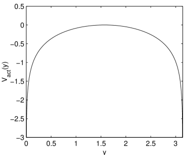
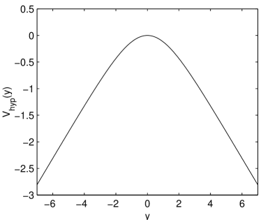
Figure 8: Left: Potential $V(y)$ in the actual genetic drift system. Right: Potential $V(y)$ in the hypothetical system described in the text.

Appendix B Coordinate system in which the Kolmogorov equation is separable

The transformation from the coordinate system defined in terms of the set of allele frequencies, $x_{i}$, to that denoted by $u_{i}$, for which the Kolmogorov equation is separable, is given by Eq. (10), with the inverse transformation given by Eq. (11). In this Appendix we explore the nature of this transformation, determine the Jacobian of the transformation and calculate how the jump moments in the new coordinate system are related to those in the old one. This enables us to derive the Kolmogorov equation in the new variables—given by Eqs. (12) and (13) in the main text. We begin by looking at the nature of the transformation for low values of $M$.

$\underline{M=2}$: $0\leq x_{1}\leq 1$.

$u_{1}=x_{1}\ \ \Rightarrow 0\leq u_{1}\leq 1$.

$\underline{M=3}$: $0\leq x_{1},x_{2}\leq 1$. Since $x_{3}=1-x_{1}-x_{2}$ also satisfies this condition, then $x_{1}+x_{2}\leq 1$.

$$u_{1}=x_{1}\,,\ \ \ u_{2}=\frac{x_{2}}{1-x_{1}}\,.$$

Therefore, $0\leq u_{1},u_{2}\leq 1$, with the three lines $x_{1}=0\ (0\leq x_{2}\leq 1)\,,x_{2}=0\ (0\leq x_{1}\leq 1)$ and $x_{1}+x_{2}=1\ (0\leq x_{1}<1)$ go over to the three lines $u_{1}=0\ (0\leq u_{2}\leq 1)\,,u_{2}=0\ (0\leq u_{1}\leq 1)$ and $u_{2}=1\ (0\leq u_{1}<1)$ respectively. The point $x_{1}=1,x_{2}=0$ goes over to the line $u_{1}=1\ (0\leq u_{2}\leq 1)$. This is illustrated in Fig. 9

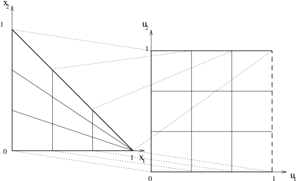
Figure 9: Schematic representation of the mapping of points in the $x_{1}-x_{2}$ plane onto the $u_{1}-u_{2}$ plane.

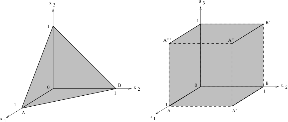
Figure 10: The range of values that can be taken by $x_{i}$ and $u_{i}$ in a 4 allele system. The points $A,A^{\prime},A^{\prime\prime}$ and $A^{\prime\prime\prime}$ on the right all map onto the point $A$ on the left. Similarly, $B$ and $B^{\prime}$ both map onto $B$.

$\underline{M=4}$: $0\leq x_{1},x_{2},x_{3}\leq 1$ with the additional condition $x_{1}+x_{2}+x_{3}\leq 1$.

$$u_{1}=x_{1}\,,\ \ \ u_{2}=\frac{x_{2}}{1-x_{1}}\,,\ \ \ u_{3}=\frac{x_{3}}{1-x_{1}-x_{2}}\,.$$

Therefore, $0\leq u_{1},u_{2},u_{3}\leq 1$. The planes $x_{i}=0$ get mapped on to the planes $u_{i}=0$ ($i=1,2,3$), the plane $x_{1}+x_{2}+x_{3}=1,\ x_{1}+x_{2}\neq 1$ gets mapped on to the plane $u_{3}=1,\ 0\leq u_{1},u_{2}<1$, the line $x_{1}+x_{2}+x_{3}=1,\ x_{1}+x_{2}=1,\ x_{1}\neq 1$ gets mapped to the plane $u_{2}=1,\ 0\leq u_{3}\leq 1,\ 0\leq u_{1}<1$ and the point $x_{1}+x_{2}+x_{3}=1,\ x_{1}+x_{2}=1,\ x_{1}=1$ gets mapped to the plane $u_{1}=1,\ 0\leq u_{2},u_{3}\leq 1$. This is illustrated in Fig. 10.

General $M$: $0\leq x_{1},\ldots,x_{M-1}\leq 1$ with the additional condition $x_{1}+\ldots+x_{M-1}\leq 1$.

From Eqs. (10) and (11) we see that $0\leq u_{i}\leq 1,\ i=1,\ldots,M-1$. The pattern from the $M=3$ and $M=4$ cases should now be clear: the hyperplanes $x_{i}=0$ get mapped on to the hyperplanes $u_{i}=0$ ($i=1,\ldots,M-1$), the hyperplane $x_{1}+\ldots+x_{M-1}=1,\ x_{M-1}\neq 0$, gets mapped on to the hyperplane $u_{M-1}=1,\ 0\leq u_{1},\ldots,u_{M-2}<1,\ \ldots\$, the point $x_{1}=1,\ x_{i}=0,\ i=2,\ldots,M-2$ gets mapped to the hyperplane $u_{1}=1,\ 0\leq u_{i}\leq 1,\ i=2,\ldots,M-2$.

So, in summary, the region $0\leq x_{i}\leq 1$ lying between the origin and the hyperplane $x_{1}+\ldots+x_{M-1}=1$, gets mapped into the unit hypercube $0\leq u_{i}\leq 1$. However, parts of the hyperplane $x_{1}+\ldots+x_{M-1}=1$ of dimensions $M-1,M-2,\ldots,1$ get mapped on to the hyperplanes $u_{i}=1,\ i=1,\ldots,M-1$.

The Jacobian of the transformation from $\underline{u}$ to $\underline{x}$ is easily found if we note from (11) that $\partial x_{i}/\partial u_{j}=0$ if $j>i$. This implies that the Jacobian has zeros if the column label is greater than the row label, and so the determinant is just the product of the diagonal elements. Since the $i$th diagonal element is simply $x_{i}/u_{i}$, we have that

$$\frac{\partial(x_{1},\ldots,x_{M-1})}{\partial(u_{1},\ldots,u_{M-1})}=\frac{x_{1}}{u_{1}}\frac{x_{2}}{u_{2}}\ldots\frac{x_{M-1}}{u_{M-1}}=\left(1-u_{1}\right)^{M-2}\left(1-u_{2}\right)^{M-3}\ldots\left(1-u_{M-2}\right)\;.$$ (1)

As explained in Section 2.2, the pdfs in the $\underline{u}$ variables, denoted by $\mathcal{P}$, are related to those in the $\underline{x}$ variables, denoted by $P$, by a multiplicative factor which is simply the Jacobian:

$$\mathcal{P}(\underline{u},t) = P(\underline{x},t)\,\frac{\partial(x_{1},\ldots,x_{M-1})}{\partial(u_{1},\ldots,u_{M-1})}\,,$$

$$\mathcal{P}(\underline{u},t_{2};\underline{v},t_{1}) = P(\underline{x},t_{2};\underline{y},t_{1})\,\frac{\partial(x_{1},\ldots,x_{M-1})}{\partial(u_{1},\ldots,u_{M-1})}\,\frac{\partial(y_{1},\ldots,y_{M-1})}{\partial(v_{1},\ldots,v_{M-1})}\,,\ \ldots\ \,,$$

from which (14) follows.

The final point which we wish to discuss in this Appendix is the form of the Kolmogorov equation in the new $\underline{u}$ variables. As discussed in Section 3, the easiest way to determine this is to relate the jump moments in the old coordinate system, defined through Eq. (61), and those in the new coordinate system, defined through Eq. (63). To do this, let us begin with the first jump moment:

$$\left\langle\Delta u_{i}(t)\right\rangle_{\underline{u}(t)=\underline{u}} = \int{\rm d}\underline{u}^{\prime}\left(u_{i}^{\prime}-u_{i}\right)\mathcal{P}(\underline{u}^{\prime},t+\Delta t|\underline{u},t)$$

$$= \int{\rm d}\underline{x}^{\prime}\left(f_{i}(\underline{x}^{\prime})-f_{i}(\underline{x})\right)P(\underline{x}^{\prime},t+\Delta t|\underline{x},t)\,,$$

where we have used (14) and where $u_{i}=f_{i}(\underline{x})$ is the transformation (10). Use of Taylor’s theorem then gives

$$\left\langle\Delta u_{i}(t)\right\rangle_{\underline{u}(t)=\underline{u}} = \sum_{j}\left\langle\Delta x_{j}(t)\right\rangle_{\underline{x}(t)=\underline{x}}\,\frac{\partial f_{i}}{\partial x_{j}}$$ (2)

$$+ \frac{1}{2!}\sum_{j}\sum_{k}\left\langle\Delta x_{j}(t)\Delta x_{k}(t)\right\rangle_{\underline{x}(t)=\underline{x}}\,\frac{\partial^{2}f_{i}}{\partial x_{j}\partial x_{k}}+\ldots\,.$$

Since jump moments higher than the second vanish in the limit $\Delta t\to 0$, we find from Eq. (2) that

$$\tilde{\alpha}_{i}(\underline{u})=\sum_{j}\alpha_{j}(\underline{x})\frac{\partial u_{i}}{\partial x_{j}}+\frac{1}{2}\sum_{j}\sum_{k}\alpha_{jk}(\underline{x})\frac{\partial^{2}u_{i}}{\partial x_{j}\partial x_{k}}\,.$$ (3)

Similarly,

$$\tilde{\alpha}_{ij}(\underline{u})=\sum_{k}\sum_{l}\alpha_{kl}(\underline{x})\frac{\partial u_{i}}{\partial x_{k}}\,\frac{\partial u_{j}}{\partial x_{l}}\,.$$ (4)

The results (3) and (4) tell us how the jump moments transform from one coordinate system to another. In our case, we have from Eq. (10)

$$\frac{\partial u_{i}}{\partial x_{j}}=\left\{\begin{array}[]{ll}u^{2}_{i}/x_{i},&\mbox{\ if $j<i$}\\ u_{i}/x_{i},&\mbox{\ if $j=i$}\\ 0,&\mbox{\ if $j>i$\,,}\end{array}\right.$$ (5)

and

$$\frac{\partial^{2}u_{i}}{\partial x_{k}\partial x_{l}}=\left\{\begin{array}[]{ll}2u^{3}_{i}/x_{i}^{2},&\mbox{\ if $k,l<i$}\\ u_{i}^{2}/x_{i}^{2},&\mbox{\ if ($k=i,l<i$) or ($l=i,k<i$)}\\ 0,&\mbox{\ if $k=l=i$}\\ 0,&\mbox{\ if $k>i$ or $l>i$\,.}\end{array}\right.$$ (6)

The key feature of the two results (5) and (6) is that they only depend on $i$, and not on $j,k$ or $l$. This simplifies the summations which appear in (3) and (4). A still fairly tedious calculation shows that the second term on the right-hand side of (3) is zero and that the terms with $i\neq j$ in (4) are also zero. Specifically,

$$\tilde{\alpha}_{i}(\underline{u}) = \sum_{j}\alpha_{j}(\underline{x})\frac{\partial u_{i}}{\partial x_{j}}=\sum_{j}\left.\frac{{\rm d}x_{j}}{{\rm d}t}\right|_{\rm det}\frac{\partial u_{i}}{\partial x_{j}}=\left.\frac{{\rm d}u_{i}}{{\rm d}t}\right|_{\rm det}\,.$$ (7)

$$\tilde{\alpha}_{ij}(\underline{u}) = \left\{\frac{u_{i}(1-u_{i})}{\prod_{k<i}(1-u_{k})}\right\}\delta_{ij}\,.$$ (8)

In this paper the only deterministic mechanism which we will consider will be mutation, described by the differential equation

$$\frac{{\rm d}x_{i}}{{\rm d}t}=\sum_{j\neq i}m_{ij}x_{j}(t)-\sum_{j\neq i}m_{ji}x_{i}(t)\,,$$ (9)

where $m_{ij}$ is the rate of mutation of allele $j$ into allele $i$. From Eqs. (5) and (7)

$$\tilde{\alpha}_{i}=\frac{u_{i}}{x_{i}}\left\{u_{i}\sum_{j<i}\frac{{\rm d}x_{j}}{{\rm d}t}+\frac{{\rm d}x_{i}}{{\rm d}t}\right\}\,.$$ (10)

We will denote the term in the brackets in Eq. (10) by $\tilde{\beta}_{i}(\underline{u})$, so that

$$\tilde{\alpha}_{i}(\underline{u})=\frac{\tilde{\beta}_{i}(\underline{u})}{\prod_{j<i}(1-u_{j})}\,.$$

Using Eqs. (62) and (8), we find the Kolmogorov equation in the new coordinate system to be

$$\frac{\partial\mathcal{P}}{\partial t}=\frac{1}{\prod_{j<i}(1-u_{j})}\,\sum_{i}\left\{-\frac{\partial}{\partial u_{i}}\left[\tilde{\beta}_{i}(\underline{u})\,\mathcal{P}\right]+\frac{1}{2}\frac{\partial^{2}}{\partial u_{i}^{2}}\left[u_{i}(1-u_{i})\,\mathcal{P}\right]\right\}\,.$$ (11)

In Section 3 we prove that the Kolmogorov equation is separable in the $\underline{u}$ coordinate system if $\tilde{\beta}_{i}(\underline{u})$ depends on $u_{i}$ only, and not on the $u_{j},\ j\neq i$. Since $\tilde{\beta}_{i}$ involves a sum over the expression (9), which has itself to be written in terms of the $\underline{u}$ using Eq. (11), it is clear that this will not be the case for general $m_{ij}$. However, if it is assumed that the rate of mutation of the alleles $A_{j}\ (j\neq i)$ to $A_{i}$ occurs at a constant rate $m_{i}$, independent of $j$, then $m_{ij}=m_{i}$ for all $j\neq i$ and (9) becomes

$$\frac{{\rm d}x_{i}}{{\rm d}t}=m_{i}\left(1-x_{i}(t)\right)-\left(\sum^{M}_{j\neq i}m_{j}\right)x_{i}(t)=m_{i}-\left(\sum^{M}_{j=1}m_{j}\right)x_{i}(t)\,.$$ (12)

In this case

$$\tilde{\beta}_{i} = u_{i}\sum^{i-1}_{j=1}m_{j}-Ru_{i}\sum_{j<i}x_{j}+m_{i}-Rx_{i}$$

$$= u_{i}\sum^{i-1}_{j=1}m_{j}+R(x_{i}-u_{i})+m_{i}-Rx_{i}\,,$$

where $R\equiv\sum^{M}_{j=1}m_{j}$ and where we have used Eq. (11). We see that $\tilde{\beta}_{i}(\underline{u})$ only depends on $u_{i}$ and that

$$\tilde{\alpha}_{i}(\underline{u})=\frac{m_{i}-R_{i}u_{i}}{\prod_{j<i}(1-u_{j})}\,,$$ (13)

where $R_{i}\equiv\sum^{M}_{j=i}m_{j}$. This leads to the Kolmogorov equation

$$\frac{\partial\mathcal{P}}{\partial t}=\frac{1}{\prod_{j<i}(1-u_{j})}\,\sum_{i}\left\{\frac{\partial}{\partial u_{i}}\left[\left(R_{i}u_{i}-m_{i}\right)\;\mathcal{P}\right]+\frac{1}{2}\frac{\partial^{2}}{\partial u_{i}^{2}}\left[u_{i}(1-u_{i})\;\mathcal{P}\right]\right\}\,.$$ (14)

This is the content of Eqs. (12) and (13) in the main text.

Appendix C Explicit solution of the second order differential equations

In this Appendix we will provide further details relating to the solution of the equations (71) and (75) subject to the appropriate boundary conditions. Some of the details have already been given in Section 3, in particular how the substitution (78) leads to the hypergeometric equation (81). Consequently, much of this Appendix will be concerned with the hypergeometric functions $F(a,b;c;u)$ which are the solutions of this equation. We will refer to Chapter 15 of the standard handbook by Abramowitz and Stegun [46] for the formulæ that we use, but several appear sufficiently often that it is worth stating them explicitly here:

• If $c-a-b>0$ and $c\neq 0,-1,-2,\ldots$, then

  $$F(a,b;c;1)=\frac{\Gamma(c)\Gamma(c-a-b)}{\Gamma(c-a)\Gamma(c-b)}\,.$$

• $F(a,b;c,u)=(1-u)^{(c-a-b)}F(a^{\prime},b^{\prime};c;u)$ where $a^{\prime}=c-a$ and $b^{\prime}=c-b$. Note that $c-a^{\prime}-b^{\prime}=-(c-a-b)$.

• If $a$ or $b$ is a non-positive integer then the power series for $F(a,b;c;u)$ terminates:

  $$F(-n,\alpha+1+\beta+n;\alpha+1;u)=\frac{\Gamma(n+1)\Gamma(\alpha+1)}{\Gamma(n+\alpha+1)}P^{(\alpha,\beta)}_{n}(1-2u)\,,$$

  where $P^{(\alpha,\beta)}_{n}$ is a Jacobi Polynomial of order $n$.

As we will see, the solution of the hypergeometric differential equation typically proceeds as follows. The general solution to the equation (81) is written out as $f(u)=Af_{1}(u)+Bf_{2}(u)$, where $f_{1}(u)$ and $f_{2}(u)$ are two independent solutions of the equation, and $A$ and $B$ are two arbitrary constants. Examining the general solution in the vicinity of the boundary at $u=0$ rules out one of the solutions, so that, for instance one must take $B=0$ in order to satisfy the boundary condition there. The remaining solution is now examined in the vicinity of the other boundary at $u=1$. If the solution has the form $F(\hat{a},\hat{b};\hat{c};u)$ with $\hat{c}-\hat{a}-\hat{b}>0$ then we may use Result 1 above. If $\hat{c}-\hat{a}-\hat{b}<0$, then we may use Result 2 followed by Result 1. If it is found that either $\hat{a}$ or $\hat{b}$ is a non-positive integer, then Result 3 may be invoked.

We now separately examine the specific equations encountered in the absence and presence of mutations.

C.1 No mutations

The values of the parameters are given in Section 3.3.2, where it is seen from Eq. (83) that $c=2$. One of the solutions of the hypergeometric equation when $c=2$ (suppose it is $f_{2}$) has the following behaviour for small $u$ [46]:

$$f_{2}(u)\sim\frac{1}{(1-a)(1-b)u}\,,\ \ {\rm as}\ u\to 0\,,$$ (1)

and so this solution would not lead to a finite pdf as $u\to 0$—recall from Appendix A that only divergences less strong than $u^{-1/2}$ will be tolerated. Therefore $B=0$. The remaining solution is $f_{1}(u)=F(a,b;2;u)$. From Eq. (83), $2-a-b=-1-2\gamma_{i}$, so if we choose $\gamma_{i}>0$, as described in Section 3.3.2, we may use Result 2 above to show that

$$f_{1}(u)=\left(1-u\right)^{-2\gamma_{i}-1}F(2-a,2-b;2;u)\,.$$

Now $2-(2-a)-(2-b)=a+b-2=2\gamma_{i}+1>0$ and so we may use Result 1 to show that

$$f_{1}(u) \sim \left(1-u\right)^{-2\gamma_{i}-1}\frac{\Gamma(2\gamma_{i}+1)}{\Gamma(a)\Gamma(b)}\,,\ \ {\rm as}\ u\to 1$$

$$\Rightarrow\ \ \psi(u) \sim \left(1-u\right)^{-\gamma_{i}-1}\frac{\Gamma(2\gamma_{i}+1)}{\Gamma(a)\Gamma(b)}\,,\ \ {\rm as}\ u\to 1\,.$$ (2)

We may once again use the result of Appendix A to deduce that this term cannot be present since it is diverging too fast as $u\to 1$ (the analysis of Appendix A can be straightforwardly generalised to cover the equations that are found from separation of the $M$ allele Kolmogorov equation). We therefore require that either $a$ or $b$ equals $-l$, where $l$ is a non-negative integer. Since the hypergeometric function is symmetric in $a$ and $b$ it does not matter which we choose: let $a=-l$. From Result 3 this means that the hypergeometric function is terminating, and more specifically,

$$f_{1}(u)=F(-l,2\gamma_{i}+l+3;2;u)=\frac{1}{l+1}P^{(1,2\gamma_{i}+1)}_{l}(1-2u)\,.$$ (3)

As shown in Section 3.3.2, $\gamma_{i}=L_{i-1}$, if we take $\gamma_{i}>0$, and so up to a constant

$$\psi_{\lambda^{i};\lambda^{(i-1)}}(u)=\left(1-u\right)^{L_{i-1}}P^{(1,2\gamma_{i}+1)}_{l}(1-2u)\,.$$ (4)

We discuss some properties of Jacobi Polynomials below.

Note that if we had made the choice $\gamma_{i}<0$ in Section 3.3.2 (i.e. $\gamma_{i}=-L_{i-1}-1$), then the argument given above would still rule out solution $f_{2}(u)$ using Eq. (1), but we would have found the remaining solution to be $f_{1}(u)=F(a^{\prime},b^{\prime};2;u)$ where $a^{\prime}$ and $b^{\prime}$ are the parameter solutions relevant for the choice $\gamma_{i}<0$ and are related to those for the former $\gamma_{i}>0$ choice by $a^{\prime}=2-a$ and $b^{\prime}=2-b$. This can be easily seen from Eq. (83): if $\gamma_{i}$ is one solution of $\gamma_{i}(\gamma_{i}+1)=2\lambda^{\prime}$, then a second one is $\gamma_{i}^{\prime}=-1-\gamma_{i}$. But then Eq. (83) is unchanged if $\gamma_{i},a$ and $b$ are replaced by $\gamma_{i}^{\prime},a^{\prime}=2-a$ and $b^{\prime}=2-b$. So for the choice $\gamma^{\prime}=-L_{i-1}-1$ we have shown that

$$\psi(u)=\left(1-u\right)^{-L_{i-1}-1}F(2-a,2-b;2;u)\sim\left(1-u\right)^{-\gamma_{i}-1}\frac{\Gamma(2\gamma_{i}+1)}{\Gamma(a)\Gamma(b)}\,,\ \ {\rm as}\ u\to 1\,,$$

where the $\gamma_{i},a$ and $b$ are those for the $\gamma_{i}>0$ choice. This is exactly Eq. (2) and so we again deduce that $a=-l$, where $l$ is a non-negative integer. Using Result 2 we then have that

$$f_{1}(u) = \left(1-u\right)^{2\gamma_{i}+1}F(-l,2L_{i-1}+l+3;2;u)$$

$$\Rightarrow\ \ \psi_{\lambda^{i};\lambda^{(i-1)}}(u) = \left(1-u\right)^{L_{i-1}}P^{(1,2\gamma_{i}+1)}_{l}(1-2u)\,,$$

which is Eq. (4).

The final step in calculating the solutions is to apply the initial conditions to find the appropriate coefficients. We use the appropriate orthogonality relationship (which we shall give below) and use the method described in (66)-(68), and find $w(\underline{u}_{0})$ and $c_{l_{i}}(L_{i})$ as stated in (19) and (23).

C.2 Mutations present

The values of the parameters are given in Section 3, where it is seen from Eq. (82) that $c=2(1-m_{1})$. The nature of the solutions of Eq. (81) depends on whether $c$ is an integer, and if it is, what its value is [46]. The simplest case is if $c$ is not an integer, then the general solution has the form

$$AF(a,b;c;u)+Bu^{1-c}F(a-c+1,b-c+1;2-c;u)\,.$$ (5)

Both of these hypergeometric functions are of the form $F(a,b;c,u)$ with $c-a-b>-1$ and so have power-series expansions near $u=0$ [46]. Substituting the expression (5) into the boundary condition (90) gives $A=0$. The analysis when $c=1$ and $c=0,-1,-2,\ldots$ has to be done separately. One of the solutions has a factor of $\ln u$ in these cases, but it turns out that, while these solutions have a current which does not diverge at $u=0$, the current is non-zero, which is forbidden by the reflecting boundary conditions. Therefore this solution must be absent. It is found that in all cases the implementation of the boundary condition at $u=0$ shows that the required solution is $f(u)=u^{1-c}F(a-c+1,b-c+1;2-c;u)$.

We now note that the conditions which determine the parameters $a$ and $b$ from Eq. (82) can be simplified if we introduce a new parameter $k_{i}$ through $a=1+\gamma_{i}+k_{i}$. Then $b=\gamma_{i}+2-2R_{i}-k_{i}$, where $k_{i}(2R_{i}+k_{i}-1)=2\lambda$. So choosing $\gamma_{1}=-L$, this being one of the solutions of Eq. (93), we have that $c=2(1-m_{1}),\ a=1+k_{1}-L$ and $b=2-2R_{1}-k_{1}-L$ and therefore $f(u)=u^{2m_{1}-1}F(2m_{1}+k_{1}-L,1-R_{2}-k_{1}-L;2m_{1};u)$. Using Result 2 we may write this in an alternative form:

$$f_{1}(u)=u^{2m_{1}-1}\left(1-u\right)^{2(L+R_{2})-1}F(L-k_{1},k_{1}+L+2R_{1}-1;2m_{1};u)\,.$$ (6)

We may now apply the boundary condition that the current vanishes when $u=1$, which leads to Eq. (90). After some algebra we find that this condition implies

$$0 = \lim_{u\to 1}\left\{u^{2m_{1}}(1-u)^{-L}\right\}\left\{-LF(2m_{1}+k_{1}-L,1-R_{2}-k_{1}-L;2m_{1};u)\right.$$

$$+ \left.\frac{(L-k_{1})(2R_{1}+k_{1}+L-1)}{2m_{1}}\,F(2m_{1}+k_{1}-L,1-R_{2}-k_{1}-L;2m_{1}+1;u)\right\}\,.$$

We may now use Result 1 to show that for $L\geq 1$ the term in the second set of curly brackets has a finite limit as $u\to 1$, specifically this term tends to

$$\frac{(2R_{2}+L-1)\Gamma(2m_{1})\Gamma(2R_{2}+2L-1)}{\Gamma(L-k_{1})\Gamma(2R_{1}+k_{1}+L-1)}\,.$$

Thus either $L-k_{1}$ or $2R_{1}+k_{1}+L-1$ must be a non-positive integer if we are to obtain a finite current (let alone a zero-current) as $u\to 1$. The case $L=0$ may be treated separately, since the first term in the bracket, to which Result 1 does not immediately apply is absent. The same result is found. To show that these conditions also imply a zero current, we may substitute $k_{1}=L+l$ or $k_{1}=1-2R_{1}-L-l$ into Eq. (6) and find, when $k_{1}+L+l$ for instance that

$$0 = \lim_{u\to 1}\left\{u^{2m_{1}}(1-u)^{2R_{2}+L-1}\right\}\left\{-LF(-l,2R_{1}+2L-1+l;2m_{1};u)\right.$$ (7)

$$+ \left.(1-u)\,\frac{{\rm d}}{{\rm d}u}\,F(-l,2R_{1}+2L-1+l;2m_{1}+1;u)\right\}\,.$$

Since by Result 3 the two hypergeometric functions are polynomials of order $l$, the right-hand side is indeed zero if $L\geq 1$, and also when $L=0$, since the first term in the second curly bracket of Eq. (7) is absent. Note that if we had made the choice $k_{1}=1-2R_{1}-L-l$ then the hypergeometric functions which would have appeared would have been of the form $F(2R_{1}+l+1+l,-l;2m_{1};u)$, which again are polynomials by Result 3.

Therefore, returning to Eq. (6), we have found that

$$f_{1}(u)=u^{2m_{1}-1}\left(1-u\right)^{2(L+R_{2})-1}F(-l,2(L+R_{1})-1+l;2m_{1};u)\,.$$

Using Result 3 this is, up to a constant,

$$f_{1}(u)=u^{\alpha}(1-u)^{\beta}P^{(\alpha,\beta)}_{l}(1-2u)\,,$$ (8)

where $\alpha=2m_{1}-1$ and $\beta=2(R_{2}+L)-1$. Writing it in terms of the function $\psi$ we have that

$$\psi^{(1)}_{\lambda^{n};\lambda^{n-1}}(u_{1})=u_{1}^{2m_{1}-1}(1-u_{1})^{2R_{2}+L-1}P^{(2m_{1}-1,2R_{2}+2L-1)}_{l}(1-2u_{1})\,.$$ (9)

It is also straightforward to check that if we made the choice $\gamma_{1}=2R_{2}+L-1$, rather than $\gamma_{1}=-L$, then the analysis near $u=0$ would be as before, but then use of Result 2 would then show that the result we obtain was exactly as before (but with $a$ and $b$ interchanged).

In summary, we have shown that $k_{1}=L+l$, where $l$ is a non-negative integer. Thus for $M=2$, when $\gamma_{1}=0\ \Rightarrow\ L=0$, and so from $2\lambda=k_{1}(2R_{1}+k_{1}-1)$, we obtain Eq. (91). For $M=3$, we use Eq. (92), with $L=l_{1}$ and so obtain $\lambda^{(2)}$ given by

$$\lambda^{(2)}=\frac{1}{2}L^{\prime}\left(2R_{1}+L^{\prime}-1\right)\,,$$ (10)

where $L^{\prime}=L+l$, and $l$ is a non-negative integer and where $R_{1}=\sum^{3}_{j=1}m_{j}$. Continuing in this way we find the result given by Eq. (94).

We again use the orthogonality properties of the Jacobi Polynomials as described in (66)-(68) to define $c_{l_{i}}$ in (33).

C.3 Jacobi Polynomials

All the solutions for the pdfs considered in this paper consist of Jacobi Polynomial $P^{(\alpha,\beta)}_{l}(1-2u)$. All properties of these functions that we require are given in Chapter 22 of Abramowitz and Stegun [46], but here we will list the key results that we use.

The first point to note is that the natural variable for these functions is $z\equiv 1-2u$. Thus while $u\in[0,1],\ z\in[-1,1]$. They satisfy the following orthogonality relation in the $u$ variable:

$$(2l+\alpha+\beta+1)\,\frac{\Gamma(l+1)\,\Gamma(l+\alpha+\beta+1)}{\Gamma(l+\alpha+1)\Gamma(l+\beta+1)}\times\\ \int^{1}_{0}{\rm d}u\,u^{\alpha}(1-u)^{\beta}P^{(\alpha,\beta)}_{l}(1-2u)P^{(\alpha,\beta)}_{l^{\prime}}(1-2u)=\delta_{l,l^{\prime}}\,,$$ (11)

where $\alpha,\beta>-1$. In the eigenfunctions calculated when mutations are present, the functions $\psi^{(i)}$ which make up the right eigenfunction $\Phi_{\lambda}$ as defined in Eq. (31), contain the factor $u^{\alpha}(1-u)^{\beta}$ which appears in Eq. (11), as can be seen in Eq. (32). On the other hand the functions $\theta^{(i)}$ which make up the left eigenfunction $\Theta_{\lambda}$ as defined in Eq. (37), do not contain this factor, as can be seen in Eq. (38). The result is that the right and left eigenfunctions satisfy the simple orthogonality relation $\int{\rm d}\underline{u}\,\Theta_{\lambda}(\underline{u})\Phi_{\lambda^{\prime}}(\underline{u})=\delta_{\lambda,\lambda^{\prime}}$.

Secondly, Kimura uses the notation of a $J$ polynomial, which relates to the Jacobi polynomial as follows:

$$J_{n}(\alpha+2,\alpha+1,1-x)=\frac{\Gamma(n+1)\Gamma(\alpha+1)}{\Gamma(n+\alpha+1)}(-1)^{n}P_{n}^{(1,\alpha)}(1-2x)\,.$$ (12)

In the derivation of the fixation probability In Section 2.4.1 we make use of the following relationship between Jacobi and Legendre polynomials which can be found in Ref. [46]:

$$(1-z^{2})P_{l}^{(1,1)}(z)=\frac{2(l+1)}{(l+2)}\left[P_{l}(z)-zP_{l+1}(z)\right]\,,$$ (13)

as well as this identity for Legendre Polynomials, which can be found in Ref. [54]:

$$zP_{l+1}(z)-P_{l}(z)=\frac{(l+2)}{(2l+3)}[P_{l+2}(z)-P_{l}(z)]\;.$$ (14)

References

- [1] R. A. Fisher, The Genetical Theory of Natural Selection, Clarendon Press, Oxford, 1930.
- [2] S. Wright, Evolution in mendelian populations, Genetics 16 (1931) 97–159.
- [3] R. A. Fisher, On the dominance ratio, Proc. Roy. Soc. Edin. 42 (1922) 321–431.
- [4] S. Wright, The differential equation of the distribution of gene frequencies, Proc. Natl. Acad. Sci. USA 31 (1945) 382–389.
- [5] M. Kimura, Stochastic processes and distribution of gene frequencies under natural selection, Cold Spring Harbour Symp. Quant. Biol. 20 (1955) 33–53.
- [6] D. L. Hull, Science as a Process: An Evolutionary Account of the Social and Conceptual Development of Science, University of Chicago Press, Chicago, 1988.
- [7] D. L. Hull, Science and selection: essays on biological evolution and the philosophy of science, Cambridge University Press, Cambridge, 2001.
- [8] W. Croft, The relevance of an evolutionary model to historical linguistics, to be published.
- [9] W. Croft, The darwinization of linguistics, Selection 3 (2002) 75–91.
- [10] G. Baxter, R. A. Blythe, W. Croft, A. J. McKane, Drift model of language change, in preparation.
- [11] J. F. Crow, M. Kimura, An Introduction to Population Genetics, Harper and Row, New York, 1970.
- [12] M. Kimura, Random genetic drift in a tri-allelic locus; exact solution with a continuous model, Biometrics 12 (1956) 57–66.
- [13] M. Kimura, Random genetic drift in multi-allelic locus, Evolution 9 (1955) 419–435.
- [14] M. Kimura, On probability of fixation of mutant genes in a population, Genetics 47 (1962) 713–719.
- [15] M. Kimura, Number of alleles that can be maintained in finite population, Genetics 49 (1964) 725–738.
- [16] M. Kimura, Average number of generations until fixation of a mutant gene in a finite population, Genetics 61 (1969) 763–771.
- [17] M. Kimura, Diffusion-model of intergroup selection, with special reference to evolution of an altruistic character, Proc. Nat. Acad. Sci. US - Biol. Sci. 80 (1983) 6317–6321.
- [18] R. A. Littler, Loss of variability at one locus in a finite population, Math. Biosciences 25 (1975) 151–163.
- [19] R. A. Littler, A. J. Good, Ages, extinction times, and first passage probabilities for a multiallele diffusion model with irreversible mutation, Theoretical Population Biology 13 (1978) 214–225.
- [20] M. Notohara, Eigen-analysis for the Kolmogorov backward equation for the neutral multi-allelic model, Journal of Mathematical Biology 11 (1981) 235–244.
- [21] T. Maruyama, Genetic-variability maintained by mutation and over-dominant selection in finite populations, Genetics 98 (1981) 441–459.
- [22] S. Karlin, General 2-locus selection models - some objectives, results and interpretations, Theoretical Population Biology 7 (1975) 364–398.
- [23] M. W. Feldman, R. C. Lewontin, I. R. Franklin, F. B. Christiansen, Selection in complex genetic systems .3. effect of allele multiplicity with 2 loci, Genetics 79 (1975) 333–347.
- [24] I. R. Franklin, M. W. Feldman, 2 loci with 2 alleles - linkage equilibrium and linkage disequilibrium can be simultaneously stable, Theoretical Population Biology 12 (1977) 95–113.
- [25] R. A. Littler, A. J. Good, Fixation times and probabilities for an independent loci model in genetics, Theoretical Population Biology 14 (1978) 204–214.
- [26] G. B. Golding, C. Strobeck, 2-locus, 4th-order gene-frequency moments - implications for the variance of squared linkage disequilibrium and the variance of homozygosity, Theoretical Population Biology 24 (1983) 173–191.
- [27] R. C. Lewontin, M. W. Feldman, A general asymptotic property of 2-locus selection models, Theoretical Population Biology 34 (1988) 177–193.
- [28] Z. B. Zeng, H. Tachida, C. C. Cockerham, Effects of mutation on selection limits in finite populations with multiple alleles, Genetics 122 (1989) 977–984.
- [29] M. Iizuka, M. Takefu, Average time until fixation of mutants with compensatory fitness interaction, Genes and Genetic Systems 71 (1996) 167–173.
- [30] M. Rattray, J. L. Shapiro, Cumulant dynamics of a population under multiplicative selection, mutation, and drift, Theoretical Population Biology 60 (2001) 17–31.
- [31] Y. Wang, B. Rannala, A novel solution for the time-dependent probability of gene fixation or loss under natural selection, Genetics 168 (2004) 1081–1084.
- [32] J. H. Gillespie, The neutral theory in an infinite population, Gene 261 (2000) 11–18.
- [33] J. R. Pannell, S. C. M. Barrett, Effects of population size and metapopulation dynamics on a mating-system polymorphism, Theoretical Population Biology 59 (2001) 145–155.
- [34] R. K. P. Zia, R. J. Astalos, Statistics of an aged stuructured population with two competing species: analytic and Monte Carlo studies, in: D. P. Landau, S. P. Lewis, H.-B. Schuttler (Eds.), Computer Simulation Studies in Condensed Matter Physics XIV, Springer-Verlag, Berlin, 2002, pp. 235–254.
- [35] J. L. Cherry, J. Wakeley, A diffusion approximation for selection and drift in a subdivided population, Genetics 163 (2003) 421–428.
- [36] J. Roughgarden, Theory of Population Genetics and Evolutionary Ecology, MacMillan, New York, 1979.
- [37] D. L. Hartl, A Primer of Population Genetics, Sinauer Associates, Inc., Sunderland, Mass., 2000.
- [38] M. Kimura, Diffusion Models in Population Genetics, Methuen, London, 1964.
- [39] W. J. Ewens, Mathematical Population Genetics, Springer-Verlag, Berlin, 1979.
- [40] H. Risken, The Fokker-Planck Equation, Springer, Berlin, 1989.
- [41] C. W. Gardiner, Handbook of Stochastic Methods, 3rd Edition, Springer, Berlin, 2004.
- [42] W. Feller, The parabolic differential equations and the associated semigroup of transformations, Annals of Mathematics 55 (1952) 468–519.
- [43] C. Tier, A tri-allelic diffusion model with selection, migration, and mutation, Math. Biosciences 44 (1979) 41–60.
- [44] S. Wright, The distribution of gene frequencies under irreversible mutation, Proc. Natl. Acad. Sci. USA 24 (1938) 253–259.
- [45] M. Kimura, Diffusion models in population genetics with special reference to fixation time of molecular mutants under mutational pressure, in: T. Ohta, K. Aoki (Eds.), Population Genetics and Molecular Evolution, Japan Sci. Soc. Press/Springer-Verlag, 1985, pp. 19–39.
- [46] M. Abramowitz, I. Stegun (Eds.), Handbook of Mathematical Functions, Dover, New York, 1965.
- [47] J. Crow, M. Kimura, Some genetic problems in natural populations, in: J. Neyman (Ed.), Proceedings of the Third Berkeley Symposium on Mathematical Statistics and Probability, Volume 4, University of California Press, Berkeley, 1956, pp. 1–22.
- [48] P. M. Morse, H. Feshbach, Methods of Theoretical Physics, McGraw-Hill, New York, 1953.
- [49] M. Mitchell, An Introduction to Genetic Algorithms, MIT Press, Cambridge, Mass., 1996.
- [50] U. Witt (Ed.), Evolutionary Economics, Edward Elgar, Aldershot, 1993.
- [51] M. H. Christiansen, S. Kirby, Language Evolution, Studies in the Evolution of Language, Oxford University Press, Oxford, 2003.
- [52] W. Feller, Diffusion processes in one dimension, Transactions of the American Mathematical Society 77 (1954) 1–31.
- [53] T. Maruyama, Stochastic Problems in Population Genetics, Springer-Verlag, Berlin, 1977.
- [54] I. Gradshteyn, I. Ryzhik, Tables of Integrals, Series, and Products, 5th Edition, Academic Press, Inc., San Diego, 1994.