Pseudopotential method for higher partial wave scattering

Abstract

We present a zero-range pseudopotential applicable for all partial wave interactions between neutral atoms. For $p$- and $d$-waves we derive effective pseudopotentials, which are useful for problems involving anisotropic external potentials. Finally, we consider two nontrivial applications of the $p$-wave pseudopotential: we solve analytically the problem of two interacting spin-polarized fermions confined in a harmonic trap, and analyze the scattering of $p$-wave interacting particles in a quasi-two-dimensional system.

Modeling of two-body interactions is the basic step in development of theories of many-body systems. In the ultracold regime, atomic collisions are dominated by $s$-wave scattering, and interactions can be accurately modeled by the Fermi-Huang pseudopotential Fermi ; Huang . The situation changes, however, in the presence of scattering resonances, which can strongly enhance the contribution from higher partial waves. Such possibility has been demonstrated in recent experiments by employing Feshbach resonances to tune the interactions of identical fermions in $p$-wave Regal ; Zhang . In this context, the development of pseudopotentials for higher partial wave scattering is of crucial importance for the theoretical description of ultracold gases with $l\neq 0$ interactions.

There are several approaches in the literature to derive pseudopotential valid for all partial waves. The first derivation comes from Huang and Yang Huang . Their pseudopotential, however, is incorrect with respect to $l>0$ waves, as recently shown in Roth . Several alternatives have been proposed Roth ; Stock ; Omont ; Kanjilal ; Pricoupenko , which have specific limitations. For instance, Roth entails no regularization and is only applicable to mean-field theories; Stock requires knowledge of the wave function in the inner region of the shell potential, and taking the limit of shell radius going to zero in the final step of the calculation.

In this Letter we address the problem of interactions in all partial waves. We correct the original derivation of Huang and Yang and obtain a comparatively simple pseudopotential. Next, we derive explicit pseudopotential forms for $p$- and $d$-wave interactions, that are are very convenient in calculations involving anisotropic external potentials. We illustrate this by solving analytically the problem of two identical fermions confined in an anisotropic harmonic trap. We finally turn to interactions of atoms in low dimensional systems. We apply our $p$-wave pseudopotential to analyze the $p$-wave scattering in quasi-two-dimensional (Q2D) system, and show the occurrence of confinement-induced resonances analogous to $s$-wave scattering Olshanii ; Petrov , and $p$-wave scattering in Q1D Granger . Our analysis is of direct interest for studies of controlled interactions between tightly confined fermionic atoms, relevant for applications to quantum information processing.

First, we derive the pseudopotential for interactions in all partial waves. We start from the Schrödinger equation for the relative motion

$$\frac{\hbar^{2}}{2\mu}(\Delta+k^{2})\Psi(\mathbf{r})=V(r)\Psi(\mathbf{r}),$$ (1)

where $k^{2}=2\mu E/\hbar^{2}$, and $\mu$ denotes the reduced mass. We assume that the potential $V(r)$ is central and has a finite range. Outside the range of the potential, the wave function exhibits the following asymptotic behavior

$$\Psi_{a}(\mathbf{r})=\sum_{l=0}^{\infty}\sum_{m=-l}^{l}R_{l}(r)Y_{lm}(\theta,\phi),$$ (2)

where $Y_{lm}(\theta,\phi)$ are spherical harmonics, the radial wave functions $R_{l}=C_{lm}[j_{l}(kr)-\tan\delta_{l}n_{l}(kr)]$ are linear combinations of spherical Bessel and Neumann functions $j_{l}(r)$ and $n_{l}(r)$, $C_{lm}$ are coefficients that depend on the boundary condition for $r\rightarrow\infty$, and the phase shifts $\delta_{l}$ are determined by the potential $V(r)$. Our goal is to replace $V(r)$ by contact potential $V_{ps}(r)$, which acts only at $\mathbf{r}=0$ and gives the same asymptotic function $\Psi_{a}(\mathbf{r})$ as the real potential $V(r)$. Following Huang and Yang Huang , we determine the pseudopotential from $V_{ps}(\mathbf{r})\Psi_{a}(\mathbf{r})=\hbar^{2}/(2\mu)(\Delta+k^{2})\Psi_{a}(\mathbf{r})$. Since $j_{l}(kr)$ is regular at $\mathbf{r}=0$, the only contribution to the pseudopotential comes from the behavior of $n_{l}(kr)$ for small $r$: $n_{l}(x)\sim-(2l-1)!!/x^{l+1}$. Hence

$$V_{ps}(\mathbf{r})\Psi_{a}(\mathbf{r})= \frac{\hbar^{2}}{2\mu}\sum_{l=0}^{\infty}\sum_{m=-l}^{l}(2l-1)!!C_{lm}\tan\delta_{l}Y_{lm}(\theta,\phi)$$

$$\times\!\left[\frac{d^{2}}{dr^{2}}+\frac{2}{r}\frac{d}{dr}-\frac{l(l+1)}{r^{2}}\right]\!\frac{1}{(kr)^{l+1}}.$$ (3)

To calculate the action of the radial part of the Laplace operator on the function $1/r^{l+1}$ at $r=0$, one has to resort to the theory of generalized functions. By applying the Hadamard finite part regularization of the singular function $1/r^{k}$ Kanwal ; Estrada , one can prove the following identity

$$\left[\frac{d^{2}}{dr}+\frac{2}{r}\frac{d}{dr}-\frac{l(l+1)}{r^{2}}\right] \frac{1}{r^{l+1}}=\frac{(-1)^{l+1}(2l+1)}{l!}\frac{\delta^{(l)}(r)}{r^{2}},$$ (4)

where $\delta^{(n)}(r)$ denotes the $n$-th derivative of the delta function. In comparison, Huang and Yang calculate (4) by mapping on $\delta(\mathbf{r})/r^{l}$, which leads them to the incorrect result. In the final step of the derivation we express the coefficients $C_{lm}$ in terms of the regularization operator $\partial_{r}^{2l+1}r^{l+1}$: $C_{lm}=(2l+1)!!/[k^{l}(2l+1)!][\partial_{r}^{2l+1}r^{l+1}R_{l}(r)]_{\mathbf{r}=0}$. In this way we obtain the following form of the pseudopotential:

$$V_{ps}(\mathbf{r})\Psi(\mathbf{r})= \frac{\hbar^{2}}{2\mu}\sum_{l=0}^{\infty}\frac{(-1)^{l+1}\,[(2l+1)!!]^{2}}{4\pi(2l)!\,l!}\frac{\tan\delta_{l}}{k^{2l+1}}\frac{\delta^{(l)}(r)}{r^{2}}$$

$$\times\left[\frac{\partial^{2l+1}}{\partial{r^{\prime}}^{2l+1}}{r^{\prime}}^{l+1}\!\int\!\!d\Omega^{\prime}P_{l}(\mathbf{n}\!\cdot\!\mathbf{n}^{\prime})\Psi(\mathbf{r}^{\prime})\right]_{\mathbf{r}^{\prime}=0},$$ (5)

where the angular integral over $\Omega^{\prime}$ acts as a projection operator on a state with a given quantum number $l$. Here, $P_{l}(x)$ is the Legendre polynomial, $\mathbf{n}=\mathbf{r}/r$, and $\mathbf{n}^{\prime}=\mathbf{r}^{\prime}/r^{\prime}$. We note that in the calculation of the matrix elements of $V_{ps}(\mathbf{r})$ the differentiation of the delta function is equivalent to differentiation of the function that acts on the l.h.s. of the pseudopotential, with a proper change of sign. Moreover, for functions behaving like $r^{l}$ for small $r$, one can substitute $\delta^{(l)}(r)=(-1)^{l}l!\delta(r)/r^{l}$ and $\delta(r)=4\pi r^{2}\delta(\mathbf{r})$ which shows that the $s$-wave component of (5) is equivalent to Fermi-Huang pseudopotential: $-2\pi\hbar^{2}\tan\delta_{0}/(\mu k)\delta(\mathbf{r})$, whereas components with $l>0$ differ from the pseudopotential of Huang and Yang Huang by a prefactor.

Now we derive an alternative form of the pseudopotential, with projection operators expressed in terms of the differential operators. Such representation is particularly useful for problems involving anisotropic external potentials, since in this case the wave function, containing several components of the angular momentum, has to be projected on a given partial wave interaction. Let us first focus on $p$-wave interactions. Expressing radial derivatives in terms of the gradient operator $\partial_{r}=\mathbf{n}\!\cdot\!\bm{\nabla}$, where $\bm{\nabla}=(\partial_{x},\partial_{y},\partial_{z})$, and performing the angular integration in the projection operator, we obtain the following form of the pseudopotential for $p$-wave interactions

$$V_{p}(\mathbf{r})=\frac{\pi\hbar^{2}a_{p}(k)^{3}}{\mu}\stackrel{{\scriptstyle\leftarrow}}{{\nabla}}\delta(\mathbf{r})\stackrel{{\scriptstyle\rightarrow}}{{\nabla}}r\frac{\partial^{3}}{\partial r^{3}}r^{2},$$ (6)

where $a_{p}$ is the $p$-wave scattering length: $a_{p}(k)^{3}=-\tan\delta_{1}(k)/k^{3}$, and the symbol $\stackrel{{\scriptstyle\leftarrow}}{{\nabla}}$ ($\stackrel{{\scriptstyle\rightarrow}}{{\nabla}}$) denotes the gradient operator that acts to the left (right) of the pseudopotential. To derive (6), in the operator acting to the r.h.s. of the pseudopotential, we introduced an additional multiplication by $r$: $\partial^{3}_{r}r^{2}\rightarrow\partial_{r}r\partial^{3}_{r}r^{2}=\mathbf{n}\!\cdot\!\bm{\nabla}r\partial^{3}_{r}r^{2}$, which is equivalent for terms of the order of $r$, giving the contribution to the matrix elements. In this way we preserve the form of the regularization operator, which is crucial for an exact treatment of the interacting atoms. We note that the pseudopotential for $p$-wave interactions in the form containing a scalar product of gradients has been derived for the first time by Omont Omont , however, in Omont it contained an incorrect prefactor, and did not include the regularization operator. We stress that the presence of the full regularization operator $\partial_{r}^{3}r^{2}$ on the r.h.s. of the pseudopotential (6) is important, since for anisotropic external potentials the exact wave functions obtained in the pseudopotential method contains terms behaving like $x_{i}/r$ for small $r$. Such terms, for instance, are not removed by the operator $\bm{\nabla}\partial_{r}^{2}r^{2}$ Kanjilal .

A similar procedure can be repeated for $d$-wave interactions. In this case we obtain the following pseudopotential

$$V_{d}(\mathbf{r})=g_{d}\sum_{i,j,k,l} {D_{ijkl}}\!\!\!\!\!{\phantom{\Big{)}}}^{\leftarrow}\!\!\Big{(}\partial^{2}_{x_{i}x_{j}}\Big{)}\delta(\mathbf{r})\Big{(}\partial^{2}_{x_{k}x_{l}}\Big{)}^{\!\!\rightarrow}r^{2}\!\frac{\partial^{5}}{\partial r^{5}}r^{3},$$ (7)

where $D_{ijkl}=\delta_{ik}\delta_{jl}-\frac{1}{3}\delta_{ij}\delta_{kl}$, $g_{d}=\pi\hbar^{2}a_{d}(k)^{5}/(8\mu)$ and $a_{d}(k)$ is the $d$-wave scattering length: $a_{d}(k)^{5}=-\tan\delta_{2}(k)/k^{5}$. As can be easily verified, the pseudopotential (7) does not give any contribution for functions exhibiting $s$- and $p$-wave symmetries, which results from the implicit projection on $d$-wave contained in (7).

Two interacting spin-polarized fermions in a harmonic trap.— We start from the integral form of the Schrödinger equation for the relative motion of atoms

$$\Psi(\mathbf{r})=\int\!\!d^{3}r^{\prime}\,G(\mathbf{r},\mathbf{r}^{\prime})V_{p}(\mathbf{r}^{\prime})\Psi(\mathbf{r}^{\prime}),$$ (8)

where $G(\mathbf{r},\mathbf{r}^{\prime})=\langle\mathbf{r}|(E-\hat{H})^{-1}|\mathbf{r}^{\prime}\rangle$ is the single-particle Green function, and $\hat{H}$ is the Hamiltonian including the external potential. For a harmonic potential $G(\mathbf{r},\mathbf{r}^{\prime})$ can be represented by the following integral

$$G(\mathbf{r},\mathbf{r}^{\prime})=- \frac{(\eta_{x}\eta_{y}\eta_{z})^{1/2}}{(2\pi)^{3/2}d^{3}\hbar\omega}\ \int_{0}^{\infty}\!\!\!dt\,e^{Et/(\hbar\omega)}$$

$$\times\prod_{k}\frac{\exp\left(\eta_{k}\frac{x_{k}x_{k}^{\prime}-\frac{1}{2}(x_{k}^{2}+x_{k}^{\prime 2})\cosh(t\eta_{k})}{d^{2}\sinh(t\eta_{k})}\right)}{\sinh(\eta_{k}t)^{1/2}},$$ (9)

which is convergent for energies smaller than the energy of zero-point oscillations $E_{0}=\hbar(\omega_{x}+\omega_{y}+\omega_{z})/2$. For $E>E_{0}$ the Green function can be determined by analytic continuation of (Pseudopotential method for higher partial wave scattering). Here, $d=\sqrt{\hbar/(\mu\omega)}$, $\eta_{k}=\omega_{k}/\omega$, $\omega$ denotes some reference frequency, and the product in (Pseudopotential method for higher partial wave scattering) runs over $k=x,y,z$.

Inserting the pseudopotential (6) into (8), we obtain a set of linear equations $\sum_{l}A_{kl}(E)c_{l}=c_{k}$, where the coefficients $c_{l}=\left[\partial_{x_{l}}r\partial_{r}^{3}r^{2}\Psi(\mathbf{r})\right]_{\mathbf{r}=0}$, and the matrix elements are given by $A_{kl}(E)=\pi(a_{p}/d)^{3}[\partial_{x_{k}}r\partial_{r}^{3}r^{2}\partial_{x_{l}^{\prime}}G(\mathbf{r},\mathbf{r}^{\prime})]_{\mathbf{r}=\mathbf{r}^{\prime}=0}$. The energy levels are determined from the secular equation of the matrix $A(E)-I$. Below we discuss the case of axially symmetric traps: $\omega_{x}=\omega_{y}=\omega_{\perp}=\eta\omega_{z}$. For pancake-shape traps with the anisotropy coefficient $\eta=1/n$ where $n$ is some integer, the equations determining the energy spectrum have the relatively simple form

$$\frac{d_{z}^{3}}{a_{p}^{3}}= -\frac{8}{n}\sum_{k=0}^{n-1}\frac{\Gamma(\frac{k+1/2}{n}-\frac{\cal E}{2}+\frac{3}{4})}{\Gamma(\frac{k+1/2}{n}-\frac{\cal E}{2}-\frac{3}{4})},\quad m=0,$$ (10)

$$\frac{d_{z}^{3}}{a_{p}^{3}}= -\frac{8}{n^{2}}\sum_{k,l=0}^{n-1}\frac{\Gamma(\frac{k+l+1}{n}-\frac{\cal E}{2}+\frac{1}{4})}{\Gamma(\frac{k+l+1}{n}-\frac{\cal E}{2}-\frac{5}{4})},\quad m=\pm 1,$$ (11)

where ${\cal E}=E/(\hbar\omega_{z})$, $d_{z}=\sqrt{\hbar/(\mu\omega_{z})}$ and $m$ is the projection of the angular momentum on the $z$-axis. As it can be easily verified, for the case of spherically symmetric trap ($\eta=1$), Eqs. (10)-(11) coincide with the result of Refs. Stock ; Kanjilal . We note that in the presence of an anisotropic the degeneracy between states with $m=0$ and $m=\pm 1$ is lifted. We have derived similar closed analytic formulas for cigar-shape traps with $\eta=n$ IdziaszekPrep , however, we do not present them in the present letter because of their rather complicated form. In general, when $\eta\neq 1/n$ and $\eta\neq n$, the energy levels can be determined from an implicit equation involving the integral representation (Pseudopotential method for higher partial wave scattering) .

Figs. 1(a) and 1(b) show the energy levels in harmonic traps with $\eta=1/10$ and $\eta=10$, for different values of the quantum number $m$. We observe that for small and positive values of the scattering volume, the system does not have eigenstates with energies smaller than the lowest eigenenergy for noninteracting atoms, This particular behavior results from the properties of the $p$-wave pseudopotential. In this regime of energies, however, it is necessary to include in the calculation the energy-dependence of the pseudopotential. To this end it is sufficient to insert in the pseudopotential (6) the energy dependence of the phase-shift $\delta_{1}(k)$, and calculate the energy spectrum in a self-consistent way. This extends the applicability of the pseudopotential method to the large scattering lengths and tight confining potentials and allows to describe the entire molecular spectrum of the realistic potential Bolda ; Stock .

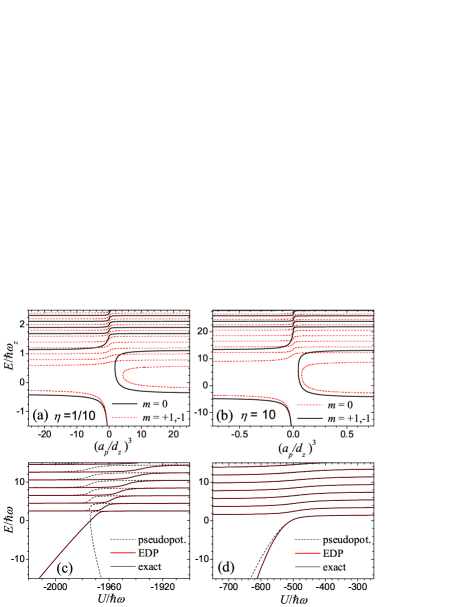
Figure 1: (a)-(b): Energy spectrum of the two fermions interacting in $p$-wave as a function of the scattering volume $a_{p}^{3}/d^{3}$, with $d=\sqrt{\hbar/\mu\omega_{z}}$. The two particles are confined in an axially symmetric harmonic trap with $\eta=\omega_{\perp}/\omega_{z}=0.1$ (a), and $\eta=10$ (b). (c)-(d) Energy spectrum of two atoms interacting via a square-well model potential as a function of the well depth $U$. The atoms are confined in an isotropic harmonic potential and interact in $p$-wave (c) and $s$-wave (d).

To illustrate this procedure we calculate the energy spectrum for a square-well model interaction, assuming for simplicity spherically symmetric harmonic trap. Fig. 1(c) presents the energy levels of $p$-wave interacting particles as a function of the square-well depth $U$ calculated for the square-well radius $R_{0}=0.05d$. The depth $U$ is varied close to the resonance scattering for $p$-wave, related to the appearance of a bound state at $U=-1974\hbar\omega$. The exact energy levels are compared with predictions of the pseudopotential method given by Eq. (10), and with the energy spectrum calculated in a self-consistent way from Eq. (10) with $a_{p}^{3}$ replaced by $a_{p}(k)^{3}=-\tan\delta_{1}(k)/k^{3}$. For comparison, Fig. 1(d) shows the energy levels of $s$-wave interacting atoms, given in the pseudopotential approximation by $d/a_{s}=2\Gamma(\frac{3}{4}-\frac{\cal E}{2})/\Gamma(\frac{1}{4}-\frac{\cal E}{2})$ Busch , where ${\cal E}=E/(\hbar\omega)$ and $a_{s}$ is the $s$-wave scattering length.

One observes that self-consistent calculation with energy-dependent pseudopotential (EDP) provides very accurate results for the energy spectrum. On the other hand, the ordinary pseudopotential method fails for large scattering volumes, and for energies where the bound state of the square well potential appears. Moreover, its range of applicability decreases for higher energy levels. For comparison, the ordinary $s$-wave pseudopotential is incorrect only with respect to deep bound-states.

This behavior can be explained by analyzing the effective range expansion: $k^{3}\cot\delta_{1}(k)=-1/a_{p}^{3}-k^{2}/(2R^{\ast})+{\cal O}(k^{4})$, where $R^{\ast}$ can be interpreted as effective range for $p$-wave (for square-well $R^{\ast}=R_{0}/3$). The second term in the expansion can be neglected when $k|a_{p}|\ll(kR^{\ast})^{1/3}$, which combined with the condition for the applicability of the pseudopotential: $kR^{\ast}\ll 1$, gives $k|a_{p}|\ll 1$. Therefore, the regime where one can apply the ordinary, energy-independent pseudopotential for $p$-waves is quite narrow. This can be compared to the $s$-wave, where the analogous condition takes form $k|a|\ll(k\tilde{R})^{-1}$, where $\tilde{R}$ is the effective range for $s$-wave scattering and $(k\tilde{R})^{-1}$ is large.

Scattering of spin-polarized fermions in Q2D systems.— The scattering solution can be found from the Lippmann-Schwinger equation:

$$\Psi(\mathbf{r})=\Psi_{0}(\mathbf{r})+\int\!\!d^{3}r^{\prime}\,G_{+}(\mathbf{r},\mathbf{r}^{\prime})V_{p}(\mathbf{r}^{\prime})\Psi(\mathbf{r}^{\prime}),$$ (12)

where $\Psi_{0}(\mathbf{r})$ represent the wave function of the incoming particle and $G_{+}(\mathbf{r},\mathbf{r}^{\prime})=\langle\mathbf{r}|(E-\hat{H}+i\epsilon)^{-1}|\mathbf{r}^{\prime}\rangle$. The Green function $G_{+}(\mathbf{r},\mathbf{r}^{\prime})$ describing the propagation of outgoing waves, can be determined from Eq.(Pseudopotential method for higher partial wave scattering) by taking the limit $\omega_{\perp}\rightarrow 0$ and performing the analytic continuation for energies $E>E_{0}$.

In 2D the scattered wave in the asymptotic regime ($\rho\rightarrow\infty$) is described by $f(\phi)e^{ik\rho}/\sqrt{\rho}$ with the scattering amplitude $f(\phi)=(2\pi ik)^{-1/2}\sum_{m=-\infty}^{\infty}e^{im\phi}(e^{i2\delta_{m}}-1)$, where $\delta_{m}$ are scattering phase-shifts LL . In the regime of energies $\hbar\omega_{z}/2<E<3\hbar\omega_{z}/2$ the motion in the $z$ direction is frozen and sufficiently far from the scattering center it is described by the ground-state wave function of the harmonic oscillator: $\psi_{0}(z)=e^{-z^{2}/(2d_{z}^{2})}/\pi^{1/4}$. By solving Eq. (12) with the pseudopotential (6), we obtain the scattering solution, which for $p$-wave interactions contains only $m=\pm 1$ scattering waves

$$\Psi(\bm{\rho})\stackrel{{\scriptstyle\rho\rightarrow\infty}}{{\sim}}\psi_{0}(z)\left\{e^{i\mathbf{k}\bm{\rho}}-\frac{4\cos\phi}{1+i\cot\delta_{1}}\frac{e^{ik\rho}}{\sqrt{2\pi ik\rho}}\right\}.$$ (13)

Figure 2: Two-dimensional differential cross section in forward direction $|f(0)|^{2}$ in the scattering of two fermions in a quasi-2D system as a function of $p$-wave scattering volume $a_{p}^{3}$, for different relative energies $E$ of the particles. The inset shows the value of the critical volume $V_{c}$, at which the system exhibits the confinement-induced resonance.

The scattering phase shift $\delta_{1}$ is given by

$$\cot\delta_{1}=-\frac{2}{3\pi k^{2}d_{z}^{2}}\left[\frac{\sqrt{\pi}d_{z}^{3}}{a_{p}^{3}}-{\cal W}\left(\frac{\cal E}{2}-\frac{1}{4}\right)\right],$$ (14)

where ${\cal W}(x)$ is a function taking values of the order of one , and ${\cal E}=E/(\hbar\omega_{z})$. When $\cot\delta_{1}=0$, the system exhibits confinement-induced resonance, which occurs at the scattering volume $V_{c}({\cal E})=\sqrt{\pi}d_{z}^{3}/{\cal W}({\cal E}/2-1/4)$. At low energies (${\cal E}\rightarrow\frac{1}{2}$) function ${\cal W}(x)$ has a well defined limit: ${\cal W}(0)\approx 0.325$, and $V_{c}(0)\approx 5.4d_{z}^{3}$. This qualitatively differs from $s$-wave interactions, where $\cot\delta_{0}$ exhibits logarithmic behavior for small $k$ Petrov and the resonance condition for $k\rightarrow 0$ depends on the relative kinetic energy of the scattered particles. Fig. 2 shows the dependence of the differential cross section $|f(\phi)|^{2}$ at $\phi=0$ on the scattering volume $a_{p}^{3}$ for different values of the energy. We observe that at low energies of the scattered particles the curve is strongly peaked around $V_{c}$. For higher energies the resonance is broader and finally for ${\cal E}\approx 0.525$ disappears. In this regime of energies the resonance is present for positive values of the scattering volume, which can be observed in the inset of Fig. 2 presenting $V_{c}({\cal E})$.

In summary, we presented the zero-range pseudopotential applicable for all partial wave interactions. For $p$- and $d$-waves we derived an alternative representation of the pseudopotential, in which the projection on spherical harmonics is replaced by an appropriate differential operator. The $p$-wave pseudopotential has been applied to calculate analytically the spectrum of two interacting fermions in a harmonic trap, and to study the scattering of identical fermions in a quasi-two-dimensional system.

After completing this paper we learned of recent work of Derevianko Derevianko in which the pseudopotential equivalent to (5) is derived.

We thank L.P. Pitaevskii, R. Stock, and G.V. Shlyapnikov for valuable discussions. T. Calarco acknowledges support from the EC through contract No. IST-2001-38863.

References

• (1) E. Fermi, Ricerca Sci. 7, 12 (1936);
• (2) K. Huang, C.N. Yang, Phys. Rev. 105, 767 (1957); K. Huang, Statistical Mechanics (John Willey & Sons, New York, 1963).
• (3) C.A. Regal, C. Ticknor, J.L. Bohn, D.S. Jin, Phys. Rev. Lett. 90, 053201 (2003).
• (4) J. Zhang et al., Phys. Rev. A. 70, 030702(R) (2004).
• (5) R. Roth, H. Feldmeier, Phys. Rev. A 64, 043603 (2001).
• (6) R. Stock, A. Silberfarb, E.L. Bolda, I.H. Deutsch, Phys. Rev. Lett. 94 023202 (2005).
• (7) A. Omont, J. Phys. (France) 38, 1343 (1977).
• (8) K. Kanjilal and D. Blume, Phys. Rev. A 70, 042709 (2004).
• (9) L. Pricoupenko, cond-mat/0505048.
• (10) M. Olshanii, Phys. Rev. Lett. 81, 938 (1998).
• (11) D.S. Petrov, M. Holzmann, and G.V. Shlyapnikov, Phys. Rev. Lett 84, 2551 (2000).
• (12) B.E. Granger, D. Blume, Phys. Rev. Lett. 92, 133202 (2004).
• (13) R.P. Kanwal, Generalized Functions, Theory and Technique (Academic Press, New York, 1983).
• (14) R. Estrada, R.P. Kanwal, J. Math. Anal. and Appl. 141, 195 (1989).
• (15) Z. Idziaszek, T. Calarco, in preparation.
• (16) Z. Idziaszek, T. Calarco, Phys. Rev. A 71, 050701(R) (2005).
• (17) E.L. Bolda, E. Tiesinga, and P.S. Julienne, Phys. Rev. A 66, 013403 (2002); D. Blume and C.H. Greene, Phys. Rev. A 65, 043613 (2002).
• (18) T. Busch, B.-G. Englert, K. RzaΜ§ΕΌewski, and M. Wilkens, Found. Phys. 28, 549 (1998).
• (19) L.D. Landau, E.M. Lifshitz, Quantum Mechanics (Butterworth-Heinemann, Oxford, 1999).
• (20) A. Derevianko, cond-mat/0507209.