Mean-field dynamics of a Bose-Einstein condensate in a time-dependent triple-well trap: Nonlinear eigenstates, Landau-Zener models and STIRAP

Abstract

We investigate the dynamics of a Bose–Einstein condensate (BEC) in a triple-well trap in a three-level approximation. The inter-atomic interactions are taken into account in a mean-field approximation (Gross-Pitaevskii equation), leading to a nonlinear three-level model. New eigenstates emerge due to the nonlinearity, depending on the system parameters. Adiabaticity breaks down if such a nonlinear eigenstate disappears when the parameters are varied. The dynamical implications of this loss of adiabaticity are analyzed for two important special cases: A three level Landau-Zener model and the STIRAP scheme. We discuss the emergence of looped levels for an equal-slope Landau-Zener model. The Zener tunneling probability does not tend to zero in the adiabatic limit and shows pronounced oscillations as a function of the velocity of the parameter variation. Furthermore we generalize the STIRAP scheme for adiabatic coherent population transfer between atomic states to the nonlinear case. It is shown that STIRAP breaks down if the nonlinearity exceeds the detuning.

I Introduction

The experimental progress in controlling Bose-Einstein condensates (BECs) has led to a variety of spectacular results in the last few years. At very low temperatures, the dynamics of a BEC can be described in a mean-field approximation by the Gross-Pitaevskii (GPE) or nonlinear Schrödinger equation (NLSE) Pita03 . Previously, several authors investigated the dynamics of the NLSE for a double-well potential in a two-mode approximation Smer97 ; Milb97 ; Zoba00 ; Wu00 ; Holt01b ; Dago02 ; Wu03 ; 05catastrophe . Novel features were found, e.g. the emergence of new nonlinear stationary states Dago02 and a variety of new crossing scenarios (cf. 05catastrophe and references therein). Studies of the quantum dynamics beyond mean-field theory were reported in Smer97 ; Holt01b ; Vard01 . First approaches of the coherent control of BECs in driven double-well potentials have been reported Holt01b . Another relevant application of the two-level NLSE is the dynamics of a BEC in an accelerated or tilted optical lattice Wu00 ; Wu03 . Furthermore, the NLSE describes the propagation of light pulses in nonlinear media Dodd82 and its two-level analogon has been studied in the context of a nonlinear optical directional coupler Chef96 . This equation is also known as the discrete self-trapping equation and has been applied, e.g., to the dynamics of quantum dimers. In fact, the characteristic loop structures Wu00 important in the following, have been already observed in this context Esse95 .

In the present paper we will extend these studies to nonlinear three-level quantum systems with special respect to the breakdown of adiabatic evolution due to the nonlinearity. In fact, we investigate the dynamics of a BEC in a three-level system

$$\psi(t)=a(t)\psi_{1}+b(t)\psi_{2}+c(t)\psi_{3}$$ (1)

in a mean-field approach. The dynamics of the coefficients is described by the discrete NLSE

$$H(|a|^{2},|b|^{2},|c|^{2})\left(\begin{array}[]{c}a\\ b\\ c\end{array}\right)={\rm i}\hbar\frac{{\rm d}}{{\rm d}t}\left(\begin{array}[]{c}a\\ b\\ c\end{array}\right)$$ (2)

with the nonlinear three-level Hamiltonian

$$H(|a|^{2},|b|^{2},|c|^{2})=\left(\begin{array}[]{c c c}\epsilon+g|a|^{2}&v&0\\ v&g|b|^{2}&w\\ 0&w&\delta+g|c|^{2}\\ \end{array}\right)\,.$$ (3)

The dynamics preserves the normalization, which is fixed as $|a|^{2}+|b|^{2}+|c|^{2}=1$. Throughout this paper units are rescaled such that all properties become dimensionless and $\hbar=1$.

An experimental setup leading very naturally to the Hamiltonian (3) is the dynamics of a BEC in a triple-well potential. In this case the basis states $\psi_{n}(x)$ are localized in the three wells. Then $\epsilon$ and $\delta$ are the on-site energies of the outer wells and $v$ and $w$ denote the tunneling matrix elements between the wells. These parameters can be varied by controlling the depth or the separation of the wells. The energy scale is chosen such that the on-site energy of the middle well is zero. This situation is illustrated in figure 1.

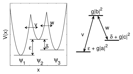
Figure 1: Illustration of the triple-well potential and the corresponding three-level model (3) investigated in the present paper.

A detailed discussion of these approximations and the validity of the model can be found in Milb97 for the case of a double-well potential. Furthermore, the existence of a dark state for ultracold atoms and molecules, which was demonstrated experimentally very recently, could be described successfully within a nonlinear three-level model (see Wink05 and references therein) Further applications include the dynamics of three-mode systems of nonlinear optics or the analysis of the excitonic-vibronic coupled quantum trimer.

As previously shown for the two-level system, the nonlinearity leads to the emergence of new eigenstates without a linear counterpart, loop structures and novel level crossing scenarios. The concept of adiabaticity is very different in the nonlinear case Liu03 , leading to nonlinear Zener tunneling Wu00 and possibly to dynamical instability 05catastrophe . These issues are discussed in section III for the three-level system (3). Furthermore we analyze adiabatic coherent population transfer. In the linear case a complete population transfer can be achieved using the Stimulated Raman Adiabatic Passage (STIRAP) via a dark state of the system Berg98b . Coherent control techniques for ultracold atoms in a triple-well trap were previously investigated by Eckert et. al. for the case of single atoms Ecke04 . In the present paper it is shown that a mean-field interaction plays a crucial role and that the STIRAP scheme fails if the nonlinearity exceeds a critical value due to the breakdown of adiabaticity.

II Nonlinear Eigenstates

Nonlinear eigenstates and eigenvalues can be defined as the solutions of the time-independent NLSE

$$H(|a|^{2},|b|^{2},|c|^{2})\left(\begin{array}[]{c}a\\ b\\ c\end{array}\right)=\mu\left(\begin{array}[]{c}a\\ b\\ c\end{array}\right)$$ (4)

with the chemical potential $\mu$. Obviously an interpretation in terms of linear algebra is not feasible anymore. Therefore – although equation (4) looks like a common eigenvalue-equation – most of the implications of linear quantum mechanics are not valid anymore. Nevertheless these eigenstates are of great importance for understanding the dynamics of the system, as they still are stationary solutions of the time dependent NLSE (2).

In the two-level case one can calculate the eigenstates by solving a forth-order polynomial equation Wu00 . The case of three levels turns out to be a bit more complicated. As all parameters are real, the amplitudes $(a,b,c)$ are also real. For almost all parameters (except in the ”uncoupling” limits $v,w\rightarrow 0$ or $\delta,\epsilon\rightarrow\infty$) the amplitudes are all non-zero. Thus the variables $x=b/a$ and $y=c/b$ are well defined and determined by the equations

$$(1-x^{2}y^{2})\left(g+\delta+\epsilon+v(x+x^{-1})+w(y+y^{-1})\right)$$

$$\quad-3x^{2}+y^{2}(\epsilon+vx)-3wy^{-1}+3\delta=0$$ (5)

$$(1-x^{2})\left(g+\delta+\epsilon+v(x+x^{-1})+w(y+y^{-1})\right)$$

$$\quad-3x^{-1}-3wy+3x^{2}(\epsilon+vx)=0.$$ (6)

Equation (6) can be solved for $y$ explicitly. Substitution of the result into equation (5) then leads to a single equation for $x$, which can be solved numerically. In the limit of large $\delta$ and $\epsilon$, the eigenvalues are easily found by nonlinear optimization with the linear eigenvalues as initial guesses.

Similar to the case of two levels Smer97 , the nonlinear three-level model can also be described as a classical Hamiltonian system. Introducing the variables $p_{1}=|a|^{2}$, $p_{3}=|c|^{2}$, $q_{1}=\arg(b)-\arg(a)$ and $q_{3}=\arg(b)-\arg(c)$, the dynamics is given by the conjugate equations

$$\dot{p}_{j}=-\frac{\partial\cal H}{\partial q_{j}}\quad\mbox{and}\quad\dot{q}_{j}=\frac{\partial\cal H}{\partial p_{j}}$$ (7)

with the classical Hamiltonian function

$${\cal H} \!\!\!\!=\epsilon p_{1}+\delta p_{3}+\dfrac{g}{2}\left(p_{1}^{2}+p_{3}^{2}+(1-p_{1}-p_{3})^{2}\right)$$

$$+2\sqrt{1-p_{1}-p_{3}}\left(v\sqrt{p_{1}}\cos(q_{1})+w\sqrt{p_{3}}\cos(q_{3})\right)$$

and the normalization condition $|b|^{2}=1-|a|^{2}-|c|^{2}$. The eigenstates (4), resp. the stationary states of the system, are given by $\dot{q}_{j}=\dot{p}_{j}=0$. Hence they correspond to the critical points of this classical Hamiltonian, which one finds to be given by the real roots of two polynomials in $p_{1}$ and $p_{3}$, one of them of 8th order in $p_{1}$ and of 7th in $p_{3}$ the other one the opposite way round. At these critical points, the classical Hamiltonian and the chemical potential $\mu$ are simply related by

$${\cal H}=\mu-\dfrac{g}{2}\left(p_{1}^{2}+p_{3}^{2}+(1-p_{1}-p_{3})^{2}\right).$$ (9)

New eigenstates emerge when the nonlinearity $|g|$ is increased, starting from three eigenstates in the linear case $g=0$. From the point of view of standard quantum mechanics, the existence of additional eigenstates is a strange issue. Simply considering them as stationary states is a more adequate point of view. One can intuitively understand that a strong interaction compared to the on-site-energies not only modifies the stationary states of the linear case but can stabilize other states as well and thus create additional eigenstates. For a deeper insight in the features of these states see, e.g., Dago02 , where the nonlinear eigenstates in a symmetric double-well trap are studied in detail.

In terms of the corresponding Hamiltonian system no conflict arises at all. The (dis)appearance of critical points due to a variation of the system parameters is a well-known issue in the theory of classical dynamical systems. In fact this is a major ingredient of catastrophe theory Post78 . Another important results from the theory of classical dynamical systems is that the number of extrema minus the number of saddle points of ${\cal H}$ is constant (see, e.g. Arno80 ) Thus two fixed points, one elliptic and one hyperbolic, always emerge together.

Furthermore this classical description is especially suited for the discussion of adiabatic processes Liu03 . Note that the dynamics of the discrete nonlinear Schrödinger equation can become classically chaotic Thom03 .

III Landau-Zener tunneling

In this section we study the evolution of the system under variation of the parameters in the manner of the Landau-Zener model, considering $v$ and $w$ independent of time. In particular we will focus on the so called equal-slope case Brun93 , for which $\delta$ is constant in time as well and $\epsilon=\alpha t$. In the linear case $g=0$ the instantaneous eigenvalues in dependence of $\epsilon=\alpha t$ (the so called adiabatic levels) form two consecutive avoided crossings which appear at $\epsilon=\lambda_{\pm}$ with gaps of size $v_{1,2}=-{\lambda_{1,2}v}/{n_{2,1}}$ with $\lambda_{1,2}=\delta/2\pm\sqrt{\delta^{2}/4+w^{2}}$ and $n_{1,2}=\sqrt{\lambda_{2,1}^{2}+w^{2}}$. An example is shown in figure 2 (dashed lines). If the system is prepared in a state on the lowest branch for $t\rightarrow-\infty$ and the parameters are varied infinitely slow (i.e. $\alpha\rightarrow 0$) with $g=0$, the adiabatic theorem states that the quantum state will follow the adiabatic eigenstate up to a global phase Mess99 . However, for a finite value of $\alpha$, parts of the population will tunnel to the other adiabatic levels, mainly at the avoided crossings. In the case of the linear two-level system the transition probability $P$ between the two adiabatic levels is given by the celebrated Landau-Zener formula Zene34

$$P_{LZ}=\exp{\left(-{2\pi v^{2}}/{\alpha}\right)}\,.$$ (10)

For the equal-slope case in linear three-level systems, one can show that the transition probability to the highest adiabatic eigenstate (or equivalently the survival probability in the diabatic eigenstate populated initially) is also given by the Landau-Zener-formula (10) and consequently independent of $w$ and $\delta$ (see Demk66 ; Demk68 ; Brun93 and references therein).

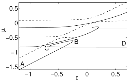
Figure 2: Nonlinear eigenvalues as defined by equation (4) in dependence of $\epsilon$ for $\delta=-0.4$, $v=0.1$, $w=0.2$ and $g=-0.4$ (solid line) resp. $g=0$ (dashed line).

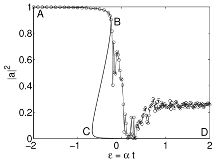
Figure 3: Time evolution of the population in the first level ($|a(t)|^{2}$, open circles $\circ-$) in comparison with the first component of the corresponding adiabatic eigenstates ($|a_{\rm ad}|^{2}$, solid line) for $\epsilon=\alpha t$ with $\alpha=0.001$ and $\delta=-0.4$, $v=0.1$, $w=0.2$ and $g=-0.4$.

In the following we study the behavior of the system in the equivalent scenario with ${g}\neq{0}$. For that purpose we first calculate the nonlinear eigenvalues, which are defined by equation (4). As in the two-level case Wu00 , loops emerge with increasing nonlinearity near the points of the avoided crossings at critical values of $|g|=g_{c1}$ resp. $|g|=g_{c2}$, which are governed by the width of the gap at the avoided crossings in the linear case. An estimate of the critical values $g_{c1}$ and $g_{c2}$ is obtained by considering the two avoided crossings as independent and hence neglecting the influence of the remaining third level. For a two-level system, the critical nonlinearity can be calculated exactly Wu00 , which yields $g_{c1}=2v_{1}$ and $g_{c2}=2v_{2}$. Our numerical studies show that this is an acceptable approximation and at least a lower bound to the real value. An example of the nonlinear eigenvalues in dependence of $\epsilon$ is shown in figure 2 for $\delta=-0.4$, $v=0.1$ and $w=0.2$. We choose $g=-0.4<0$ such that the loops emerge on top of the two lower adiabatic levels for better comparison with Wu00 . However, similar results are found if the signs of both $g$ and $\alpha$ are altered.

The first component of the nonlinear eigenstates associated to the lowest level in figure 2 are illustrated in figure 3 (solid line). The loop structure of the eigenvalues manifests in an S-shaped structure of the components of the corresponding eigenstate Zoba00 . For a better comparison between the figures 2 and 3 we included the labels A-D. The nonlinear eigenstates emerge/vanish in a bifurcation at edges of the loops resp. the S-structure (marked by B and C in the figures).

As in the two-level system, the appearance of the loops leads to the breakdown of adiabatic evolution. To illustrate this issue we calculate the dynamics for the same parameters as above with a slowly varying $\epsilon=\alpha t$ with $\alpha=0.001$ and compare them to the relevant instantaneous eigenstates. The system is initially ($t\rightarrow-\infty$) prepared in an eigenstate corresponding to the lowest level in figure 2 (point A). The resulting dynamics of the population in the first level $|a(t)|^{2}$ is shown in figure 3 (open circles). The solid line shows the population in the first well $|a_{\rm ad}|^{2}$ for the corresponding instantaneous eigenstates. One clearly observes the breakdown of the adiabatic evolution when the adiabatic eigenstate vanishes in a bifurcation at the edge of the S-structure at the point B around $\alpha t\approx-0.25$.

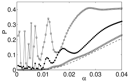
Figure 4: Tunneling probability $P(\alpha)$ in dependence of the velocity of the parameter variation for $g=-0.03$ (open circles), $g=-0.16$ (full circles) and $g=-0.4$ (open squares) and $\delta=-0.4$, $v=0.1$, $w=0.2$. The solid lines are drawn to guide the eye. The Landau-Zener formula (10) for the linear case is shown for comparison (dashed line).

Due to this breakdown of adiabaticity the transition probability $P$ does not vanish for $\alpha\rightarrow 0$ for $|g|>g_{c}$. This is illustrated in fig. 4, where we plotted $P$ in dependence of $\alpha$ for different values of the nonlinear parameter $g$. For weak nonlinearities, e.g. $g=-0.03$ in the figure, $P$ is increased in comparison to the linear case, however it still tends to zero in the adiabatic limit, i.e. $P\rightarrow 0$ for $\alpha\rightarrow 0$, as no loops have occurred yet. This is no longer true after the appearance of the two loops shown in fig. 2 such that $P(\alpha\rightarrow 0)>0$ (cf. fig. 4). These features are well-known from the nonlinear two-level model Wu00 . However, a novel feature is the appearance of pronounced oscillations of the transition probability $P(\alpha)$ for small values of $\alpha$ due to the nonlinear interaction between the different levels.

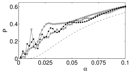
Figure 5: Tunneling probability $P(\alpha)$ in dependence of the velocity of the parameter variation for $w=0.2$ (open circles), $w=0.4$ (full circles) and $w=0.6$ (open squares) and $\delta=-0.4$, $v=0.1$ and $g=-0.4$. The solid lines are drawn to guide the eye. The Landau-Zener formula (10) for the linear case is shown for comparison (dashed line).

As mentioned above, the transition probability for the linear case is independent of $w$ and $\delta$. This does not hold in the nonlinear case any longer, since the influence of the nonlinearity, e.g. the emergence and the structure of the loops, obviously depends on $v,\,w$ and $\delta$. This is confirmed by our numerical results shown in fig. 5, where $P(\alpha)$ is plotted for different values of $w$. Again pronounced oscillations of $P(\alpha)$ are found for small values of $\alpha$. These oscillations and their dependence on the system’s parameters will be studied in detail in a subsequent paper.

IV Nonlinear STIRAP

The STIRAP method, primarily proposed and realized for atomic three-level systems Berg98b , allows a robust coherent population transfer between quantum states. In the meanwhile STIRAP has been generalized to systems with multiple levels and the preparation of coherent superposition states Vita01 . In this case the coupling between the atomic bare states are realized by slightly detuned time-dependent laser fields with Rabi frequencies $v(t)$ and $w(t)$. In the rotating wave approximation at the two-photon resonance, the dynamics of the three-level atom is given by the Hamiltonian (3) with $g=0$ and a fixed detuning $\Delta=-\delta=-\epsilon$. Using the STIRAP scheme one can achieve a complete population transfer from level $\psi_{1}$ to level $\psi_{3}$ by an adiabatic passage via a dark state $\psi_{\rm ds}$ of the system, which is a superposition of $\psi_{1}$ and $\psi_{3}$ alone. If the coupling $w(t)$ between the levels $\psi_{2}$ and $\psi_{3}$ is turned on before the coupling $v(t)$ between the levels $\psi_{1}$ and $\psi_{2}$, the system’s dark state is rotated from $\psi_{\rm ds}(t=-\infty)=\psi_{1}$ to $\psi_{\rm ds}(t=+\infty))=\psi_{3}$. If the parameters $v(t)$ and $w(t)$ are varied sufficiently slowly, the system can follow the dark state adiabatically which leads to a complete population transfer from level $\psi_{1}$ to $\psi_{3}$. This counterintuitive pulse sequence of the coupling elements $v(t)$ and $w(t)$ is illustrated in fig. 6 (upper panel).

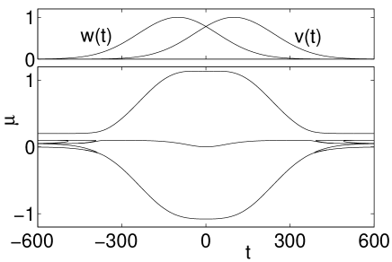
Figure 6: Eigenvalues of the nonlinear Hamiltonian (3) for a detuning $\Delta=0.1$ and a nonlinearity $g=0.2$ (lower panel) for time-dependent couplings $v(t)$ and $w(t)$ (upper panel).

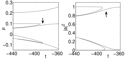
Figure 7: Left: Magnification of fig. 6. Right: Squared modulus of the first component ($|a_{\rm ad}|^{2}$) of the corresponding eigenstates. The avoided crossing that leads to a breakdown of adiabaticity is marked by an arrow.

However, the situation is more involved in the nonlinear case. To begin with we consider the case $g,\Delta>0$. As noted in the previous section, new nonlinear eigenstates emerge if the nonlinearity $|g|$ exceeds a critical value $g_{c}$ depending on the other sytem parameters. This can give rise to new crossing scenarios leading to a breakdown of adiabaticity. To illustrate this issue, the eigenvalues and eigenstates are calculated for a detuning $\Delta=0.1$ and $g=0.2$. The resulting adiabatic eigenvalues as well as the STIRAP pulse sequence of the couplings $v(t)$ and $w(t)$ are shown in fig. 6. At a first glance this picture looks quite similar to the linear case. The levels are shifted slightly due to the mean-field energy and a few additional nonlinear eigenvalues emerge for large $|t|$, because then the coupling elements $v$ and $w$ are small compared to the nonlinearity. However, a closer look at the adiabatic eigenvalues and eigenstates shown in fig. 7 reveals a fatal nonlinear avoided crossing scenario around $t\approx-380$, which will be referred to as the (avoided) ”horn crossing” in the following because of its shape. In the linear case the system’s dark state is rotated from $\psi_{\rm ds}(t=-\infty)=\psi_{1}$ to $\psi_{\rm ds}(t=+\infty))=\psi_{3}$, which leads to a coherent adiabatic population transfer. In the horn crossing however, this ”dark state” disappears when it merges with a nonlinear eigenstate (which will be referred to as horn state in the following), such that no adiabatic passage is possible any longer. To illustrate this breakdown of nonlinear STIRAP, we integrate the three-level NLSE numerically for the same parameters as in fig. 6. The resulting evolution of the populations $|a(t)|^{2}$ and $|c(t)|^{2}$ is shown in fig. 8 in comparison to the population $|a_{\rm ad}|^{2}$ of the instantaneous eigenstates. Due to the crossing, a state initially prepared in level $\psi_{1}$, $a(t=-\infty)=1$, cannot be transfered to level $\psi_{3}$ adiabatically any more. The dynamics follows the instantaneous eigenstate (the ”dark state”) adiabatically until this state disappears at the horn crossing. Fast oscillations of the populations $|a(t)|^{2}$ and $|c(t)|^{2}$ are observed afterwards. Finally the system settles down to a steady state again, but the population has not been transferred completely.

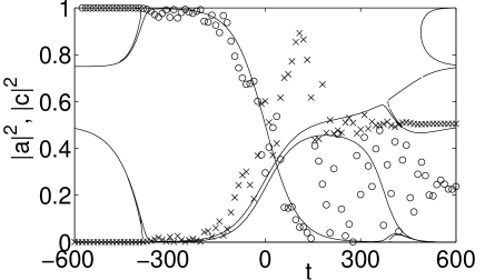
Figure 8: Time evolution of the population in the first ($|a(t)|^{2}$, open circles) and the third level ($|c(t)|^{2}$, crosses) in comparison with the population in the first level for the instantaneous eigenstates ($|a_{\rm ad}|^{2}$, solid lines) for $\Delta=0.1$ and $g=0.2$ and the couplings $v(t),w(t)$ shown in fig. 6 (upper panel).

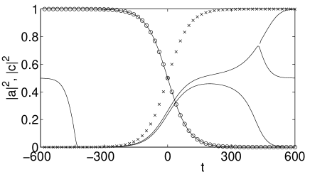
Figure 9: As fig. 8, however for $g=+0.05$.

For $g,\Delta>0$, it is found that the nonlinear eigenstate (the horn state) that merges with the dark state is a superposition of $\psi_{1}$ and $\psi_{2}$ alone in the limit $t\rightarrow-\infty$ and consequently $v,w\rightarrow 0$. Substitution of $c=0$ and $v=w=0$ into equation (4) immediately leads to

$$-\Delta+g|a|^{2}=\mu=g|b|^{2}.$$ (11)

Solving for $\Delta$ yields a condition for the existence of the horn state,

$$\Delta=g(|a|^{2}-|b|^{2})\leq g.$$ (12)

In this case a complete population transfer using the STIRAP scheme will be prevented by the horn crossing scenario discussed above. Nonlinear STIRAP is still possible if the nonlinearity is smaller than the detuning, $g<\Delta$. This is illustrated in fig. 9, where the evolution of the populations $|a(t)|^{2}$ and $|c(t)|^{2}$ is plotted in comparison to the population $|a_{\rm ad}|^{2}$ of the adiabatic eigenstates for $g=0.05$ and $\Delta=0.1$. One observes that the dynamics closely follows the adiabatic eigenstate and that the population is transferred from $\psi_{1}$ to $\psi_{3}$ completely. Note that the probability of Landau-Zener tunneling is also increased for $g<\Delta$ if the system parameters are varied at a finite velocity (cf. section III and ref. Wu00 ).

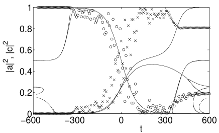
Figure 10: As fig. 8, however for $g=-0.2$.

An analogous situation is found for $g,\Delta<0$. However, a different crossing scenario arises if the signs of $\Delta$ and $g$ are opposite. Again the ”dark state” disappears when it merges with a nonlinear eigenstate (horn state). In this case it is found that the horn state is now a superposition of $\psi_{1}$ and $\psi_{3}$ alone in the limit $t\rightarrow-\infty$ as the dark state and that it exists for all values of $g$. Rigorously speaking, this leads to a breakdown of STIRAP even for very small nonlinearities. However, this crossing turns out to be not as fatal as the one discussed above; the transfer is still close to unity for weak nonlinearities (cf. fig. 11). An example of the dynamics is shown in fig. 10 for $\Delta=0.1$ and $g=-0.2$.

In conclusion we find the following conditions for the feasibility of a complete adiabatic population transfer using the STIRAP scheme:

$$g\Delta\geq 0\quad\mbox{and}\quad|g|<g_{c}=|\Delta|$$ (13)

The dependence of the transfer efficiency $|c(t\rightarrow+\infty)|^{2}$ on the nonlinearity is shown in fig. 11 for $\Delta=0.1$ and the same couplings $v(t)$ and $w(t)$ used in fig. 6 and 8. Note that exactly the same dependence is found if the signs of both $\Delta$ and $g$ are altered. The transfer efficiency is slightly reduced for all values $g<0$ and shows an oscillatory behavior. For $g>0$, one clearly observes an abrupt breakdown of the transfer efficiency above the critical nonlinearity, $g\geq g_{c}=|\Delta|$.

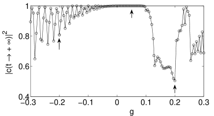
Figure 11: Numerically calculated transfer efficiency of nonlinear STIRAP in dependence of the nonlinearity $g$ for $\Delta=0.1$. The arrows indicate the values of $g$ for which the dynamics is shown in fig. 8, 9 and 10, respectively.

V Conclusion

In conclusion, the eigenstates and the dynamics generated by the nonlinear Hamiltonian (3) are analyzed for two important cases: the equal-slope Landau-Zener model and the STIRAP scheme. The emergence of new nonlinear eigenstates and novel crossing scenarios leads to a breakdown of adiabatic evolution if the nonlinearity $|g|$ exceeds a critical value. Consequently, STIRAP fails if the nonlinearity exceeds a critical value given by the detuning or if the nonlinear parameter and detuning have different signs. A novel feature of nonlinear Zener tunneling compared to the two-level system is the oscillatory behavior of the transition probability $P(\alpha)$. Open problems include a detailed analysis of the oscillations of $P(\alpha)$, the Landau-Zener scenario for non-equal slope and the effects of a parameter variation at finite velocity on the nonlinear STIRAP scheme.

- (1) L. Pitaevskii and S. Stringari, Bose-Einstein Condensation, Oxford University Press, Oxford, 2003
- (2) A. Smerzi, S. Fantoni, S. Giovanazzi, and S. R. Shenoy, Phys. Rev. Lett. 79 (1997) 4950
- (3) G. J. Milburn, J. Corney, E. M. Wright, and D. F. Walls, Phys. Rev. A 55 (1997) 4318
- (4) O. Zobay and B. M. Garraway, Phys. Rev. A 61 (2000) 033603
- (5) Biao Wu and Qian Niu, Phys. Rev. A 61 (2000) 023402
- (6) M. Holthaus, Phys. Rev. A 64 (2001) 011601
- (7) R. D’Agosta and C. Presilla, Phys. Rev. A 65 (2002) 043609
- (8) Biao Wu and Qian Niu, New J. Phys. 5 (2003) 104
- (9) E. M. Graefe, H. J. Korsch, K. Rapedius, and D. Witthaut, in preparation (2005)
- (10) A. Vardi, V. A. Yurovsky, and J. R. Anglin, Phys. Rev. A 64 (2001) 063611; A. Vardi and J. R. Anglin, Phys. Rev. Lett. 86 (2001) 568; J. R. Anglin and A.Vardi, Phys. Rev. A 64 (2001) 013605
- (11) R. K. Dodd, J. C. Eilbeck, J. D. Gibbon, and H. C. Morris, Solitons and nonlinear wave equations, Academic Press, London, 1982
- (12) A. Chefles and S. M. Barnett, J. Mod. Opt. 43 (1996) 709
- (13) B. Esser and H. Schanz, Z. Phys. B 96 (1995) 553
- (14) K. Winkler, G. Thalhammer, M. Theis, H. Ritsch, R. Grimm, and J. Hecker Denschlag, preprint: cond-mat/0505732 (2005)
- (15) J. Liu, B. Wu, and Q. Niu, Phys. Rev. Lett. 90 (2003) 170404
- (16) K. Bergmann, H. Theuer, and B.W. Shore, Rev. Mod. Phys. 70 (1998) 1003
- (17) K. Eckert, M. Lewenstein, R. Corbalan, G. Birkl, W. Ertmer, and J. Mompart, Phys. Rev. A 70 (2004) 023606
- (18) T. Poston and I. Stewart, Catastrope Theory and its Applications, Pitman, London, 1978
- (19) V. I. Arnold, Gewöhnliche Differentialgleichungen, § 5.4, Springer, New York, 1980
- (20) Q. Thommen, J. C. Garreau, and V. Zehnlé, Phys. Rev. Lett. 91 (2003) 210405
- (21) S. Brundobler and V. Elser, J. Phys. A 26 (1993) 1211
- (22) A. Messiah, Quantum Mechanics, Dover, Mineola, New York, 1999
- (23) C. Zener, Proc. Roy. Soc. Lond. A 145 (1934) 523
- (24) Y. N. Demkov, Sov. Phys.-Dokl. 11 (1966) 138
- (25) Y. N. Demkov and V. I. Osherov, Sov. Phys. JETP 26 (1968) 916
- (26) N. V. Vitanov, T. Halfmann, B.W. Shore, and K. Bergmann, Ann. Rev. Phys. Chem. 52 (2001) 763; F. Vewinger, M. Heinz, R. G. Fernandez, N. V. Vitanov, and K Bergmann, Phys. Rev. Lett. 91 (2003) 213001; M. Heinz, F. Vewinger, U. Schneider, and K. Bergmann, in preparation (2005)