Quantum Information Processing in Disordered and Complex Quantum Systems

Abstract

We investigate quantum information processing and manipulations in disordered systems of ultracold atoms and trapped ions. First, we demonstrate generation of entanglement and local realization of quantum gates in a quantum spin glass system. Entanglement in such systems attains significantly high values, after quenched averaging, and has a stable positive value for arbitrary times. Complex systems with long range interactions, such as ion chains or dipolar atomic gases, can be modeled by neural network Hamiltonians. In such systems, we find the characteristic time of persistence of quenched averaged entanglement, and also find the time of its revival.

Successful implementations of quantum information processing (QIP) in atomic, molecular, or solid state systems typically demand very rigorous control of such systems general . This concerns both few qubit systems such as the Cirac-Zoller computer cirac with ions or photons experiments , as well as atomic gases in optical lattices jaksch . Despite a lot of progress, the demanded control in such systems is nowadays very hard to achieve daley . Recently QIP in systems with a limited knowledge of the parameters has also been proposed ripoll .

At the first sight, what we propose here sounds like contradictio in adjecto: QIP in quenched disordered or complex, ergo hardly controllable, systems. However, as we have recently shown, one can create controlled disorder in atomic gases in optical lattices and study, in an unconventional way, Anderson and Bose glasses in a Bose gas damski , or spin glasses with short range interactions in Fermi-Bose, or Bose-Bose mixtures sanpera . Using linear chains of trapped ions porras , or dipolar atomic gases Baranov , it is possible to realize complex spin systems with long-range interactions that may serve as model for classical and quantum neural networks marisa .

Disordered systems offer at least two possible advantages for QIP. First, they have typically a large number of different metastable (free) energy minima, as it happens in spin glasses (SG) parisi . Such states might be used to store information distributed over the whole system, similarly to neural network (NN) models amit . The information is thus naturally stored in a redundant way, like in error correcting schemes shor . Second, in disordered systems with long range interactions, the stored information is robust: metastable states have quite large basins of attraction in the thermodynamical sense.

We address here the simplest fundamental questions concerning QIP in disordered or complex systems: (i) Can one generate entanglement in such systems that would survive quenched averaging over long times? (ii) Can one realize quantum gates with reasonable fidelity? Here we answer both questions affirmatively considering both short and long range disordered systems.

First, we consider a short range disorder Ising Hamiltonian, the so-called Edwards-Anderson (E-A) model of spin glasses which can be straightforwardly implemented using atomic Bose-Fermi, or Bose-Bose mixtures in optical latticesbofe ; sanpera . We address the generation and evolution of nearest neighbor (nn) entanglement in this model. In the short range Ising model without disorder, it is possible to create cluster and graph states (i.e. entanglement) starting from an appropriate initial product state briegel . Here we show that, while the disorder averaged density matrix of two neighboring spins remains always separable, the disorder averaged entanglement (quantified by logarithmic negativity VidalWerner ) converges with time to a finite value. The generation of entanglement briegel as well as its evolution for arbitrary times in an Ising model without disorder but with long-range interactions, has also been addressed in Ref. briegelnew . There it was suggested the possibility of applying similar ideas to disordered systems. We show also that the quantum single-qubit Hadamard gate, can be realized in such system with significant (disorder averaged) fidelity.

Secondly, we consider complex systems with long range ($1/r^{3}$, or $1/r^{2}$) interactions, that can be realized for instance, in linear ion traps, using either local magnetic fields, as proposed by Wunderlich and coworkerschristoph , or by appropriately designed laser excitations porras . The corresponding Hamiltonian can be mapped into an Ising Neural Network (NN) model with weighted patterns amit . Those patterns can be used as qubit systems, with the information distributed over the chain. One can also include external parallel, or transverse fields in the model. We show that in such system, it is possible to generate long range bipartite entanglement that undergoes a series of collapses and revivals Eberly , whose times are found analytically. Finally we study also bipartite and tripartite entanglement dynamics in an infinite range Ising model without disorder.

Let us start with the Edwards-Anderson spin glass model described by

$$H_{E-A}=-\frac{1}{4}\sum_{\left\langle ij\right\rangle}J_{ij}\sigma^{z}_{i}\sigma^{z}_{j}.$$ (1)

Here $\sigma^{z}_{k}$ denotes the Pauli operator at the $k$th site, and $J_{ij}$’s describe nn couplings for an arbitrary lattice. In the E-A model these couplings are given by independent Gaussian variables with mean $J$ and variance $\sigma^{2}$. Starting from a pure product state of the form $|\Psi\rangle=\prod_{i}|+\rangle_{i}$, where $\left|\pm\right\rangle=(\left|0\right\rangle\pm\left|1\right\rangle)/\sqrt{2}$ briegelnew , we evaluate the entanglement after a finite time, where the density matrix is given by $\rho(t,\{J_{ij}\})=\exp\{-iH_{E-A}t\}|\Psi\rangle\langle\Psi|\exp\{+iH_{E-A}t\}$. The reduced density matrix for a nn pair is obtained by tracing over all other sites. For instance, the reduced density matrix for a 2D square lattice is given by

$$\varrho_{12}(t,\{J_{ij}\})=\frac{1}{4}\operatorname{{\bf 1}}\otimes\operatorname{{\bf 1}}+\frac{1}{4}\Big{[}e^{iJ_{12}t/2}$$

$$\Big{\{}\cos(J_{24}t/2)\cos(J_{26}t/2)\cos(J_{28}t/2)|00\rangle\langle 01|$$

$$+ \cos(J_{13}t/2)\cos(J_{15}t/2)\cos(J_{17}t/2)|00\rangle\langle 10|\Big{\}}$$

$$+ e^{-iJ_{12}t/2}\Big{\{}\cos(J_{13}t/2\cos(J_{15}t/2)\cos(J_{17}t/2)|01\rangle\langle 11|$$

$$+ \cos(J_{24}t/2)\cos(J_{26}t/2)\cos(J_{28}t/2)|10\rangle\langle 11|\Big{\}}$$

$$+ \cos(J_{13}t/2)\cos(J_{15}t/2)\cos(J_{17}t/2)\cos(J_{24}t/2)$$

$$\times \cos(J_{26}t/2)\cos(J_{28}t/2)\Big{\{}|00\rangle\langle 11|+|01\rangle\langle 10|\Big{\}}+\mbox{h.c.}\Big{]},$$

where $\operatorname{{\bf 1}}$ is the identity operator and the indices $3\ldots 8$ enumerate the six neighbors of 1 and 2. A similar expression can be obtained for the 1D lattice. In both cases, the averaging of the reduced state over $J_{ij}$’s (equivalent to reducing the average $\varrho_{12}(t,\{J_{ij}\})$) is separable. Note, however, that as always in physics of disordered systems, if we are interested in typical values of physical quantities such as free energy, entanglement, etc., we are obliged to perform a ”quenched” average, i.e. first calculate the quantity of interest and then average parisi (see also ekhaneo1 ; ekhaneo2 ).

To study entanglement, we use the logarithmic negativity (LN) VidalWerner . The LN of a bipartite state $\rho_{AB}$ is defined as $E_{LN}(\rho_{AB})=\log_{2}\|\rho_{AB}^{T_{A}}\|_{1}$, where $\|.\|_{1}$ is the trace norm, and $\rho_{AB}^{T_{A}}$ denotes the partial transpose of $\rho_{AB}$ with respect to the $A$-part Peres_Horodecki . Note that $\rho_{ij}(t)$ acts on $\mathbb{C}^{2}\otimes\mathbb{C}^{2}$. Consequently, a positive value of the LN implies that the state is entangled and distillable Peres_Horodecki ; Horodecki_distillable , while $E_{LN}=0$ implies separability Peres_Horodecki .

The entanglement in the spin glass model turns out to be an even function of the couplings. The temporal behavior of $E_{LN}(t)$ in a 2D square lattice is shown in Fig. 1 for two different cases of disorder: with frustration and without it. For $J=0$, $\sigma^{2}=1$, the system has randomly ferro- ($J>0$) and antiferro-magnetic ($J<0$) interactions and is strongly frustrated; $E_{LN}(t)$ is rapidly damped to a constant, and does not show any oscillations. This behaviour differs from the non-frustrated case $J=5$, $\sigma^{2}=1$, when $E_{LN}(t)$ exhibits oscillations with frequencies $\sim 1/J$. For short range interactions, the next-nearest neighbor entanglement vanishes, even before the averaging, for both 1D and 2D. To understand why entanglement converges in time to the same finite value in both the frustated and non-frustated cases, notice that as long as the distributions $J_{ij}$’s are sufficiently well-behaved, $J_{ij}t/2$ corresponds to a uniform distribution over $[0,2\pi]$ for large enough $t$.

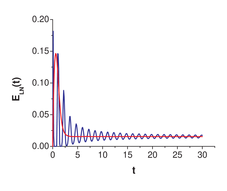
Figure 1: Temporal behavior of nn averaged entanglement in a 2D spin glass model, starting from $\Pi_{i}\left|+\right\rangle_{i}$. For a model with frustration ($J=0$), $E_{LN}(t)$ converges quickly to a constant value (red curve). For a non-frustrated case ($J=+5$), $E_{LN}(t)$ exhibits damped oscillations (blue curve), converging to the same value $\approx 0.0154$, as reached in the frustrated case. Standard deviation for $t\rightarrow\infty$ is $\approx 0.0704$. It is interesting to note that the dynamical behaviour of $E_{LN}$ depends on $J$, although at large times, they all converge to the same value.The same behavior is encountered in the 1D case, even though there is no frustration in that case.

We have calculated the nn entanglement for the following lattice configurations: 1D chain, 2D honey-comb lattice, 2D square, 3D cube, where any given pair of neighboring lattice sites has $d=2,4,6,10$ neighbors respectively. For time large enough, our numerics reveal that bipartite entanglement decays exponentially with the number of neighbors. Such behaviour can be reproduced analytically by considering the volume of the set of separable states (see e.g. KarolMaciek ), giving an upper bound on nn entanglement that depends exponentially on $d$. Some algebra shows that if the state $\rho_{ij}(t)$ is entangled, then $\sum_{i=1}^{d}\phi_{i}^{2}<(3-4R^{2})/2$, where the $\phi_{i}=J_{ij}t/2$’s are state parameters varying from 0 to $2\pi$, and $R$ is the radius of the separable ball in the $d$-dimensional space. The volume of this hypersphere is ${\cal V}_{d}={\cal S}_{d}\left(\frac{3-4R^{2}}{2}\right)^{\frac{d}{2}}/d$, where ${\cal S}_{d}=2\pi^{\frac{d}{2}}/\Gamma(d/2)$. Due to the periodicity involved implicitly in $\rho_{ij}(t)$, there are $2^{d}-1$ such hyperspheres. Considering all states in this volume to have unit entanglement, the average entanglement at long times is ${\cal E}_{d}={\cal V}_{d}(2^{d}-1)/(2\pi)^{d}$. As an example, for the case of the 2D lattice (for which $d=6$), at long times, the actual entanglement is $\approx 0.0154$, while ${\cal E}_{6}\approx 0.0221$. Although the bipartite entanglement vanishes with increasing number of neighbors, one can expect the multipartite entanglement to be non vanishing due to the fact that the volume of separable states is “super-doubly-exponentially small” with increasing number of parties dobol-chhoto .

We show now that spin glasses allows also to implement quantum gates. We focus on the Hadamard gate, which transforms the computational basis into a complementary basis: $\left|0\right\rangle\rightarrow\left|+\right\rangle$ and $\left|1\right\rangle\rightarrow\left|-\right\rangle$. To implement the Hadamard gate, assume that the computation is performed in a spin lattice, and the particles 1 and 2 are a part of it. We assume that at a certain time, particle 1 is in an arbitrary state $a|0\rangle+b|1\rangle$, where $|a|^{2}+|b|^{2}=1$, and we let system evolve according to the Hamiltonian $H_{E-A}$ for a suitable duration of time, before performing measurement on particle 1 (in a suitable basis). For $J=5,\sigma^{2}=1$, particle 2 attains the Hadamard rotated state $a|+\rangle+b|-\rangle$, with quenched averaged fidelity greater than $0.85$. One can increase such fidelity by increasing the number of spins, and employing assisted measurements. Note, that if we try to prepare the Hadamard rotated state using the classical information obtained only from the measurement of particle $1$, the fidelity is only $2/3$ classicalfidelity .

Let us now move to a long-range interactions spin Ising model, described by the Hamiltonian $H_{lr}=\frac{1}{N}\sum_{i,j}J_{ij}\sigma_{i}^{z}\sigma_{j}^{z}$, where $N$ is the total number of spins. Such models can be realized with trapped ions marisa , where $J_{ij}=\sum_{\mu}\xi^{i}_{\mu}\xi^{j}_{\mu}/\lambda_{\mu}^{2}$, with $\xi^{i}_{\mu}$ ($\lambda_{\mu}$) describing the phonon eigen-modes (eigen-frequencies). Here we consider two extreme cases. First, we take $\lambda_{1}=1,\xi_{1}^{i}=\mbox{constant}$ $\forall i$, $\lambda_{\mu}\rightarrow\infty$ for $\mu\geq 2$, so that the interactions are ordered, and the Hamiltonian is $H_{lro}=\frac{1}{N}S^{2}$, where $S=\sum_{i=1}^{N}\sigma^{z}_{i}$. Secondly, we consider the case when $\lambda_{\mu}=1$ for all $\mu$, when the Hamiltonian becomes $H_{NN}=\frac{1}{N}\sum_{i,j=1}^{N}\sum_{\mu=1}^{p}\xi^{(i)}_{\mu}\xi^{(j)}_{\mu}\sigma_{i}^{z}\sigma_{j}^{z}$. This is the Hopfield model of a neural network with Hebbian couplings amit . Here $p$ is the number of “patterns” of the neural network, and the patterns are described by random variables $\xi^{(i)}_{\mu}=\pm 1$, each with probability $\frac{1}{2}$. As in the case of short-range interactions, we take the initial state of the evolution as $|\Psi\rangle=\Pi_{i=1}^{N}|+\rangle_{i}$, and study the dynamics of entanglement for ordered and disordered Hamiltonians. We provide an efficient method to analytically compute the evolved state of any number of patterns and any number of spins.

Consider first the case of the Hamiltonian $H_{lro}$. We can write the evolution operator $\exp(-iS^{2}t/N)$ as $\int d\omega\exp((i/N)\omega^{2}+S\sqrt{t}(-2i/N)\omega)$, up to a constant factor. Applying now this unitary to the initial state $|\Psi\rangle$, we find any two-party state $\varrho_{12}^{lro}(t)=\operatorname{tr}_{k\neq 1,2}\rho^{lro}(t)$ of such system and compute the entanglement quantified by the LN. (This method can be also applied to find multipartite evolved states). In Fig 2, we plot the entanglement (as quantified by LN) of $\varrho^{lro}_{12}(t)$, with respect to time, as well as $N$. The figure shows revivals of bipartite entanglement, that occur on the time scale $\tau_{R}\sim N$, and persist on the time scale $\tau_{C}\sim\sqrt{N}$ (collapse time).

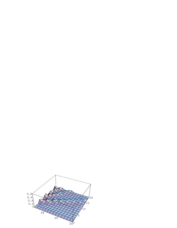
Figure 2: Generation of entanglement of bipartite states $\varrho^{lro}_{12}(t)$ with respect to time and number of spins. Collapses and revivals of the entanglement are clearly depicted.

As depicted in Fig. 2, there are large ranges of time, for which the bipartite state is separable. Interestingly, this range of separability can be reduced, considering entanglement of the tripartite evolved state $\rho_{123}^{lro}(t)$ in a bipartite cut. Although the interactions in $H_{lro}$ are long-range, they are ordered, so that $\rho_{12}^{lro}(t)$ and $\rho_{123}^{lro}(t)$ takes a relatively simple form. Amazingly, the same method applies for $H_{NN}$, where the interactions are both long-range and disordered. Despite its increased complexity, we can still use the technique for the evolution operator $\exp(-iH_{NN}t)$, that was used in the case of $H_{lro}$. Specifically, we replace in $\exp(-iH_{NN}t)$, the operator $\exp(-iS_{\mu}^{2}t/N)$ by $\int d\omega_{\mu}\exp((i/N)\omega_{\mu}^{2}+S_{\mu}\sqrt{t}(-2i/N)\omega_{\mu})$, for every $\mu$, where $S_{\mu}=\sum_{i=1}^{N}\xi^{(i)}_{\mu}\sigma_{i}^{z}$. Applying this operator to our initial state, we find that the $N$-particle state at time $t$ is

$$\varrho^{NN}(t)=\int(\Pi_{\mu}dr_{\mu}ds_{\mu}{{}^{\prime}})\mbox{e}^{i\sum_{\mu}r_{\mu}s_{\mu}/N}$$

$$\Pi_{i=1}^{N}\Big{[}\mbox{e}^{-2i\sqrt{t}\sum_{\mu}\xi_{\mu}^{(i)}s_{\mu}/N}(|0\rangle\langle 0|)_{i}$$

$$+\mbox{e}^{2i\sqrt{t}\sum_{\mu}\xi_{\mu}^{(i)}s_{\mu}/N}(|1\rangle\langle 1|)_{i}$$

$$+\Big{\{}\mbox{e}^{-2i\sqrt{t}\sum_{\mu}\xi_{\mu}^{(i)}r_{\mu}/N}(|0\rangle\langle 1|)_{i}+\mbox{h.c.}\Big{\}}\Big{]},$$ (3)

where $r_{\mu}=\omega_{\mu}+\omega_{\mu}{{}^{\prime}}$, $s_{\mu}=\omega_{\mu}-\omega_{\mu}{{}^{\prime}}$, with $\mu=1,\ldots,p$. After tracing out all except particles 1 and 2 we obtain:

$$\varrho {}^{NN}_{12}(t)=1/4\Big{\{}(|00\rangle\langle 00|+|01\rangle\langle 01|+|10\rangle\langle 10|+|11\rangle\langle 11|)$$ (4)

$$+ \Big{[}\mbox{e}^{-4it\sum_{\mu}\xi_{\mu}^{(1)}\xi_{\mu}^{(2)}/N}\Big{(}\Pi_{i\neq 1,2}\cos(4t\sum_{\mu}\xi_{\mu}^{(i)}\xi_{\mu}^{(2)}/N)|00\rangle\langle 01|$$

$$+ \Pi_{i\neq 1,2}\cos(4t\sum_{\mu}\xi_{\mu}^{(i)}\xi_{\mu}^{(1)}/N)|00\rangle\langle 10|\Big{)}\Big{]}$$

$$+ \Pi_{i\neq 1,2}\cos(4t\sum_{\mu}\xi_{\mu}^{(i)}(\xi_{\mu}^{(1)}+\xi_{\mu}^{(2)})/N)|00\rangle\langle 11|$$

$$+ \Pi_{i\neq 1,2}\cos(4t\sum_{\mu}\xi_{\mu}^{(i)}(\xi_{\mu}^{(1)}-\xi_{\mu}^{(2)})/N)|01\rangle\langle 10|$$

$$+ \Big{[}\mbox{e}^{4it\sum_{\mu}\xi_{\mu}^{(1)}\xi_{\mu}^{(2)}/N}\Big{(}\Pi_{i\neq 1,2}\cos(4t\sum_{\mu}\xi_{\mu}^{(i)}\xi_{\mu}^{(1)}|01\rangle\langle 11|$$

$$+ \Pi_{i\neq 1,2}\cos(4t\sum_{\mu}\xi_{\mu}^{(i)}\xi_{\mu}^{(2)}/N)|10\rangle\langle 11|\Big{)}\Big{]}+\mbox{h.c.}\Big{]}\Big{\}}.$$

For $N$ large, and $t/N$ small, the above expression can be simplified using the fact that $\Pi_{i\neq 1,2}\cos(4t\sum_{\mu}\xi_{\mu}^{(i)}\xi_{\mu}^{(2)}/N)=\exp\Big{[}\sum_{i\neq 1,2}\log_{e}|\cos(4t\sum_{\mu}\xi_{\mu}^{(i)}\xi_{\mu}^{(2)}/N)|\Big{]}=\exp[-(8t^{2}/N^{2})\sum_{i\neq 1,2}(\sum_{\mu}x^{i}_{\mu})^{2}]$, where for all $i$, $x^{i}_{\mu}=+1$ or $-1$ with probability $1/2$ each. Therefore, for large $N$ and small $t/N$, we have that $\Pi_{i\neq 1,2}\cos(4t\sum_{\mu}\xi_{\mu}^{(i)}\xi_{\mu}^{(2)}/N)$ self-averages to the value $\exp[-(8t^{2}p/N)]$, so that after time $t\sim\sqrt{N/p}$, all the off-diagonal elements of the state $\varrho^{NN}_{12}(t)$ become vanishingly small. Therefore, for the first time, nearest neighbor entanglement in the evolved state appears and persists for times of order $\tau_{C}\sim\sqrt{N/p}$. However, there are repeated revivals in entanglement, with the period being $\tau_{R}\simeq\pi N/2$ for odd $p$, and $\tau_{R}\simeq\pi N$ for even $p$. Note, that the period of revivals is independent of the number of patterns in the model (cf. ekhaneo2 ).

Summarizing, we have studied disordered and complex spin systems with short-range and long range interactions that can be realized with trapped atoms or ions. We have shown that in both cases it is possible to generate quenched averaged entanglement over long times. In the case of short range interactions, we considered Edwards-Anderson model in 1D and 2D square lattice. We have shown that in such disordered system, it is possible to implement also distinctly quantum single-qubit gates with high fidelity. We have also demonstrated that it is possible to generate entanglement in the spin system with long range interactions, corresponding to the Hopfield neural network model. We have shown that in such case, entanglement exhibits a sequence of collapses and revivals.

We thank I. Bloch, H.-P. Büchler, J. Eschner, M. Pons, L. Sanchez-Palencia, J. Wehr and P. Zoller for fruitful discussions. We acknowledge support from the Deutsche Forschungsgemeinschaft (SFB 407, SPP1078 and SPP1116, 436POL), the RTN Cold Quantum Gases, Ministerio de Ciencia y Tecnología BFM-2002-02588, the Alexander von Humboldt Foundation, the EC Program QUPRODIS, the ESF Program QUDEDIS, and EU IP SCALA.

References

- (1) Institució Catalana de Recerca i Estudis Avançats.
- (2) D. Bouwmeester, A. Ekert, and A. Zeilinger (Eds.), The Physics of quantum information (Springer, Berlin, 2000).
- (3) J.I. Cirac and P. Zoller, Phys. Rev. Lett. 74, 4091 (1995).
- (4) F. Schmidt-Kaler et al., Nature 422, 408 (2003); J. Chiaverini et al., Nature 432, 602 (2004); P. Walther et al., Nature 434, 169 (2005).
- (5) G.K. Brennen et al., Phys. Rev. Lett. 82, 1060 (1999); D. Jaksch et al., Phys. Rev. Lett. 85, 2208 (2000); O. Mandel et al., Nature 425, 937 (2003).
- (6) P. Rabl et al., Phys. Rev. Lett. 91, 110403 (2003).
- (7) J.J. Garcia-Ripoll and J.I. Cirac, Phys. Rev. Lett. 90, 127902 (2003).
- (8) B. Damski et al., Phys. Rev. Lett. 91, 080403 (2003).
- (9) A. Sanpera et al., Phys. Rev. Lett. 93, 040401 (2004).
- (10) D. Porras and J.I. Cirac, Phys. Rev. Lett. 92, 207901 (2004).
- (11) For a review see, M. Baranov et al., Phys. Scripta T102 74 (2002); for the first experiment see P.O. Schmidt et al., Phys. Rev. Lett. 91, 193201 (2003).
- (12) M.L. Pons et al. in preparation.
- (13) M. Mézard, G. Parisi, and M.A. Virasoro, Spin Glass and Beyond (World Scientific, Singapore, 1987).
- (14) D.J. Amit, Modeling Brain Function (Cambridge University Press, Cambridge, 1992).
- (15) P.W. Shor, Phys. Rev. A 52, R2493 (1995); A.M. Steane, Proc. R. Soc. London A, 452, 2551 (1996).
- (16) M. Lewenstein et al., Phys. Rev. Lett. 92, 050401 (2004).
- (17) H.J. Briegel and R. Raussendorf, Phys. Rev. Lett. 86, 910 (2001); R. Raussendorf and H.J. Briegel, ibid. 86, 5188 (2001); R. Raussendorf, D.E. Browne, and H.J. Briegel, Phys. Rev. A 68, 022312 (2003).
- (18) G. Vidal and R.F. Werner, Phys. Rev. A, 65, 032314 (2002).
- (19) W. Dür et al., Phys. Rev. Lett. 94, 097203 (2005).
- (20) F. Mintert and C. Wunderlich, Phys. Rev. Lett. 87, 257904 (2001).
- (21) J.H. Eberly, N.B. Narozhny, and J.J. Sanchez-Mondragon, Phys. Rev. Lett. 44, 1323 (1980).
- (22) J. Calsamiglia, L. Hartmann, W. Dür, H.J. Briegel, quant-ph/0502017.
- (23) L. Hartmann, J. Calsamiglia, W. Dür, H.J. Briegel, quant-ph/0506208.
- (24) A. Peres, Phys. Rev. Lett. 77, 1413 (1996); M. Horodecki, P. Horodecki, and R. Horodecki, Phys. Lett. A 223, 1 (1996).
- (25) M. Horodecki, P. Horodecki, and R. Horodecki Phys. Rev. Lett. 78, 574 (1997).
- (26) K. Życzkowski, P. Horodecki, A. Sanpera, and M. Lewenstein, Phys. Rev. A, 58, 883 (1998).
- (27) S. Szarek, quant-ph/0310061.
- (28) S. Popescu, Phys. Rev. Lett. 72, 797 (1994).