An Introduction to
Cartan’s KAK Decomposition
for QC Programmers

Abstract

This paper presents no new results; its goals are purely pedagogical. A special case of the Cartan Decomposition has found much utility in the field of quantum computing, especially in its sub-field of quantum compiling. This special case allows one to factor a general 2-qubit operation (i.e., an element of $U(4)$) into local operations applied before and after a three parameter, non-local operation. In this paper, we give a complete and rigorous proof of this special case of Cartan’s Decomposition. From the point of view of QC programmers who might not be familiar with the subtleties of Lie Group Theory, the proof given here has the virtues, that it is constructive in nature, and that it uses only Linear Algebra. The constructive proof presented in this paper is implemented in some Octave/Matlab m-files that are included with the paper. Thus, this paper serves as documentation for the attached m-files.

1 Introduction and Motivation

Cartan’s KAK Decomposition was discovered by the awesome mathematical genius, Elie Cartan (1869-1951). Henceforth, for succinctness, we will refer to his decomposition merely as KAK. The letters KAK come from the fact that in stating and proving KAK, one considers a group $\underline{G}=\exp(\underline{g})$ with a subgroup $\underline{K}=\exp(\underline{k})$ and a Cartan subalgebra $\underline{a}$, where $\underline{g}=\underline{k}\oplus\underline{k}^{\perp}$ and $\underline{a}\subset\underline{k}^{\perp}$. Then one shows that any $G\in\underline{G}$ can be expressed as $G=K_{1}AK_{2}$, where $K_{1},K_{2}\in\underline{K}$ and $A\in\exp(\underline{a})$. An authoritative discussion of KAK can be found in the book by Helgason[1].

KAK was first applied to quantum computing (QC) by Khaneja and Glaser in Refs.[2]. Since we are using “KAK” to refer to the general theorem, we will use “KAK1” to refer to the special case of KAK used by Khaneja and Glaser. Besides KAK1, the Cosine-Sine Decomposition (CSD)[3][4] is another decomposition that is very useful[5] in QC. After Refs.[2] and [5], QC workers came to the realization[6] that CSD also follows from KAK , even though CSD was discovered[4] quite independently from KAK.

This paper will only discuss KAK1. KAK1 is the assertion that: Given any $U\in SU(4)$, one can find $A_{1},A_{0},B_{1},B_{0}\in SU(2)$ and $\vec{k}\in{\mathbb{R}}^{3}$ so that

$$U=(A_{1}\otimes A_{0})e^{i\vec{k}\cdot\vec{\Sigma}}(B_{1}\otimes B_{0})\;,$$ (1)

where $\vec{\Sigma}$ is an operator that is independent of $U$ and will be defined later. Thus KAK1 parameterizes $SU(4)$, a 15-parameter Lie Group, so that 12 parameters characterize local operations, and only 3 parameters (the 3 components of $\vec{k}$) characterize non-local ones.

Ever since Refs.[2] appeared, many workers other than Khaneja and Glaser have used KAK1 in QC to great advantage (see, for example, Refs.[7], [8], [9]). Mainly, they have used KAK1 to compile 2-qubit operations. For instance, Vidal and Dawson used KAK1 to prove that any 2-qubit operation can be expressed with 3 or fewer CNOTs and some 1-qubit rotations.

This paper includes a complete, rigorous proof of KAK1 and related theorems. The proof of KAK1 presented here is based on the well known isomorphism $SO(4)=\frac{SU(2)\times SU(2)}{\{(1,1),(-1-1)\}}$ and on a theorem by Eckart and Young (EY)[10]. The EY theorem gives necessary and sufficient conditions for simultaneous SVD (singular value decomposition) of two matrices. The relevance of the EY theorem to KAK1 was pointed out in Ref.[11]. The proof of KAK1 given here is a constructive proof, and it uses only Linear Algebra. Contrast this to the proof of KAK given in Ref.[1], which, although much more general, is a non-constructive (“existence”) proof, and it uses advanced concepts in Lie Group Theory.

Octave is a programming environment and language that is gratis and open software. It copies most of Matlab’s function names and capabilities in Linear Algebra. A collection of Octave/Matlab m-files that implement the algorithms in this paper, can be found at ArXiv (under the “source” for this paper), and at my website (www.ar-tiste.com).

2 Notation and Other Preliminaries

In this section, we will define some notation that is used throughout this paper. For additional information about our notation, see Ref.[12].

We will use the word “ditto” to mean likewise and respectively. For example, “$x$ (ditto, $y$) is in $A$ (ditto, $B$)”, means $x$ is in $A$ and $y$ is in $B$.

As usual, ${\mathbb{R}},{\mathbb{C}}$ will stand for the real and complex numbers. For any complex matrix $A$, the symbols $A^{*},A^{T},A^{\dagger}$ will stand for the complex conjugate, transpose, and Hermitian conjugate, respectively, of $A$. (Hermitian conjugate a.k.a. conjugate transpose and adjoint)

The Pauli matrices are defined by:

$${\sigma_{X}}=\left(\begin{array}[]{cc}0&1\\ 1&0\end{array}\right)\;,\;\;{\sigma_{Y}}=\left(\begin{array}[]{cc}0&-i\\ i&0\end{array}\right)\;,\;\;{\sigma_{Z}}=\left(\begin{array}[]{cc}1&0\\ 0&-1\end{array}\right)\;.$$ (2)

They satisfy

$${\sigma_{X}}{\sigma_{Y}}=-{\sigma_{Y}}{\sigma_{X}}=i{\sigma_{Z}}\;,$$ (3)

and the two other equations obtained from this one by permuting the indices $(x,y,z)$ cyclically. We will also have occasion to use the operator $\vec{\sigma}$, defined by:

$$\vec{\sigma}=({\sigma_{X}},{\sigma_{Y}},{\sigma_{Z}})\;.$$ (4)

Let $\sigma_{X_{\mu}}$ for $\mu\in\{0,1,2,3\}$ be defined by $\sigma_{X_{0}}=\sigma_{1}=I_{2}$, where $I_{2}$ is the 2 dimensional identity matrix, $\sigma_{X_{1}}={\sigma_{X}}$, $\sigma_{X_{2}}={\sigma_{Y}}$, and $\sigma_{X_{3}}={\sigma_{Z}}$. Now define

$$\sigma_{X_{\mu}X_{\nu}}=\sigma_{X_{\mu}}\otimes\sigma_{X_{\nu}}\;$$ (5)

for $\mu,\nu\in\{0,1,2,3\}$. For example, ${\sigma_{XY}}={\sigma_{X}}\otimes{\sigma_{Y}}$ and ${\sigma_{1X}}=I_{2}\otimes{\sigma_{X}}$. The matrices $\sigma_{X_{\mu}X_{\nu}}$ satisfy

$${\sigma_{XX}}{\sigma_{YY}}={\sigma_{YY}}{\sigma_{XX}}=-{\sigma_{ZZ}}\;,$$ (6)

and the two other equations obtained from this one by permuting the indices $(x,y,z)$ cyclically. We will also have occasion to use the operator $\vec{\Sigma}$, defined by:

$$\vec{\Sigma}=({\sigma_{XX}},{\sigma_{YY}},{\sigma_{ZZ}})\;.$$ (7)

Define

$${\cal M}=\frac{1}{\sqrt{2}}\left(\begin{array}[]{cccc}1&0&0&i\\ 0&i&1&0\\ 0&i&-1&0\\ 1&0&0&-i\end{array}\right)\;.$$ (8)

It is easy to check that ${\cal M}$ is a unitary matrix. The columns of ${\cal M}$ are an orthonormal basis, often called the “magic basis” in the quantum computing literature. (That’s why we have chosen to call this matrix ${\cal M}$, because of the “m” in magic).

In this paper, we often need to find the outcome ${\cal M}^{\dagger}X{\cal M}$ (or ${\cal M}X{\cal M}^{\dagger}$) of a similarity transformation ( equivalent to a change of basis) of a matrix $X\in{\mathbb{C}}^{4\times 4}$ with respect to ${\cal M}$. Since $X$ can always be expressed as a linear combination of the $\sigma_{X_{\mu}X_{\nu}}$, it is useful to know the outcomes ${\cal M}^{\dagger}(\sigma_{X_{\mu}X_{\nu}}){\cal M}$ (or ${\cal M}(\sigma_{X_{\mu}X_{\nu}}){\cal M}^{\dagger}$) for $\mu,\nu\in\{0,1,2,3\}$. One finds the following two tables:

$${\cal M}^{\dagger}(A\otimes B){\cal M}=\;\;\;\;\begin{array}[]{|rr|rrrr|}\hline\cr&&&B&\rightarrow&\\ &&1&{\sigma_{X}}&{\sigma_{Y}}&{\sigma_{Z}}\\ \hline\cr&1&1&-{\sigma_{1Y}}&{\sigma_{YZ}}&-{\sigma_{YX}}\\ A&{\sigma_{X}}&-{\sigma_{ZY}}&{\sigma_{Z1}}&-{\sigma_{XX}}&-{\sigma_{XZ}}\\ \downarrow&{\sigma_{Y}}&-{\sigma_{Y1}}&{\sigma_{YY}}&-{\sigma_{1Z}}&{\sigma_{1X}}\\ &{\sigma_{Z}}&-{\sigma_{XY}}&{\sigma_{X1}}&{\sigma_{ZX}}&{\sigma_{ZZ}}\\ \hline\cr\end{array}\;,$$ (9)

$${\cal M}(A\otimes B){\cal M}^{\dagger}=\;\;\;\;\begin{array}[]{|rr|rrrr|}\hline\cr&&&B&\rightarrow&\\ &&1&{\sigma_{X}}&{\sigma_{Y}}&{\sigma_{Z}}\\ \hline\cr&1&1&{\sigma_{YZ}}&-{\sigma_{1X}}&-{\sigma_{YY}}\\ A&{\sigma_{X}}&{\sigma_{ZX}}&-{\sigma_{XY}}&-{\sigma_{Z1}}&-{\sigma_{XZ}}\\ \downarrow&{\sigma_{Y}}&-{\sigma_{Y1}}&-{\sigma_{1Z}}&{\sigma_{YX}}&{\sigma_{1Y}}\\ &{\sigma_{Z}}&{\sigma_{XX}}&{\sigma_{ZY}}&-{\sigma_{X1}}&{\sigma_{ZZ}}\\ \hline\cr\end{array}\;.$$ (10)

3 Proof of KAK1

In this section, we present a proof of KAK1 and related theorems. The proofs are constructive in nature and yield the algorithms used in our software for calculating KAK1. Thus, even those persons that are not too enamored with mathematical proofs may benefit from reading this section.

Theorem 1

Define a map $\phi$ by

$$\phi:SU(2)\rightarrow SO(3)\;,\;\;\phi(A)={\cal M}^{\dagger}(A\otimes A^{*}){\cal M}\;.$$ (11)

Then $\phi$ is a well defined, onto, 2-1, homomorphism. Well-defined: For all $A\in SU(2)$, ${\cal M}^{\dagger}(A\otimes A^{*}){\cal M}\in SO(3)$. Onto: For all $Q\in SO(3)$, there exist $A\in SU(2)$ such that $Q={\cal M}^{\dagger}(A\otimes A^{*}){\cal M}$. 2-1: $\phi$ maps exactly two elements ($A$ and $-A$) into one ($\phi(A)$). Homomorphism: $\phi$ preserves group operations.

Theorem 2

Define a map $\Phi$ by

$$\Phi:SU(2)\times SU(2)\rightarrow SO(4)\;,\;\;\Phi(A,B)={\cal M}^{\dagger}(A\otimes B^{*}){\cal M}\;.$$ (12)

Then $\Phi$ is a well defined, onto, 2-1, homomorphism. Well-defined: For all $A,B\in SU(2)$, ${\cal M}^{\dagger}(A\otimes B^{*}){\cal M}\in SO(4)$. Onto: For all $Q\in SO(4)$, there exist $A,B\in SU(2)$ such that $Q={\cal M}^{\dagger}(A\otimes B^{*}){\cal M}$. 2-1: $\phi$ maps exactly two elements ($(A,B)$ and $(-A,-B)$) into one ($\phi(A,B)$). Homomorphism: $\Phi$ preserves group operations.

Theorems 1 and 2 are proven in most modern treatises on quaternions, albeit using a different language, the language of quaternions. See Version 2 or higher of Ref.[12], for proofs of Theorems 1 and 2, given in the language favored here and within the quantum computing community.

Lemma 3

Suppose $X$ is a unitary matrix and define $X_{R}=\frac{X+X^{*}}{2}$, $X_{I}=\frac{X-X^{*}}{2i}$. Then $Q=\left(\begin{array}[]{cc}X_{R}&X_{I}\\ -X_{I}&X_{R}\end{array}\right)$ is an orthogonal matrix. Furthermore, $X_{R}$ and $X_{I}$ are real matrices satisfying $X_{R}X_{R}^{T}+X_{I}X_{I}^{T}=X_{R}^{T}X_{R}+X_{I}^{T}X_{I}=1$. Furthermore, $X_{I}X_{R}^{T}$ and $X_{I}^{T}X_{R}$ are both real, symmetric matrices.

proof:

$$1=XX^{\dagger}=(X_{R}+iX_{I})(X_{R}^{T}-iX_{I}^{T})\;,$$ (13)

so

$$X_{R}X_{R}^{T}+X_{I}X_{I}^{T}=1\;,$$ (14a)

and

$$X_{I}X_{R}^{T}-X_{R}X_{I}^{T}=0\;.$$ (14b)

From $1=X^{\dagger}X$ we also get

$$X_{R}^{T}X_{R}+X_{I}^{T}X_{I}=1\;,$$ (15a)

and

$$X_{I}^{T}X_{R}-X_{R}^{T}X_{I}=0\;.$$ (15b)

Note that Eqs.(14) and Eqs.(15) are identical except that in Eqs.(14), the second matrix of each product is transposed, whereas in Eqs.(15), the first is. $Q$ is clearly a real matrix, and Eqs.(14) imply that its columns are orthonormal. Hence $Q$ is orthogonal. Eq.(14b) (ditto, Eq.(15b)) implies that $X_{I}X_{R}^{T}$ (ditto, $X_{I}^{T}X_{R}$) is symmetric.
QED

The next theorem, due to Eckart and Young, gives necessary and sufficient conditions for finding a pair of unitary matrices $U,V$ that simultaneously accomplish the SVD (singular value decomposition) of two same-sized but otherwise arbitrary matrices $A$ and $B$. The proof reveals that the problem of finding simultaneous SVD’s can be reduced to the simpler problem of finding simultaneous diagonalizations of two commuting Hermitian matrices. The problem of simultaneously diagonalizing two commuting Hermitian operators (a.k.a. observables) is well known to physicists from their study of Quantum Mechanics.

Theorem 4

(Eckart-Young) Suppose $A,B$ are two complex (ditto, real) rectangular matrices of the same size. There exist two unitary (ditto, orthogonal) matrices $U,V$ such that $D_{1}=U^{\dagger}AV$ and $D_{2}=U^{\dagger}BV$ are both real diagonal matrices if and only if $AB^{\dagger}$ and $A^{\dagger}B$ are Hermitian (ditto, real symmetric) matrices.

proof:

($\Rightarrow$) $AB^{\dagger}=UD_{1}D_{2}U^{\dagger}$ and $A^{\dagger}B=VD_{1}D_{2}V^{\dagger}$ so they are Hermitian.

($\Leftarrow$)Let

$$A^{\prime}=U_{A}^{\dagger}AV_{A}=\left(\begin{array}[]{cc}D&0_{2}\\ 0_{3}&0_{4}\end{array}\right)\;$$ (16)

be a SVD of $A$. Thus, $U_{A},V_{A}$ are unitary matrices, $0_{2},0_{3},0_{4}$ are zero matrices, and $D$ is a square diagonal matrix whose diagonal elements are strictly positive. Let

$$B^{\prime}=U_{A}^{\dagger}BV_{A}=\left(\begin{array}[]{cc}G&K\\ L&H\end{array}\right)\;,$$ (17)

where $D$ and $G$ are square matrices of the same dimension, $rank(A)$. Note that

$$A^{\prime}B^{{}^{\prime}\dagger}=B^{\prime}A^{{}^{\prime}\dagger}\Rightarrow\left(\begin{array}[]{cc}DG^{\dagger}&DL^{\dagger}\\ 0&0\end{array}\right)=\left(\begin{array}[]{cc}GD&0\\ LD&0\end{array}\right)\;,$$ (18)

and

$$A^{{}^{\prime}\dagger}B^{\prime}=B^{{}^{\prime}\dagger}A^{\prime}\Rightarrow\left(\begin{array}[]{cc}DG&DK\\ 0&0\end{array}\right)=\left(\begin{array}[]{cc}G^{\dagger}D&0\\ K^{\dagger}D&0\end{array}\right)\;.$$ (19)

Therefore,

$$L=K=0\;,$$ (20)

and

$$DG^{\dagger}=GD\;,\;\;DG=G^{\dagger}D\;.$$ (21)

When written in index notation, Eqs.(21) become

$$d_{i}g^{*}_{ji}=g_{ij}d_{j}\;,\;\;d_{i}g_{ij}=g^{*}_{ji}d_{j}\;,$$ (22)

where the indices range over $\{1,2,\ldots,rank(A)\}$. Eqs.(22) imply

$$(d_{i}+d_{j})(g^{*}_{ji}-g_{ij})=0\;.$$ (23)

Since $d_{i}>0$, we conclude that $G$ is a Hermitian matrix. $D$ is Hermitian too, and, by virtue of Eq.(21), $D$ and $G$ commute. Thus, these two commuting observables can be diagonalized simultaneously. Let $P$ be a unitary matrix that accomplishes this diagonalization:

$$D=P^{\dagger}DP\;,\;\;D_{G}=P^{\dagger}GP\;.$$ (24)

Let

$$D_{H}=U_{H}^{\dagger}HV_{H}\;$$ (25)

be a SVD of $H$. $D_{H}$ is a diagonal matrix with non-negative diagonal entries and $U_{H},V_{H}$ are unitary matrices. Now let

$$U^{\dagger}=\left(\begin{array}[]{cc}P^{\dagger}&0\\ 0&U^{\dagger}_{H}\end{array}\right)U^{\dagger}_{A}\;,\;\;V=V_{A}\left(\begin{array}[]{cc}P&0\\ 0&V_{H}\end{array}\right)\;.$$ (26)

The matrices $U$ and $V$ defined by Eq.(26) can be taken to be the matrices $U$ and $V$ defined in the statement of the theorem.
QED

Corollary 5

If $X$ is a unitary matrix, then there exist orthogonal matrices $Q_{L}$ and $Q_{R}$ and a diagonal unitary matrix $e^{i\Theta}$ such that $X=Q_{L}e^{i\Theta}Q_{R}^{T}$.

proof: Let $X_{R}$ and $X_{I}$ be defined as in Lemma 3. According to Lemma 3, $X_{I}X_{R}^{T}$ and $X_{I}^{T}X_{R}$ are real symmetric matrices, so we can apply Theorem 4 with $A=X_{R}$ and $B=X_{I}$. Thus, there exist orthogonal matrices $Q_{R}$ and $Q_{L}$ such that

$$D_{R}=Q_{L}^{T}X_{R}Q_{R}\;,\;\;D_{I}=Q_{L}^{T}X_{I}Q_{R}\;,$$ (27)

where $D_{R},D_{I}$ are real diagonal matrices. Since $X$ is unitary, $D_{R}+iD_{I}$ is too. Thus, we can define a diagonal unitary matrix $e^{i\Theta}$ by

$$e^{i\Theta}=D_{R}+iD_{I}\;.$$ (28)

Combining Eqs.(27) and (28) finally yields

$$e^{i\Theta}=Q_{L}^{T}XQ_{R}\;.$$ (29)

QED

Let $t=(\theta_{1},\theta_{2},\theta_{3},\theta_{4})\in{\mathbb{R}}^{4}$ and $\Theta=diag(t)$ so that

$$e^{i\Theta}=diag(e^{i\theta_{1}},e^{i\theta_{2}},e^{i\theta_{3}},e^{i\theta_{4}})\;.$$ (30)

Let $(k_{0},\vec{k})\in{\mathbb{R}}^{4}$. According to Eq.(9),

$${\cal M}^{\dagger}e^{i(k_{0}+\vec{k}\cdot\vec{\Sigma})}{\cal M}=e^{i(k_{0}+k_{1}{\sigma_{Z1}}-k_{2}{\sigma_{1Z}}+k_{3}{\sigma_{ZZ}})}\;.$$ (31)

If we set

$$e^{i\Theta}={\cal M}^{\dagger}e^{i(k_{0}+\vec{k}\cdot\vec{\Sigma})}{\cal M}\;,$$ (32)

then each point $(\theta_{1},\theta_{2},\theta_{3},\theta_{4})\in{\mathbb{R}}^{4}$ is mapped in a 1-1 onto fashion into each point $(k_{0},\vec{k})\in{\mathbb{R}}^{4}$. Using the explicit forms of ${\sigma_{Z1}},{\sigma_{1Z}},{\sigma_{ZZ}}$, one finds that

$$\left(\begin{array}[]{c}\theta_{0}\\ \theta_{1}\\ \theta_{2}\\ \theta_{3}\end{array}\right)=\Gamma\left(\begin{array}[]{c}k_{0}\\ k_{1}\\ k_{2}\\ k_{3}\end{array}\right)\;,\;\;{\rm where}\;\;\Gamma=\left(\begin{array}[]{cccc}+1&+1&-1&+1\\ +1&+1&+1&-1\\ +1&-1&-1&-1\\ +1&-1&+1&+1\end{array}\right)\;.$$ (33)

It is easy to check that

$$\Gamma^{-1}=\frac{\Gamma^{T}}{4}\;.$$ (34)

Corollary 6

(KAK1) If $X\in U(4)$, then $X=(A_{1}\otimes A_{0})e^{i(k_{0}+\vec{k}\cdot\vec{\Sigma})}(B_{1}\otimes B_{0})$, where $A_{1},A_{0},B_{1},B_{0}\in SU(2)$ and $(k_{0},\vec{k})\in{\mathbb{R}}^{4}$.

proof: Let

$$X^{\prime}={\cal M}^{\dagger}X{\cal M}\;.$$ (35)

$X^{\prime}$ is a unitary matrix, so, according to Collorary 5, we can find orthogonal matrices $Q_{L},Q_{R}$ and a diagonal unitary matrix $e^{i\Theta}$ such that

$$X^{\prime}=Q_{L}e^{i\Theta}Q_{R}^{T}\;.$$ (36)

According to Theorem 2, we can find $A_{1},A_{0},B_{1},B_{0}\in SU(2)$ such that

$${\cal M}Q_{L}{\cal M}^{\dagger}=A_{1}\otimes A_{0}\;,$$ (37)

and

$${\cal M}Q_{R}{\cal M}^{\dagger}=B_{1}\otimes B_{0}\;.$$ (38)

As in Eq.(32), set

$${\cal M}e^{i\Theta}{\cal M}^{\dagger}=e^{i(k_{0}+\vec{k}\cdot\vec{\Sigma})}\;.$$ (39)

It follows that

$$X=(A_{1}\otimes A_{0})e^{i(k_{0}+\vec{k}\cdot\vec{\Sigma})}(B_{1}\otimes B_{0})\;.$$ (40)

QED

4 Canonical Class Vector

In this section we discuss how KAK1 partitions $SU(4)$ into disjoint classes characterized by a 3d real vector $\vec{k}$.

We will say that $U,V\in SU(4)$ are equivalent up to local operations and write $U\sim V$ if $U=(R_{1}\otimes R_{0})V(S_{1}\otimes S_{0})$ where $R_{1},R_{0},S_{1},S_{0}\in U(2)$. It is easy to prove that $\sim$ is an equivalence relation. Hence, it partitions $SU(4)$ into disjoint subsets (i.e., equivalence classes). If $X\in SU(4)$ and $\vec{k}\in{\mathbb{R}}^{3}$ are related as in Collorary 6, then $X\sim e^{i\vec{k}\cdot\vec{\Sigma}}$. Henceforth, we will call this $\vec{k}$ a class vector of $X$. We will say that $\vec{k^{\prime}}$ and $\vec{k}$ are equivalent class vectors and write $\vec{k^{\prime}}\sim\vec{k}$ if $e^{i\vec{k^{\prime}}\cdot\vec{\Sigma}}\sim e^{i\vec{k}\cdot\vec{\Sigma}}$.

Note that the following 3 operations map a class vector into another class vector of the same class; i.e., the operations are class-preserving.

1. (Shift) Suppose we shift $\vec{k}$ by plus or minus $\frac{\pi}{2}$ along any one of its 3 components. For example, a positive, $\frac{\pi}{2}$, X-shift would map

   $$(k_{x},k_{y},k_{z})\mapsto(k_{x}+\frac{\pi}{2},k_{y},k_{z})\;.$$ (41)

   This operation preserves $\vec{k}$’s class because

   $$e^{i[(k_{x}+\frac{\pi}{2}){\sigma_{XX}}+k_{y}{\sigma_{YY}}+k_{z}{\sigma_{ZZ}}]}=e^{i\frac{\pi}{2}{\sigma_{XX}}}e^{i\vec{k}\cdot\vec{\Sigma}}\\ =i{\sigma_{XX}}e^{i\vec{k}\cdot\vec{\Sigma}}\;.$$ (42)

2. (Reverse) Suppose we reverse the sign of any two components of $\vec{k}$. For example, an XY-reversal would map

   $$(k_{x},k_{y},k_{z})\mapsto(-k_{x},-k_{y},k_{z})\;.$$ (43)

   This operation preserves $\vec{k}$’s class because

   $${\sigma_{Z1}}e^{i\vec{k}\cdot\vec{\Sigma}}{\sigma_{Z1}}=e^{i(-k_{x},-k_{y},k_{z})\cdot\vec{\Sigma}}\;.$$ (44)

3. (Swap) Suppose we swap any two components of $\vec{k}$. For example, an XY-swap would map

   $$(k_{x},k_{y},k_{z})\mapsto(k_{y},k_{x},k_{z})\;.$$ (45)

   This operation preserves $\vec{k}$’s class because

   $$e^{-i\frac{\pi}{4}({\sigma_{Z1}}+{\sigma_{1Z}})}e^{i\vec{k}\cdot\vec{\Sigma}}e^{i\frac{\pi}{4}({\sigma_{Z1}}+{\sigma_{1Z}})}=e^{i(k_{y},k_{x},k_{z})\cdot\vec{\Sigma}}\;.$$ (46)

Define ${\cal K}$ as the set of points $\vec{k}\in{\mathbb{R}}^{3}$ such that

1. $\frac{\pi}{2}>k_{x}\geq k_{y}\geq k_{z}\geq 0$

2. $k_{x}+k_{y}\leq\frac{\pi}{2}$

3. If $k_{z}=0$, then $k_{x}\leq\frac{\pi}{4}$.

${\cal K}$ is contained within the tetrahedral region $OA_{1}A_{2}A_{3}$ of Fig.1.

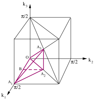
Figure 1: The set ${\cal K}$ of canonical class vectors equals the set of points in the tetrahedral region $OA_{1}A_{2}A_{3}$ (including all the interior and the surface points except that only the half $OBA_{2}$ of the base $OA_{1}A_{2}$ is included).

The 3 class-preserving operations given above generate a group $\underline{W}$. Given any class vector $\vec{k}\in{\mathbb{R}}^{3}$, it is always possible to find an operation $G\in\underline{W}$ such that $G(\vec{k})\in{\cal K}$. Indeed, here is an algorithm, (implemented in the accompanying Octave software) that finds $G(\vec{k})\in{\cal K}$ for any $\vec{k}\in{\mathbb{R}}^{3}$:

1. Make $k_{x}\in[0\frac{\pi}{2})$ by shifting $k_{x}$ repeatedly by $\frac{\pi}{2}$. In the same way, shift $k_{y}$ and $k_{z}$ into $[0\frac{\pi}{2})$.

2. Make $k_{x}\geq k_{y}\geq k_{z}$ by swapping the components of $\vec{k}$.

3. Perform this step iff at this point $k_{x}+k_{y}>\frac{\pi}{2}$. Transform $\vec{k}$ into $(\frac{\pi}{2}-k_{y},\frac{\pi}{2}-k_{x},k_{z})$ (This can be achieved by applying an XY-swap, XY-reverse, X-shift and Y-shift, in that order). At this point, $k_{x}\geq k_{y}$, but $k_{z}$ may be larger than $k_{y}$ or $k_{x}$, so finish this step by swapping coordinates until $k_{x}\geq k_{y}\geq k_{z}$ again.

4. Perform this step iff at this point $k_{z}=0$ and $k_{x}>\frac{\pi}{4}$. Transform $\vec{k}=(k_{x},k_{y},0)$ into $(\frac{\pi}{2}-k_{x},k_{y},0)$ (This can be achieved by applying an XZ-reverse and an X-shift, in that order).

We can find a subset $S$ of ${\mathbb{R}}^{3}$ such that every equivalence class of $SU(4)$ is represented by one and only one point $\vec{k}$ of $S$. In fact, ${\cal K}$ defined above is one such $S$. We will refer to the elements of ${\cal K}$ as canonical class vectors.

We end this section by finding the canonical class vectors of some simple 2-qubit operations.

1. (CNOT): $CNOT(1\rightarrow 0)$ is defined by

   $$CNOT(1\rightarrow 0)={\sigma_{X}}(0)^{n(1)}=\left(\begin{array}[]{cc}1&0\\ 0&{\sigma_{X}}\end{array}\right)\;.$$ (47)

   Since $n=\frac{1}{2}(1-{\sigma_{Z}})$, $n_{X}=\frac{1}{2}(1-{\sigma_{X}})$, and ${\sigma_{X}}=(-1)^{n_{X}}=e^{i\pi n_{X}}$,

   $${\sigma_{X}}(0)^{n(1)} = (-1)^{n_{X}(0)n(1)}$$ (48a)

   $$= e^{i\frac{\pi}{4}(1-{\sigma_{1X}})(1-{\sigma_{Z1}})}$$ (48b)

   $$= e^{i\frac{\pi}{4}(1-{\sigma_{Z1}}-{\sigma_{1X}})}e^{i\frac{\pi}{4}{\sigma_{ZX}}}$$ (48c)

   $$= e^{i\frac{\pi}{4}(1-{\sigma_{Z1}}-{\sigma_{1X}})}e^{i\frac{\pi}{4}{\sigma_{Y1}}}e^{i\frac{\pi}{4}{\sigma_{XX}}}e^{-i\frac{\pi}{4}{\sigma_{Y1}}}$$ (48d)

   $$\sim e^{i\frac{\pi}{4}{\sigma_{XX}}}\;.$$ (48e)

   Therefore, the canonical class vector of CNOT is $(\frac{\pi}{4},0,0)$, which corresponds to the point $B$ in Fig.1.

2. ($\sqrt{CNOT}$) From the math just performed for CNOT, it is clear that

   $$\sqrt{{\sigma_{X}}(0)^{n(1)}}=e^{i\frac{\pi}{8}(1-{\sigma_{1X}})(1-{\sigma_{Z1}})}\sim e^{i\frac{\pi}{8}{\sigma_{XX}}}\;.$$ (49)

   Therefore, the canonical class vector of $\sqrt{CNOT}$ is $(\frac{\pi}{8},0,0)$, which corresponds to the midpoint of the segment $OB$ in Fig.1.

3. (Exchanger, a.k.a. Swapper) As usual, the Exchanger is defined by

   $$E=\left(\begin{array}[]{cccc}1&0&0&0\\ 0&0&1&0\\ 0&1&0&0\\ 0&0&0&1\end{array}\right)\;.$$ (50)

   (Note that $\det(E)=-1$). Using Eqs.(6), it is easy to show that

   $$E=e^{-i\frac{\pi}{4}}e^{i\frac{\pi}{4}({\sigma_{XX}}+{\sigma_{YY}}+{\sigma_{ZZ}})}\;.$$ (51)

   Therefore, the canonical class vector of $e^{i\frac{\pi}{4}}E$ is $(\frac{\pi}{4},\frac{\pi}{4},\frac{\pi}{4})$, which corresponds to the apex $A_{3}$ of the tetrahedron in Fig.1.

5 Software

A collection of Octave/Matlab m-files that implement the algorithms in this paper, can be found at ArXiv (under the “source” for this paper), and at my website (www.ar-tiste.com). These m-files have only been tested on Octave, but they should run on Matlab with few or no modifications. A file called “m-fun-index.html” that accompanies the m-files lists each function and its purpose.

References

[1]
S. Helgason, Differential Geometry,
Lie Groups, and Symmetric Spaces (Am. Math. Soc.,
2001 edition, corrected reprint of 1978 original edition)
[2]
Navin Khaneja, Steffen Glaser,
“Cartan Decomposition of ,
Constructive Controllability
of Spin systems and
Universal Quantum Computing”,
quant-ph/0010100 .
Also
“Cartan decomposition of
and control of spin systems”,
Chemical Physics, 267
(2001), Pages 11-23.
[3]
G.H. Golub and C.F. Van Loan,
Matrix Computations, Third Edition
(John Hopkins Univ. Press, 1996).
[4]
C. C. Paige and M. Wei,
“History and Generality of
the CS Decomposition,”
Linear Algebra and Appl.
208/209(1994)303-326.