Harmonic entanglement with second-order non-linearity

Abstract

We investigate the second-order non-linear interaction as a means to generate entanglement between fields of differing wavelengths. And show that perfect entanglement can, in principle, be produced between the fundamental and second harmonic fields in these processes. Neither pure second harmonic generation, nor parametric oscillation optimally produce entanglement, such optimal entanglement is rather produced by an intermediate process. An experimental demonstration of these predictions should be imminently feasible.

Second-order nonlinear processes have found many applications in electronics, mechanics, optics, as well as numerous other fields. More recently, in the field of quantum optics it has been discovered that they offer an ideal mechanism for the generation of entangled states of light. As a result many fundamental theories of quantum mechanics have been tested at an unprecedented level AspectOu . It is surprising then to find that, to date, a comprehensive treatment of entanglement generated through second-order non-linear processes has not been presented. Here, we perform a broad analysis of entanglement in degenerate processes of this kind. We demonstrate that, in principle, perfect entanglement can be achieved between the fundamental and second harmonic fields involved in the process. This entanglement between harmonically related fields is referred to as harmonic entanglement. It is well known that quantum correlations and harmonic entanglement can be achieved via second harmonic generation (SHG) WisemanOlsen , and furthermore that highly squeezed states of light can be obtained in the complimentary process, optical parametric oscillation (OPO) Wu86 ; Lam . However, we find that optimal harmonic entanglement is not generated by either of these processes, but rather by an intermediate process, pump depleted optical parametric amplification (OPA). In contrast, previous investigations of the quantum optical properties of OPA have almost exclusively been limited to the small region of parameter space where pump depletion is insignificant.

The study of entangled states began as a means to test the counter intuitive predictions of the theory of quantum mechanics. In recent years, however, focus has shifted as a result of the realization that non-classical states of light can enhance many measurement, computation, and communication tasks Bennett ; Ralph . That quantum mechanics, in principle, allows such enhancement is significant in and of itself, and has motivated a great deal of theoretical work. However, emphasis has also been placed on experimental demonstrations, which as yet have been primitive by comparison. New tools are required for significant experimental progress to be made. Both SHG and OPO have found many applications in quantum optics experiments Lance ; Li ; Bowen03b , becoming standard tools in the field. The pump depleted OPA studied here has the potential to become equally significant. The generation of strong entanglement between optical fields at vastly different frequencies would immediately facilitate many interspecies quantum information protocols, for example the frequency of states of light could be drastically altered using interspecies quantum teleportation protocols. Such a protocol would enhance the integrability of disparate nodes in a quantum information network. Applications could be envisaged in any situation where a non-classical link is required between two experiments at differing optical frequencies. Such a situation might arise for example in experiments involving two different atomic species, or if a connection is required to an atomic frequency standard.

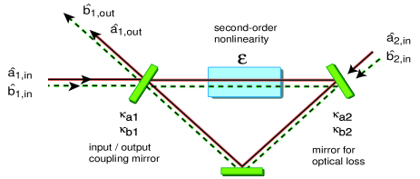
Figure 1: Schematic for the generation of optical harmonic entanglement.

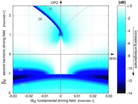
Figure 2: A plot of the EPR entanglement strength as a function of the fundamental, $\alpha$, and second harmonic, $\beta$, driving field amplitudes. Bi-stable OPA (i) above and (ii) below threshold. Parametric de-amplification regime (iii) above and (iv) below threshold.

Analysis: The system under analysis in this paper consists of a second order nonlinear medium enclosed within an optical resonator as shown in Fig. 1. The resonator is coupled to the environment through two partially reflective mirrors. One mirror represents an input/output coupler, while the other represents uncontrollable coupling loss. The non-linear medium induces an interaction between the two intra-cavity fields, giving Drummond

$$\begin{array}[]{ccl}\dot{\hat{a}}&=&-\kappa_{a}\hat{a}+\epsilon\hat{a}^{\dagger}\hat{b}+\hat{A}_{{\rm in}}\\ \dot{\hat{b}}&=&-\kappa_{b}\hat{b}-\frac{1}{2}\epsilon\hat{a}^{2}+\hat{B}_{{\rm in}},\end{array}$$ (1)

where $\hat{a}$ and $\hat{b}$ are Heisenberg picture annihilation operators describing the intra-cavity fundamental and second harmonic fields respectively; $\kappa_{a}$ and $\kappa_{b}$ are the associated total resonator decay rates; $\epsilon$ is the nonlinear coupling strength between the fields; and $\hat{A}_{\rm in}$ and $\hat{B}_{\rm in}$ represent the accumulated input fields to the system. Throughout this paper the partially reflective mirrors modeling input/output coupling and loss are distinguished with the subscripts ‘1’ and ‘2’, respectively; while the input and output fields are denoted by the subscripts ‘in’ and ‘out’. Using this terminology $\kappa_{a}=\kappa_{a1}+\kappa_{a2}$, $\kappa_{b}=\kappa_{b1}+\kappa_{b2}$, $\hat{A}_{{\rm in}}=\sqrt{2\kappa_{a1}}\hat{A}_{1,{\rm in}}+\sqrt{2\kappa_{a2}}\hat{A}_{2,{\rm in}}$, and $\hat{B}_{{\rm in}}=\sqrt{2\kappa_{b1}}\hat{B}_{1,{\rm in}}+\sqrt{2\kappa_{b2}}\hat{B}_{2,{\rm in}}$. The solution to Eqs. (1) is obtained through the technique of linearization, where operators are expanded in terms of their coherent amplitude and quantum noise operator, so that a mode $\hat{a}_{i}=\alpha+\delta\hat{a}_{i}$ with $\langle\delta\hat{a}_{i}\rangle=0$, and second order terms in the quantum noise operators are neglected. First, the steady state coherent amplitudes of the fundamental and second harmonic intra-cavity fields are obtained. After a stability analysis has been made on the solutions, the system shows a range of interesting behavior such as mono-stability, bi-stability, out-of-phase mono-stability, and self-pulsation Drummond . For clarity, we normalize the driving fields to their respective critical transition values, i.e. the critical amplitude, $\alpha_{1,{\rm in,c}}$, for self-pulsation in SHG, and the threshold amplitude $\beta_{1,{\rm in,c}}$ for OPO, such that

$$\alpha_{1,{\rm in,c}} = \frac{(2\kappa_{a}+\kappa_{b})[2\kappa_{b}(\kappa_{a}+\kappa_{b})]^{1/2}}{\epsilon\sqrt{2\kappa_{a1}}}$$ (2)

$$\beta_{1,{\rm in,c}} = \frac{\kappa_{a}\kappa_{b}}{\epsilon\sqrt{2\kappa_{b1}}}.$$ (3)

The normalized driving fields are then denoted $\alpha_{d}=\alpha_{1,{\rm in}}/\alpha_{1,{\rm in,c}}$ and $\beta_{d}=\beta_{1,{\rm in}}/\beta_{1,{\rm in,c}}$. The quantum fluctuations of the intra-cavity fields can be obtained from the fluctuating part of Eqs. (1)

$$\begin{array}[]{ccl}\delta\dot{\hat{a}}&=&-\kappa_{a}\delta\hat{a}+\epsilon(\alpha^{*}\delta\hat{b}+\beta\delta\hat{a}^{\dagger})+\hat{A}_{\rm in}\\ \delta\dot{\hat{b}}&=&-\kappa_{b}\delta\hat{b}-\epsilon\alpha\delta\hat{a}+\hat{B}_{\rm in}\end{array}$$ (4)

These equations can be easily solved by taking the Fourier transform into the frequency domain. We want to investigate harmonic entanglement between the amplitude $\hat{X}^{+}$ and phase $\hat{X}^{-}$ quadratures of the two output fields. These quadratures are related to the annihilation operators via $\hat{X}^{+}=\hat{a}+\hat{a}^{\dagger}$ and $\hat{X}^{-}=i(\hat{a}^{\dagger}-\hat{a})$. Writing the solution to Eqs. (4) in terms of field quadratures, we find

$$\left[\begin{array}[]{c}\delta X^{+}_{A,{\rm in}}\\ \delta X^{-}_{A,{\rm in}}\\ \delta X^{+}_{B,{\rm in}}\\ \delta X^{-}_{B,{\rm in}}\end{array}\right]=\left[\begin{array}[]{cccc}A&B&C&D\\ B&A^{\prime}&-D&C\\ -C&D&E&0\\ -D&-C&0&E\end{array}\right]\left[\begin{array}[]{c}\delta X^{+}_{a}\\ \delta X^{-}_{a}\\ \delta X^{+}_{b}\\ \delta X^{-}_{b}\end{array}\right]$$ (5)

where $\{\hat{X}^{\pm}_{a},\hat{X}^{\pm}_{b}\}$ and $\{\hat{X}^{\pm}_{A,{\rm in}},\hat{X}^{\pm}_{B,{\rm in}}\}$ are the intra-cavity and accumulated input field quadratures, respectively; and

$$A = \kappa_{a}-i\omega-\epsilon|\beta|\cos\theta_{\beta}$$ (6)

$$A^{\prime} = \kappa_{a}-i\omega+\epsilon|\beta|\cos\theta_{\beta}$$ (7)

$$B = -\epsilon|\beta|\sin\theta_{\beta}$$ (8)

$$C = -\epsilon|\alpha|\cos\theta_{\alpha}$$ (9)

$$D = -\epsilon|\alpha|\sin\theta_{\alpha}$$ (10)

$$E = \kappa_{b}-i\omega,$$ (11)

with $\theta_{\alpha}=\textrm{Arg}(\alpha),\theta_{\beta}=\textrm{Arg}(\beta)$, and $\omega$ is the side-band detection frequency. The fields output from the resonator can then be directly obtained using the input-output formalism, $\hat{X}^{\pm}_{{\rm A1,out}}\!=\!\sqrt{2\kappa_{a1}}\hat{X}^{\pm}_{a}\!-\!\hat{X}^{\pm}_{{{\rm A1,in}}}$, $\hat{X}^{\pm}_{{\rm B1,out}}\!=\!\sqrt{2\kappa_{b1}}\hat{X}^{\pm}_{b}\!-\!\hat{X}^{\pm}_{{{\rm B1,in}}}$ Collett . We can now proceed to investigate the presence of entanglement between the output fundamental and second harmonic fields. A bi-partite Gaussian entangled state is completely described by its correlation matrix Duan00 which has the following elements

$$C^{kl}_{mn}=\frac{1}{2}\langle\hat{X}^{k}_{m}\hat{X}^{l}_{n}+\hat{X}^{l}_{n}\hat{X}^{k}_{m}\rangle-\langle\hat{X}^{k}_{m}\rangle\langle\hat{X}^{l}_{n}\rangle$$ (12)

where $\{k,l\}\in\{+,-\}$ and $\{m,n\}\in\{\rm{A_{1,out}},\rm{B_{1,out}}\}$. The standard characterization of continuous variable entanglement is to measure the quantum correlations between two fields via the EPR criterion Reid88 and to apply the inseparability criterion Duan00 . Before the inseparability criterion can be applied however, the correlation matrix is required to be in standard form II, which can be achieved by application of the appropriate local-linear-unitary-Bogoliubov-operations (local rotation and squeezing operations) Duan00 . The product form of the degree of inseparability Bowen034 is given by

$$\mathcal{I}=\frac{\sqrt{C_{I}^{+}C_{I}^{-}}}{k^{2}+1/k^{2}},$$ (13)

where

$$C^{\pm}_{I}\!\!\! = \!\!\!\sqrt{\frac{C^{\pm\pm}_{bb}\!\!-\!\!1}{C^{\pm\pm}_{aa}\!\!-\!\!1}}C^{\pm\pm}_{aa}\!+\!\sqrt{\frac{C^{\pm\pm}_{aa}\!\!-\!\!1}{C^{\pm\pm}_{bb}\!\!-\!\!1}}C^{\pm\pm}_{bb}\!\!-\!\!2|C^{\pm\pm}_{ab}|$$ (14)

$$k = \left(\frac{C^{\pm\pm}_{bb}-1}{C^{\pm\pm}_{aa}-1}\right)^{\frac{1}{4}}.$$ (15)

$\mathcal{I}<1$ is a necessary and sufficient condition of inseparability and therefore entanglement. We will use $\mathcal{I}$ as a measure of entanglement. The degree of EPR paradox, which measures the level of apparent violation of the Heisenberg uncertainty principle achieved by the state, can also be found from elements of the correlation matrix.

$$\varepsilon=\left(C^{++}_{aa}-\frac{|C^{++}_{ab}|^{2}}{C^{++}_{bb}}\right)\left(C^{--}_{aa}-\frac{|C^{--}_{ab}|^{2}}{C^{--}_{bb}}\right)$$ (16)

The state is entangled when $\varepsilon<1$. Note that $\varepsilon$ is minimized when the correlation matrix is in standard form. We therefore restrict our analysis to this case, denoting the optimized degree of EPR paradox as $\varepsilon_{o}$. In this work, the optimization of the correlation matrix was achieved numerically. The parameters used for making our calculations were $\kappa_{a1}=1$ , $\kappa_{a2}=0.01$ , $\kappa_{b1}=10$ , $\kappa_{b2}=0.1$ , $\epsilon=1$ , $\omega=0$ which were chosen to resemble the squeezing/entanglement generators of recent experiments Bowen034 .

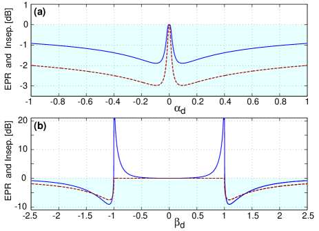
Figure 3: Harmonic entanglement observed in (a) SHG and (b) OPO. Both the EPR (solid lines) and the inseparability (dotted lines) entanglement measures are plotted as function of the fundamental and second harmonic field amplitudes, respectively.

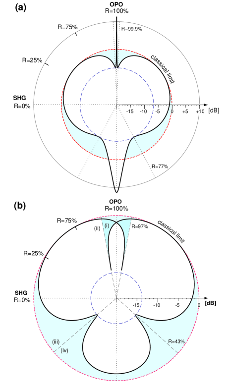
Figure 4: Polar plot of harmonic entanglement strength with a total input power of (a) 90% of threshold and (b) 400% of threshold. Shaded areas denote the presence of harmonic entanglement.

Results: Using these analytical results, we mapped out the degree of optimized EPR paradox ($\varepsilon_{o}$) of harmonic entanglement across the parameter space of fundamental and second-harmonic driving field amplitudes. This has been visualized in Fig. 2 where a greyscale-compatible color map has been assigned to a range of EPR values on a dB log (base 10) scale. Areas that are printed in dark ink, signify strong entanglement. White areas are not entangled, and are either at the standard quantum limit or greater (classical thermal states). The vertical $(\beta_{d})$ and horizontal $(\alpha_{d})$ axes of the plot coincide with the special cases of OPO and SHG respectively. Regions of interest have been individually labeled. Note that in order to represent bi-stability in the map, the left and right-hand sides of the map must be mentally folded along the OPO axis. The map of driving fields is clearly divided into the three distinct areas that correspond to the stable branches of the steady-state solutions. These are; (i) the bi-stable region above OPO threshold, (ii-iii) the mono-stable solution showing parametric amplification at (ii) and de-amplification at (iii). And finally, the so-called out-of-phase solution, which has a complex-valued fundamental field solution, is labeled with (iv). We find that the system produces a maximum entanglement of up to $\varepsilon_{o}=13.8~{}{\rm dB}$ at the intersection of (i-ii) and also when crossing (iii-iv). These regions correspond exactly to the critical boundaries where a branch change in the classical solution occurs.

A more detailed analysis of entanglement in SHG is shown in Fig. 3(a) where the EPR measure is plotted concomitant with the inseparability criterion as the amplitude of the driving field is varied. The strength of entanglement finds a maximum of $\varepsilon_{o}=1.9~{}{\rm dB}$ and $\mathcal{I}=3.0~{}{\rm dB}$ for the system driven with a fundamental field of $\alpha_{d}=\pm 0.1$. In SHG, entanglement is produced for all non-zero driving field amplitudes. However, the strength of the entanglement does not become arbitrarily high if loss in the system is made arbitrarily small. This is a bound set by the SHG process itself. Note that for a traveling-wave SHG process the strength of entanglement has been found to be $\varepsilon_{o}\approx 12~{}{\rm dB}$ WisemanOlsen . Contrast this behavior with the OPO process, which for below threshold, is not entangled, and only becomes entangled once the system is pushed beyond threshold. This is shown in Fig. 3(b). The maximum entanglement produced is $\varepsilon_{o}=9.1~{}{\rm dB}$ and $\mathcal{I}=7.5~{}{\rm dB}$ both for $\beta_{d}=\pm 1.1$. Note that as loss in the model is made arbitrarily small and for a driving field approaching OPO threshold, the entanglement becomes arbitrarily strong.

If we view the total input power to the system as a resource, then it is interesting to see how the strength of entanglement changes, as the power splitting ratio between the fundamental and second-harmonic field is varied, whilst keeping the total input power held constant. We define the splitting fraction to be $R=|\beta_{\rm 1,in}|^{2}/(\frac{1}{2}|\alpha_{\rm 1,in}|^{2}+|\beta_{\rm 1,in}|^{2})$, and follow a path, parameterized by angle $\theta_{R}$, as defined by $\alpha_{d}=(\beta_{1,{\rm in,c}}/\alpha_{1,{\rm in,c}})\sqrt{2\xi}\sin\theta_{R}$, and $\beta_{d}=\sqrt{\xi}\cos\theta_{R}$.

In Fig. 4 the total input power $\xi$ has been set to $90\%$ in (a) and $400\%$ in (b) of the power required to reach OPO threshold. A given angle in the plot describes not only the splitting fraction for fundamental and second-harmonic power, but also the relative phase between them ($0$ or $\pi$). The radial distance in the plot corresponds to the EPR measure of entanglement in a dB scale. A circle is drawn at $0~{}{\rm dB}$ to mark the classical limit. The shaded areas highlight the entanglement. We find that for a total input power required to reach $90\%$ OPO threshold, there is a choice of two splittings of $R=99.9\%$ and $R=77\%$, that both give a maximum amount of entanglement of $\varepsilon_{o}=6.5~{}{\rm dB}$ . These parameters correspond to neither a pure OPO, nor a pure SHG process, but correspond rather to an OPA operated in a moderately pump-depleted regime. In Fig. 4(b) we increase the resource available by setting the total input power to $400\%$ of OPO threshold. The bi-stability displayed by the system in region (i) is now clearly visible. As we drive the system from (i) through to region (ii), the entanglement approaches a strength of $\varepsilon_{o}=13.8~{}{\rm dB}$ at $R=97\%$. The same strength of entanglement is also found at $R=43\%$ which is exactly at the boundary between the regions (iii) and (iv). Arbitrarily strong entanglement can be produced in these boundary regions, provided that the system has sufficiently low loss, and is driven above threshold.

From these two examples, we can see that stronger entanglement is made available, when the system is driven by higher total input powers. This supports the view, that the total input power to the system is a resource for the generation of entanglement. To relate this result to a potential experimental demonstration, we stress that the amount of total input power needed to access at least $\varepsilon_{o}=6$ dB of entanglement is near to that required to reach threshold in OPO. Where both the detection of such entanglement, and the total input power required, are experimentally accessible Lam .

So far, we have only considered the case where the driving fields are coherent states. Although an in-depth discussion is contained in a forthcoming paper, we can qualitatively describe the effect that squeezed driving fields have on the harmonic entanglement generation for this system. In short, squeezing of the fundamental and/or the second-harmonic field in the correct combination of amplitude/phase quadratures, results not only in stronger entanglement, but also extends the regions of strong entanglement closer in toward the origin, thereby reducing the total input power needed to observe a given strength of entanglement.

Summary: We have shown that arbitrarily strong entanglement between a fundamental field and it’s second harmonic can, in principle, be generated by the second-order non-linear interaction. The maximal strength of this harmonic entanglement, as measured by the EPR and inseparability criteria, is produced neither by pure SHG, nor parametric oscillation, but rather by an intermediate process. We considered the total input power that drives the non-linear interaction as a resource for the strength of entanglement, and found that an experimental demonstration of harmonic entanglement using optical techniques should be attainable.

This research is supported by the Australian Research Council Discovery Grant scheme. W.P.B would like to acknowledge financial support from the Center for the Physics of Information, California Institute of Technology.

References

- (1) A. Aspect, P. Grangier, and G. Roger, Phys. Rev. Lett. 49, 91 (1982); Z. Y. Ou, S. F. Pereira, H. J. Kimble, and K. C. Peng, Phys. Rev. Lett. 68, 3663 (1992).
- (2) H. M. Wiseman, M. S. Taubman, and H. A. Bachor, Phys. Rev. A 51 3227 (1995); M. K. Olsen, Phys. Rev. A, 70, 035801 (2004).
- (3) L.-A. Wu, H. J. Kimble, J. L. Hall, and H. Wu, Phys. Rev. Lett. 57 2520 (1986).
- (4) P. K. Lam, T. C. Ralph, B. C. Buchler, D. E. McClelland, H.-A. Bachor, and J. Gao, J. Opt. B 1, 469 (1999).
- (5) T. C. Ralph, E. H. Huntington, Phys. Rev. A 66, 042321 (2002).
- (6) C. H. Bennett, G. Brassard, C. Crepeau, R. Jozsa, A. Peres, W. K. Wootters, Phys. Rev. Lett. 70, 1895 (1993).
- (7) A. M. Lance, T. Symul, W. P. Bowen, B. C. Sanders, and P. K. Lam, Phys. Rev. Lett. 92, 177903 (2004).
- (8) X. Li, Q. Pan, J. Jing, J. Zhang, C. Xie, K. Peng, Phys. Rev. Lett. 88, 047904 (2002).
- (9) W. P. Bowen, N. Treps, B. C. Buchler, R. Schnabel, T. C. Ralph, H.-A. Bachor, T. Symul, and P. K. Lam, Phys. Rev. A 67, 032302 (2003).
- (10) P. D. Drummond, K. J. McNeil, and D. F. Walls, Opt. Acta, 27, 321 (1980).
- (11) M. J. Collett and C. W. Gardiner, Phys. Rev. A 30, 1386 (1984).
- (12) L.-M. Duan, G. Giedke, J. I. Cirac, and P. Zoller, Phys. Rev. Lett. 84, 2722 (2000).
- (13) M. D. Reid and P. D. Drummond, Phys. Rev. Lett. 60, 2731 (1988); M. D. Reid, Phys. Rev. A, 40, 913 (1989).
- (14) W. P. Bowen, R. Schnabel, P. K. Lam, and T. C. Ralph, Phys. Rev. Lett. 90, 043601 (2003); W. P. Bowen, R. Schnabel, P. K. Lam, and T. C. Ralph, Phys. Rev. A 69, 012304 (2004).