Mesoscopic superposition and sub-Planck scale structure in molecular wave packets

Abstract

We demonstrate the possibility of realizing sub-Planck scale structures in the mesoscopic superposition of molecular wave packets involving vibrational levels. The time evolution of the wave packet, taken here as the SU(2) coherent state of the Morse potential describing hydrogen iodide molecule, produces cat-like states, responsible for the above phenomenon. We investigate the phase space dynamics of the coherent state through the Wigner function approach and identify the interference phenomena behind the sub-Planck scale structures. The optimal parameter ranges are specified for observing these features.

Mesoscopic superposition of coherent states and their generalizations, such as cat-like states, have attracted considerable attention in the recent literature schleich ; haroche ; tara , since they show a host of non-classical behaviors. In a remarkable paper, Zurek zurek demonstrated that appropriate superposition of some of these states with a classical action $A$ can lead to sub-Planck scale structures in phase space. These sub-Planck scale structures in the phase space are characterized by an area $\hbar^{2}/A$. Apart from their counter intuitive nature and theoretical significance, the above scale has been shown to control the effectiveness of decoherence, a subject of tremendous current interest in the area of quantum computation and information. Zurek’s realization made use of dynamical systems which exhibit chaotic behavior in the classical domain. Recently a cavity QED realization involving the mesoscopic superposition of the compass states have been given pathak . In principle, one could also use superpositions of cat-like states arising in quantum optical systems with large Kerr non-linearity tara .

In this paper, we demonstrate the possibility of realizing sub-Planck scale structures in the mesoscopic superposition of molecular wave packets, which involves vibrational levels. The time evolution of an initial wave packet, taken here as the SU(2) coherent state (CS) of the Morse potential produces cat-like states. These arise due to the quadratic dependence of the energy on the vibrational quantum number. The superposition of these states is responsible for the above phenomena. We study the spatio-temporal structure of these states, paying special attention to the fractional revival, which gives rise to four coherent states required for the observation of the sub-Planck structure. This structure can be clearly explained through the interference phenomena in phase space. For this, we investigate the phase space dynamics of the coherent state through the Wigner function approach and identify the optimal parameter ranges for a clear observation of these features.

Morse potential is well-known to capture the vibrational dynamics of a number of diatomic molecules vetchin1 ; vetchin2 ; morse ; dahl ; wolf . It is worth mentioning that the phenomena of revival and fractional revival averbukh ; bluhm ; robinett have been experimentally observed in wave packets involving vibrational levels stolow . Creation of the wave packets and observation of their dynamics are carried out through pump-probe method wilson . The control and analysis of molecular dynamics is achieved through ultrashort femto-second laser pulses garraway . Fractional revival can be probed by random-phase fluorescence interferometry warmuth . Recently, cat-like states, arising in the temporal evolution of the Morse system, have been proposed for use in the quantum logic operations shapiro1 .

Morse potential describing the vibrational motion of a diatomic molecule has the form

$$V(x)=D(e^{-2\beta x}-2e^{-\beta x})$$ (1)

where $x=r/r_{0}-1,\;r_{0}$ is the equilibrium value of the inter-nuclear distance $r$, $D$ is the dissociation energy and $\beta$ is a range parameter. We will be considering HI molecule, as an example, which has $30$ bound states, with $\beta=2.07932$, reduced mass $\mu=1819.99\;a.u.$, $r_{0}=3.04159\;a.u.$ and $D=0.1125\;a.u.$ Defining

$$\lambda=\sqrt{\frac{2\mu Dr^{2}_{0}}{\beta^{2}\hbar^{2}}}\;\;\mathrm{and}\;\;s=\sqrt{-\frac{8\mu r^{2}_{0}}{\beta^{2}\hbar^{2}}E},$$ (2)

eigen functions of the Morse potential can be written as

$$\psi_{n}^{\lambda}(\xi)=Ne^{-\xi/2}\xi^{s/2}L_{n}^{s}(\xi),$$ (3)

where $\xi=2\lambda e^{-\beta x};\;\;0<\xi<\infty$, and $n=0,1,...,[\lambda-1/2]$, with $[\rho]$ denoting the largest integer smaller than $\rho$, so that the total number of bound states is $[\lambda-1/2]$. The parameters $\lambda$ and $s$ satisfy the constraint condition $s+2n=2\lambda-1$.

Note that $\lambda$ is potential dependent, $s$ is related to energy $E$ and, by definition, $\lambda>0,\;s>0$. In Eq. (3), $L_{n}^{s}(y)$ is the associated Laguerre polynomial and N is the normalization constant:

$$N=\left[\frac{\beta(2\lambda-2n-1)\Gamma{(n+1)}}{\Gamma{(2\lambda-n)}r_{0}}\right]^{1/2}.$$ (4)

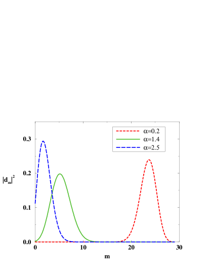
Figure 1: (Color online) $|d_{m}|^{2}$ plotted as a function of $m$ for the Morse potential of HI molecule for different values of $\alpha$.

Quite some time back, Nieto and Simmons gave a minimum uncertainty coherent state for Morse oscillator considering suitable conjugate variables nieto . Later, Benedict and Molnár benedict also found the same CS through super symmetric quantum mechanical method. This was used to describe the cat states of the NO molecule molnar . This CS involves infinite number of bound states, not belonging to the same potential charan . Morse potential has a finite number of bound states. Hence it is natural to expect an underlying SU(2) algebra. Recently, Dong et al., frank have obtained the SU(2) generators $\hat{J}_{+},\hat{J}_{-}$ and $\hat{J}_{0}$ which satisfy the algebra at the level of wave function as

$$\left[\hat{J}_{+},\hat{J}_{-}\right]\psi_{n}^{\lambda}(\xi)=2\hat{J}_{0}\psi_{n}^{\lambda}(\xi).$$ (5)

The SU(2) Perelomov coherent state of the Morse system is obtained by operating the displacement operator $e^{\alpha\hat{J}_{+}-\alpha^{*}\hat{J}_{-}}$ on the highest bound state $n^{\prime}$, defined by $\hat{J}_{+}\psi_{n^{\prime}}^{\lambda}(\xi)=0$. Using disentanglement theorem, the coherent state modulo normalization becomes

$$\chi(\xi) = e^{-\alpha\hat{J}_{-}}\psi_{n^{\prime}}^{\lambda}(\xi)$$ (6)

$$=\left[\psi_{n^{\prime}}^{\lambda}-\alpha\sqrt{n^{\prime}(s+n^{\prime}+1)}\;\psi_{n^{\prime}-1}^{\lambda}+...\right.$$

$$+\left.\frac{(-\alpha)^{n^{\prime}}}{({n^{\prime}})!}\sqrt{n^{\prime}!(s+n^{\prime}+1)(s+n^{\prime}+2)}\right.$$

$$\hskip 56.9055pt\left.\times\sqrt{....(s+2n^{\prime})}\;\;\psi_{0}^{\lambda}\right],$$

As is explicitly seen the above CS involves only the bound states, which are finite in number. This is due to the fact that the underlying group here is a compact group perelomov . For the purpose of our analysis, we consider this wave packet. We have checked that, superposition of Morse eigen states with suitable Gaussian weight factors, also reproduces the sub-Planck scale structure.

Simplifying the above expression, we can write it in a compact form:

$$\chi(\xi)=\sum_{m=0}^{n^{\prime}}d_{m}\;\psi_{m}^{\lambda}(\xi),$$ (7)

where

$$d_{m}=\frac{(-\alpha)^{n^{\prime}-m}}{(n^{\prime}-m)!}\left[\frac{n^{\prime}!\Gamma(2\lambda-m)}{m!\Gamma(2\lambda-n^{\prime})}\right]^{\frac{1}{2}}.$$ (8)

Fig. 1 shows $|d_{m}|^{2}$ distribution of HI molecule for various values of $\alpha$. For smaller values of $\alpha$, $|d_{m}|^{2}$ is peaked at higher values of $m$, where the anharmonicity is larger. The corresponding initial CS wave packet is not well localized and has an oscillatory tail. With the increase of $\alpha$, $|d_{m}|^{2}$ distribution moves towards the lower levels and the wave packet’s oscillatory tail gradually disappears. For larger values of $\alpha$, only the lower levels contribute to form the CS wave packet, where the effect of anharmonicity is rather small. Hence, it is clear that the choice of the distribution is quite crucial in the wave packet localization and its subsequent dynamics.

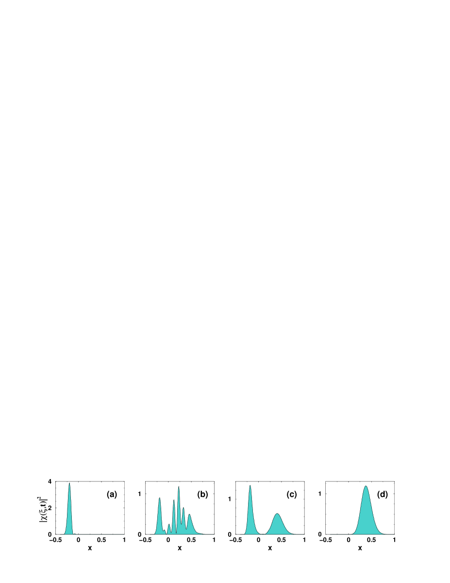
Figure 2: (Color online) Wave packet distribution in coordinate space for HI molecule, where $\alpha=1.4,\;\beta=2.07932$. Plotted here is $|\chi(\xi,t)|^{2}$ as a function of $x$ (where $\xi=2\lambda\exp[-\beta x])$ for (a) t=0, (b) $t=T_{\mathrm{rev}}/8$, (c) $t=T_{\mathrm{rev}}/4$ and (d) $t=T_{\mathrm{rev}}/2$.

Temporal evolution of CS state wave packet is given by

$$\chi(\xi,t)=\sum_{m}d_{m}\psi_{m}^{\lambda}(\xi)\exp[-iE_{m}t]$$ (9)

with $E_{m}=-(D/\lambda^{2})(\lambda-m-1/2)^{2}$. This quadratic energy spectrum yields classical and the revival times given by $T_{\mathrm{cl}}=T_{\mathrm{rev}}/(2\lambda-1)$ and $T_{\mathrm{rev}}=2\pi\lambda^{2}/D$ respectively. More interestingly, when $\mathrm{t}$ takes the values $\frac{r}{q}T_{\mathrm{rev}}$, where $r$ and $q$ are mutually prime integers, the CS wave packet can be written as a sum of classical CS wave packets averbukh :

$$\chi(\xi,t)=\sum_{p}^{l-1}a_{p}\;\chi_{\mathrm{cl}}[\xi,(r/q\;T_{\mathrm{rev}}-p/l\;T_{\mathrm{cl}})],$$ (10)

where

$$\chi_{\mathrm{cl}}(\xi,t)=\sum_{m}d_{m}\psi_{m}^{\lambda}(\xi)\exp[-2\pi imt/T_{\mathrm{cl}}].$$ (11)

Amplitudes are determined by

$$a_{p}=\frac{1}{l}\sum_{m}^{l-1}\exp\left[2\pi i(m^{2}r/q-mp/l)\right],$$ (12)

where $l=q/2$ when $q$ is an integer multiple of $4$ and $l=q$, in all other cases.

Fig. 2 shows the CS wave packet in the co-ordinate representation, where the revival behaviors at $T_{\mathrm{rev}}/4$ and $T_{\mathrm{rev}}/8$ are not transparent. We will now clarify the phase space picture of the wave packet at fractional revival times by using the Wigner function approach. We will also show that the interference phenomenon in phase space involving the cat-like states gives rise to the sub-Planck scale structure.

The Wigner function can be written as

$$W(x,p,t) = \frac{r_{0}}{\pi\hbar}\int_{-\infty}^{+\infty}\bar{\chi}^{*}(x-x^{\prime},t)$$ (13)

$$\times\bar{\chi}(x+x^{\prime},t)e^{-2ipx^{\prime}/\hbar}dx^{\prime}\;,$$

where $x$ is the scaled co-ordinate and $p$ is the corresponding scaled momentum and also $\bar{\chi}(x)=\chi(\xi)$.

Wigner functions at instances of fractional revival can be explained by making use of the decomposition of Eq. (10). At $t=T_{\mathrm{rev}}/8$, for example, the CS wave packet splits into four classical wave packets:

$$\chi(\xi,\frac{T_{\mathrm{rev}}}{8}) = \frac{1}{2}[e^{i\pi/4}\chi_{cl}(\xi,\frac{T_{\mathrm{rev}}}{8})$$ (14)

$$+ \chi_{cl}(\xi,\frac{T_{\mathrm{rev}}}{8}-\frac{T_{\mathrm{cl}}}{4})$$

$$- e^{i\pi/4}\chi_{cl}(\xi,\frac{T_{\mathrm{rev}}}{8}-\frac{T_{\mathrm{cl}}}{2})$$

$$+ \chi_{cl}(\xi,\frac{T_{\mathrm{rev}}}{8}-\frac{3T_{\mathrm{cl}}}{4})].\;$$

Defining

$$\chi^{\mathrm{(even,odd)}}_{\mathrm{cl}}(\xi,t)=\sum_{{\mathrm{m_{even,odd}}}}d_{m}\psi_{m}^{\lambda}(\xi)\exp[-2\pi im\frac{t}{T_{\mathrm{cl}}}]$$ (15)

expression Eq. (14) can be rewritten in a simpler form:

$$\chi(\xi,\frac{T_{\mathrm{rev}}}{8})=\chi^{\mathrm{even}}_{\mathrm{cl}}(\xi,\frac{T_{\mathrm{rev}}}{8}-\frac{T_{\mathrm{cl}}}{4})+e^{i\pi/4}\chi^{\mathrm{odd}}_{\mathrm{cl}}(\xi,\frac{T_{\mathrm{rev}}}{8}).$$ (16)

The above expression plays a crucial role in the explanation of the phase space behavior at $T_{\mathrm{rev}}/8$. Substituting this in Eq. (13), the Wigner function at $t=T_{\mathrm{rev}}/8$ can be written down as a sum of three terms: $W(x,p,T_{\mathrm{rev}}/8)=W^{(\mathrm{even})}+W^{(\mathrm{odd})}+W^{(\mathrm{int})}$, where $W^{(\mathrm{even})}$ and $W^{(\mathrm{odd})}$ are the Wigner functions corresponding to the first and second terms on the right hand side of Eq. (16) and $W^{(\mathrm{int})}$ is the contribution from the interference between these two terms. In Fig. 3, we have plotted $W(x,p,T_{\mathrm{rev}}/8)$ and its constituent parts for two values of $\alpha$. Note that both $W^{(\mathrm{even})}$ and $W^{(\mathrm{odd})}$ are Wigner functions of cat-like states. Each consists of two distinct peaks corresponding to two mesoscopic wave packets, and an oscillatory structure at the middle due to quantum interference between them. Furthermore, $W^{(\mathrm{even})}$ is along the east-west direction whereas $W^{(\mathrm{odd})}$ is along the north-south. This is because the time arguments of $\chi^{\mathrm{even}}_{\mathrm{cl}}$ and $\chi^{\mathrm{odd}}_{\mathrm{cl}}$ differ by $T_{\mathrm{cl}}/4$ in Eq. (16). The superposition of the interference regions of $W^{(\mathrm{even})}$ and $W^{(\mathrm{odd})}$ gives rise to the sub-Planck structure in Fig. 3(d). It is worth pointing out that $W^{\mathrm{int}}$, as plotted in Fig. 3(c), gives the off diagonal interferences of compass-like states produced at $T_{\mathrm{rev}}/8$.

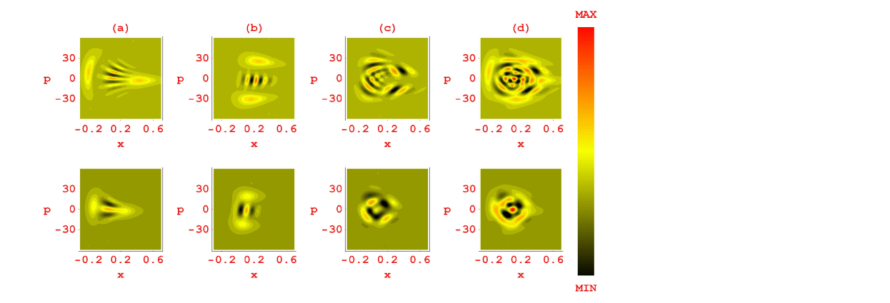
Figure 3: (Color online) The Wigner function $W(x,p,t)$ and its constituent parts at $t=T_{\mathrm{rev}}/8$ as a function of $x$ and $p$ for $\alpha=1.4$ (top row) and $\alpha=2.5$ (bottom row). Shown here are the contour plots of (a)$W^{(\mathrm{even})}$; (b)$W^{(\mathrm{odd})}$; (c)$W^{(\mathrm{int})}$ and (d)$W(x,p,t)$.

As seen in Fig. 1, for higher values of $\alpha$, the initial wave packet involves lower vibrational levels for which the turning points are nearer, resulting in a decrease in the span of the phase space variables. In this case, the area of overlap between the two interference structure increases and the number of ripples become less. As a consequence, the sub-Planck scale structure at the middle becomes more prominent as shown in the bottom array of Fig. 3. The four mini-wave packets, produced at $T_{\mathrm{rev}}/8$, are not equi-spaced and not of same size. The asymmetrical nature of the Morse potential is the main reason behind this. We also analyze numerically the expectation values of position and momentum at $t=T_{\mathrm{rev}}/8$ for different values of $\alpha$. The uncertainty product $(\triangle x\triangle p)$, obtained from this analysis, is $5.5914$ for $\alpha=1.4$ and $2.56404$ for $\alpha=2.5$ in the unit of $\hbar=1$. The classical action is defined by $A\approx\triangle x\triangle p$ and the corresponding dimension of the sub-Planck scale structure is $a\approx\hbar^{2}/A$ zurek , which easily comes out to be $0.179$ for $\alpha=1.4$ and $0.39$ for $\alpha=2.5$ respectively, implying the sub-Planck scale structure. Note that for smaller values of $\alpha$ the area becomes more sub-Planck.

In conclusion, we demonstrate that the interesting sub-Planck structure in mesoscopic quantum systems can indeed be realized in the temporal evolution of vibrational wave packets. This is clearly present, where four wave packets are produced in the temporal evolution. The coherence parameter $\alpha$ plays a crucial role in the formation of this structure; one needs the low-lying states for a clear observation of this structure. It is worth pointing out that, the vibrational wave packets are prone to decoherence through coupling to rotational and other vibrational levels. Recently methods like closed-loop control brif has been devised to minimize the decoherence effect.

References

- (1) W. Schleich and J. A. Wheeler, Nature 326, 574 (1987); W. Schleich and J. A. Wheeler, J. Opt. Soc. Am. B 4, 1715 (1987); W. Schleich, D. F. Walls, and J. A. Wheeler, Phys. Rev. A 38, 1177 (1988); W. P. Schleich, Quantum Optics in Phase Space (Wiley-VCH, Berlin, 2001) and references therein.
- (2) K. Tara, G. S. Agarwal, and S. Chaturvedi, Phys. Rev. A 47, 5024 (1993).
- (3) L. Davidovich, M. Brune, J. M. Raimond, and S. Haroche, Phys. Rev. A 53, 1295 (1996); J. M. Raimond, M. Brune, and S. Haroche, Phys. Rev. Lett. 79, 1964 (1997); A. Auffeves et al., ibid. 91, 230405 (2003).
- (4) W. H. Zurek, Nature 412, 712 (2001).
- (5) G. S. Agarwal and P. K. Pathak, Phys. Rev. A 70, 053813 (2004).
- (6) P. M. Morse, Phys. Rev. 34, 57 (1929).
- (7) S. I. Vetchinkin, A. S. Vetchinkin, V. V. Eryomin, and I. M. Umanskii, Chem. Phys. Lett. 215, 11 (1993).
- (8) S. I. Vetchinkin and V. V. Eryomin, Chem. Phys. Lett. 222, 394 (1994).
- (9) J. P. Dahl and M. Springborg, J. Chem. Phys. 88, 4535 (1988).
- (10) A. Frank, A. L. Rivera, and K. B. Wolf, Phys. Rev. A 61, 054102 (2000).
- (11) I. Sh. Averbukh and N. F. Perelman, Phys. Lett. A 139, 449 (1989).
- (12) R. Bluhm, V. A. Kostelecky, and J. Porter, Am. J. Phys. 64, 944 (1996).
- (13) R. W. Robinett, Phys. Rep. 392, 1 (2004) and references therein.
- (14) M. J. J. Vrakking, D. M. Villeneuve, and A. Stolow, Phys. Rev. A 54, R37 (1996).
- (15) J. Cao and K. R. Wilson, J. Chem. Phys. 106, 5062 (1997); A. H. Zewail, J. Phys. Chem. A. 104, 5660 (2000) and references therein.
- (16) B. M. Garraway and K.-A. Suominen, Contemp. Phys. 43, 97 (2002).
- (17) Ch. Warmuth, J. Chem. Phys. et al., 114, 9901 (2001).
- (18) E. A. Shapiro, M. Spanner, and M. Y. Ivanov, Phys. Rev. Lett. 91, 237901 (2003).
- (19) M. M. Nieto and L. M. Simmons, Jr., Phys. Rev. D 20, 1321 (1979).
- (20) M. G. Benedict and B. Molnár, Phys. Rev. A 60, R1737 (1999).
- (21) P. Földi, A. Czirják, B. Molnár, and M. G. Benedict, Opt. Exp. 10, 376 (2002).
- (22) T. Shreecharan, P. K. Panigrahi, and J. Banerji, Phys. Rev. A 69, 012102 (2004).
- (23) S. H. Dong, R. Lemus, and A. Frank, Int. J. Quant. Chem. 86, 433 (2002).
- (24) A. M. Perelomov, Generalized Coherent States and Their Applications (Springer, Berlin, 1986).
- (25) C. Brif, H. Rabitz, S. Wallentowitz, and I. A. Walmsley, Phys. Rev. A 63, 063404 (2001).