Two-Photon Entanglement in a Two-Mode Supersymmetric Model

Abstract

We will study entangled two-photon states generated from a two-mode supersymmetric model and quantify degree of entanglement in terms of the entropy of entanglement. The influences of the nonlinearity on the degree of entanglement is also examined, and it is shown that amount of entanglement increase with increasing the nonlinear coupling constant.

Keywords: Entanglement, Supersymmetry, Higgs algebra

PACS numbers: 03.67.-a, 03.67.Mn

1 Introduction

Perhaps, quantum entanglement is the most non-classical features of quantum mechanics which has recently attracted much attention although it was discovered many decades ago by Einstein, Podolsky, Rosen [1] and SchrÖdinger [2]. It plays a central role in quantum information theory and provides potential resources for communication and information processing [3, 4, 5]. By definition, a pure quantum state of two or more subsystems is said to be entangled if it is not a product of states of each components. A lot of works have been devoted to the preparation and measurement of entangled states. Moreover the possibility for generation of the entangled states with a fixed photon number has been theoretically studied [6, 7, 8, 9]. Duan et al described an entanglement purification protocol which generates maximally entangled states with fixed photon number from squeezed vacuum states or from mixed Gaussian continuous states by the quantum non-demolition measurement [6, 7]. Quantum teleportation using an entangled source of fixed photon number has also been theoretically investigated in [8]. Liu et al are used a system of two coupled microcrytallites as a source with fixed exciton number and quantified entanglement of the excitonic states [9]. Therefore, the generation of a new entangled source with fixed photon number is an interesting task both from experimental and theoretical viewpoints.

In this contribution, it is shown that a two-mode field with a two-photon interaction can be used as a good source for generation of entangled states with fixed photon number. We will study entangled states generated from two degenerate bosonic systems with fixed photon number, and we concern on quadratic nonlinearity between modes to use Higgs algebra as the spectrum generating algebra of the corresponding Hamiltonian [10, 11]. We also restrict ourselves to the case that total number of photons is odd. For this case, Debergh in [10] have shown that the corresponding Hamiltonian is supersymmetric [12].

A number of entanglement measures have been discussed in the literature, such as the von Neumann reduced entropy, the relative entropy of entanglement [13] and the so called entanglement of formation [5]. In order to discus entanglement of the states, we use von Neumann reduced entropy which has widely been accepted as an entanglement measure for pure bipartite states.

The organization of the paper is as follows. In section 2 we introduce a quantum optics model for two bosonic system with supersymmetric feature. An analyticl solution of the Hamiltonian is also given following the method of Ref. [10]. In section 3 the analytical results of section 2 are employed to generate entangled two-photon states with fixed photon number. Some examples are also considered in section 3. The paper is concluded in section 4 with a brief conclusion.

2 The two-mode supersymmetric Hamiltonian

In this section we shall introduce and analyse a model for nonlinear interaction between two-mode field. Our method is based on the analysis given in Ref. [10]. Let us consider the following family of Karrassiov-Klimov Hamiltonian [14] which describes multi-photon process of scattering, i.e.

$$H=\omega_{1}a_{1}^{\dagger}a_{1}+\omega_{2}a_{2}^{\dagger}a_{2}+g(a_{1}^{\dagger})^{s}a_{2}^{r}+g^{\ast}a_{1}^{s}(a_{2}^{\dagger})^{r}$$ (1)

where $0\leq r\leq s$, $g$ is coupling constant and $\omega_{i}\;(i=1,2)$ refer to angular frequencies of two-mode field characterized by annihilation and creation operators $a_{i}$, $a_{i}^{\dagger}$ respectively, satisfying $[a_{i},a_{j}^{\dagger}]=\delta_{ij}$. Hamiltonian (1) can be rewritten as

$$H=(\omega_{1}+\omega_{2})R_{0}+(s\omega_{1}-r\omega_{2})J_{0}+gJ_{+}+g^{\ast}J_{-},$$ (2)

where [11]

$$R_{0}\equiv\frac{1}{r+s}(ra_{1}^{\dagger}a_{1}+sa_{2}^{\dagger}a_{2}),$$ (3)

and

$$J_{0}\equiv\frac{1}{r+s}(a_{1}^{\dagger}a_{1}-a_{2}^{\dagger}a_{2}),\qquad J_{+}\equiv(a_{1}^{\dagger})^{s}a_{2}^{r},\qquad J_{-}\equiv a_{1}^{s}(a_{2}^{\dagger})^{r}.$$ (4)

It can be easily show that

$$[R_{0},J_{0}]=[R_{0},J_{\pm}]=0,$$ (5)

and

$$[J_{0},J_{\pm}]=\pm J_{\pm},$$ (6)

for arbitrary values of $r$ and $s$.

It is obvious that $R_{0}$ is a constant of motion, and the total photon number of the two-mode system is conserved. Moreover, the infinite dimensional vectors $\{|n_{1},n_{2}\rangle=\frac{(a_{1}^{\dagger})^{n_{1}}(a_{2}^{\dagger})^{n_{2}}}{\sqrt{n_{1}!n_{2}!}}|0,0\rangle$, $n_{1},n_{2}=0,1,2,\cdots\}$ are eigenvectors of $R_{0}$ with corresponding eigenvalues $j=\frac{rn_{1}+sn_{2}}{r+s}$. Debergh [10] has shown that in order to have Higgs algebra as the spectrum generating algebra of the Hamiltonian (2), we have to add to Eq. (6) the following requirement

$$[J_{+},J_{-}]=2J_{0}+8\beta J_{0}^{3},$$ (7)

and have shown that [10, 11] this is possible only for $r=s=2$, with parameter $\beta$ given by

$$\beta=-\frac{4}{4j^{2}+4j-2},\qquad j=0,\frac{1}{2},1,\cdots.$$ (8)

These values of $\beta$ lead to the relations [15]

$$J_{3}|j,m\rangle=\frac{m}{2}|j,m\rangle,$$ (9)

$$J_{\pm}|j,m\rangle=\sqrt{(j\mp m)(j\pm m+1)(j\mp m-1)(j\pm m+2)}|j,m\pm 2\rangle,$$ (10)

for $m=-j,-j+1\cdots,+j$. For a fixed total photon number $N$, the vectors $|j,m\rangle$ are related to the two-mode Fock states by

$$|j,m\rangle=|m_{1}\rangle_{A}|m_{2}\rangle_{B}=\frac{(a_{1}^{{\dagger}})^{j+m}(a_{2}^{{\dagger}})^{j-m}}{\sqrt{(j+m)!(j-m)!}}|0\rangle_{A}|0\rangle_{B},$$ (11)

where $|m_{1}\rangle_{A}\otimes|m_{2}\rangle_{B}$ represent Fock state with $m_{1}=j+m$ photons in mode A and $m_{2}=j-m$ photons in mode B.

In order to have more symmetry in Hamiltonian (2), let us suppose that $\omega_{1}=\omega_{2}=\omega$, and concern on the case that $g$ is real. In this case Hamiltonian (1) reduce to

$$\begin{array}[]{rl}H&=\omega(a_{1}^{\dagger}a_{1}+a_{2}^{\dagger}a_{2})+g\left((a_{1}^{\dagger})^{2}a_{2}^{2}+a_{1}^{2}(a_{2}^{\dagger})^{2}\right)\\ &=2\omega R_{0}+g\left(J_{+}+J_{-}\right).\end{array}$$ (12)

Now, by expanding eigenvectors of (12) as $|\psi_{k}\rangle=\sum_{m=-j}^{m=j}C_{m}^{(k)}|j,m\rangle$ and using eigenvalue equation $H|\psi_{k}\rangle=E_{k}|\psi_{k}\rangle$, we get

$$\begin{array}[]{rl}E_{k}C_{m}^{(k)}&=2j\omega C_{m}^{(k)}\\ &+gC_{m-2}^{(k)}\sqrt{(j+m)(j+m-1)(j-m+1)(j-m+2)}\\ &+gC_{m+2}^{(k)}\sqrt{(j-m)(j-m-1)(j+m+1)(j+m+2)}.\end{array}$$ (13)

Moreover in order to have supersymmetric Hamiltonian, Debergh concerned on the case that $j$ is a half-integer, which leads to twofold degeneracy of all eigenenergies as

$$E_{k}=2\omega j+g\lambda_{k},\qquad k=1,2,\cdots,j+\frac{1}{2},$$ (14)

where $\lambda_{k}$ is anyone of the $j+\frac{1}{2}$ different solutions of [10]

$$[F(A_{k},j,\lambda)]^{2}\equiv\left[\lambda^{j+\frac{1}{2}}-\sum_{k=1}^{j-\frac{1}{2}}A_{k}^{2}\lambda^{j-\frac{3}{2}}+\left(\sum_{k<l,\;|k-l|\neq 2}^{j-\frac{1}{2}}A_{k}^{2}A_{l}^{2}-A_{j-\frac{3}{2}}^{2}A_{j-\frac{1}{2}}^{2}\right)\lambda^{j-\frac{7}{2}}\right.$$

$$\left.-\left(\sum_{k<l<p,\;|k-l|\neq 2,\;|k-p|\neq 2,\;|l-p|\neq 2}^{j-\frac{1}{2}}A_{k}^{2}A_{l}^{2}A_{p}^{2}-\sum_{k=1}^{j-\frac{9}{2}}A_{k}^{2}A_{j-\frac{3}{2}}^{2}A_{j-\frac{1}{2}}^{2}\right)\lambda^{j-\frac{11}{2}}\cdots\right]^{2},$$ (15)

where $A_{k}$ are defined by

$$A_{k}=(k(k+1)(2j-k)(2j-k+1))^{\frac{1}{2}},\qquad k=1,2,\cdots,j-\frac{1}{2}.$$ (16)

Let us denote two eigenvectors of $H$ corresponding to twofold degenerate eigenvalue $E_{k}$ with $|\psi_{k}^{(1)}\rangle$ and $|\psi_{k}^{(2)}\rangle$. Now, since Eq. (13) relates coefficient $C_{m}^{(k)}$ to $C_{m+2}^{(k)}$ and $C_{m-2}^{(k)}$, we can, without lose of generality, write these two orthonormal eigenvectors belonging to eigensubspace $\varepsilon_{k}$ as

$$\begin{array}[]{ll}|\psi_{k}^{(1)}\rangle=\sum_{n=0}^{j-\frac{1}{2}}C_{j-2n}^{(k)}|j,j-2n\rangle,&C_{j-2n}^{(k)}=\frac{b_{j-2n}^{(k)}}{\sqrt{\sum_{n=0}^{j-\frac{1}{2}}\left(b_{j-2n}^{(k)}\right)^{2}}},\\ |\psi_{k}^{(2)}\rangle=\sum_{n=0}^{j-\frac{1}{2}}C_{j-2n-1}^{(k)}|j,j-2n-1\rangle,&C_{j-2n-1}^{(k)}=\frac{b_{j-2n-1}^{(k)}}{\sqrt{\sum_{n=0}^{j-\frac{1}{2}}\left(b_{j-2n-1}^{(k)}\right)^{2}}},\end{array}$$ (17)

where

$$\begin{array}[]{ll}b_{j}^{(k)}=1,&b_{j-2n}^{(k)}=\frac{F(A_{2p-1},n-\frac{1}{2},\lambda_{k})}{A_{1}A_{3}\cdots A_{2n-1}},\quad n=1,\cdots,j-\frac{1}{2},\\ b_{j-1}^{(k)}=1,&b_{j-2n-1}^{(k)}=\frac{F(A_{2p},n-\frac{1}{2},\lambda_{k})}{A_{2}A_{4}\cdots A_{2n}},\quad n=1,\cdots,j-\frac{1}{2},\end{array}$$ (18)

where function $F$ has been defined in Eq. (15). In two-mode Fock space representation, Eq. (17) can be written as

$$\begin{array}[]{l}|\psi_{k}^{(1)}\rangle=\sum_{n=0}^{\frac{2j-1}{2}}C_{j-2n}^{(k)}|2j-2n\rangle_{A}|2n\rangle_{B},\\ |\psi_{k}^{(2)}\rangle=\sum_{n=0}^{\frac{2j-1}{2}}C_{j-2n}^{(k)}|2j-2n-1\rangle_{A}|2n+1\rangle_{B}.\end{array}$$ (19)

Finally, evolution operator $U(t)$ takes the following form

$$U(t)=\sum_{k=1}^{j+\frac{1}{2}}e^{-iE_{k}t}\left(|\psi_{k}^{(1)}\rangle\langle\psi_{k}^{(1)}|+|\psi_{k}^{(2)}\rangle\langle\psi_{k}^{(2)}|\right).$$ (20)

3 Two-photon entanglement

In this section we will study entangled states generated by Hamiltonian (12). The entanglement measure that we are going to use is, the so called von Neumann entropy of reduced density matrix which has most widely been accepted as an entanglement measure of pure state of a bipartite system. Let $|\psi\rangle$ be a pure state of a bipartite system with state space $H_{A}\otimes H_{B}$. Entanglement of $|\psi\rangle$ is defined by

$$E(|\psi\rangle)=-\textmd{Tr}(\rho_{A}\textmd{ln}\rho_{A})=-\textmd{Tr}(\rho_{B}\textmd{ln}\rho_{B})=\sum_{n}\lambda_{n}^{2}\textmd{ln}\lambda_{n}^{2},$$ (21)

where $\rho_{A}$ is reduced density matrix of subsystem A which is obtained by tracing out subsystem B, i.e. $\rho_{A}=\textmd{Tr}_{B}(|\psi\rangle\langle\psi|)$, $\rho_{B}$ is defined similarly, and $\lambda_{n}$ are square root of nonzero eigenvalues of $\rho_{A}$ and $\rho_{B}$. They are also Schmidt number of state $|\psi\rangle$, i.e.

$$|\psi\rangle=\sum_{n}\lambda_{n}|u_{n}\rangle_{A}|v_{n}\rangle_{B},$$ (22)

where $\{|u_{n}\rangle\}$ and $\{|v_{n}\rangle\}$ are orthonormal states of two subsystems A and B, respectively. The definition is based on the fact that although entropy of a pure state is zero, but von Neumann entropy of each subsystem is zero only when the state $|\psi\rangle$ is a product state.

In this paper we shall consider the case that the total number of photons in the whole system is fixed by the initial condition $N=2j$, and system is initially in product state

$$|\psi(0)\rangle=|N-L\rangle_{A}|L\rangle_{B},$$ (23)

where represents initially $N-L$ photons in mode A and $L$ photons in mode B. By taking account of Eqs. (19), (20), (23), we obtain, up to an overall phase factor $e^{iN\omega}$, the final state of the system by

$$|\psi^{(N-L,L)}(t)\rangle=\sum_{n=0}^{\frac{N-1}{2}}a_{n}|N-2n-\Delta_{L}\rangle_{A}|2n+\Delta_{L}\rangle_{B},$$ (24)

where coefficients $a_{n}$ are defined by

$$a_{n}=\sum_{k=1}^{\frac{N+1}{2}}e^{-i\lambda_{k}t}\;C_{\frac{N}{2}-L}^{(k)}C_{\frac{N}{2}-2n-\Delta_{L}}^{(k)},$$ (25)

and $\Delta_{L}$ is difined such that it is zero (one) when $L$ is an even (odd) integer. Obviously, Eq. (24) represents final state of the system in Schmidt form and, accordingly, the von Neumann entropy of the reduced density matrix can be obtained easily by

$$E^{(N-L,L)}(t)=-\sum_{n=0}^{j-\frac{1}{2}}|a_{n}|^{2}\textmd{ln}|a_{n}|^{2}.$$ (26)

Finally, it should be stress that according to Eq. (26) maximal entangled state a of system with the total photon number $N$ is

$$|\psi_{MAX}^{(N)}\rangle=\frac{1}{\sqrt{N+1}}\sum_{n=0}^{N}|N-n\rangle_{A}|n\rangle_{B},$$ (27)

where in this case entropy of entanglement is equal to $E_{MAX}^{(N)}=\textmd{ln}(N+1)$. On the other hand, for state given by Eq. (24), maximum entropy of entanglement is obtained when $a_{n}=\sqrt{\frac{2}{N+1}}$, i.e.

$$|\psi_{MAX}^{(N-L,L)}\rangle=\sqrt{\frac{2}{N+1}}\sum_{n=0}^{\frac{N-1}{2}}|N-2n-\Delta_{L}\rangle_{A}|2n+\Delta_{L}\rangle_{B},$$ (28)

where we find $E_{MAX}^{(N-L,L)}=\textmd{ln}(\frac{N+1}{2})$. This means that for a system with fixed photon number $N$, maximum entanglement that can be achieved from Hamiltonian (12) is less than maximum entanglement that can be obtained from a system that linear interaction between modes is also considered. The difference between these two maximum is, of course, constant and equal to $\textmd{ln}(2)$.

In the rest of this section we will consider some examples in $N=1,3,5,9$ and discus results.

1. ${\mathbf{j}=\frac{1}{2}}$. In this case the total number of photons of system is $1$, and because of the twofold degeneracy of eigenvalues, the whole state space of system coincide with eigensubspace of the only eigenvalue. Accordingly the final state $|\psi(t)\rangle$ differs with initial product state only in a total phase factor, therefore, we can not have entanglement.

2. ${\mathbf{j}=\frac{3}{2}}$. In this case the state space of system decomposes into two eigensubspces, with eigenvalues

   $$E_{1}=3\omega+\sqrt{12}g\qquad E_{2}=3\omega-\sqrt{12}g.$$ (29)

   By starting with two initial states $|\psi(0)\rangle=|3\rangle_{A}|0\rangle_{B}$ and $|\psi(0)\rangle=|2\rangle_{A}|1\rangle_{B}$ we obtain, respectively

   $$|\psi^{(3,0)}(t)\rangle=\cos{(\sqrt{12}gt)}|3\rangle_{A}|0\rangle_{B}-i\sin{(\sqrt{12}gt)}|1\rangle_{A}|2\rangle_{B},\hskip 2.84526pt$$ (30)

   $$|\psi^{(2,1)}(t)\rangle=\cos{(\sqrt{12}gt)}|2\rangle_{A}|1\rangle_{B}-i\;\sin{(\sqrt{12}gt)}|0\rangle_{A}|3\rangle_{B}.$$ (31)

   By using Eq. (26), we obtain same value for entanglement of the above two states as

   $$\begin{array}[]{rl}E^{(3,0)}(t)&=E^{(2,1)}(t)\\ &=-\cos^{2}{(\sqrt{12}gt)}\;\textmd{ln}(\cos^{2}{(\sqrt{12}gt)})-\sin^{2}{(\sqrt{12}gt)}\;\textmd{ln}(\sin^{2}{(\sqrt{12}gt))}.\end{array}$$ (32)

   Equation (32) shows that entanglement has zero value when $t=\frac{k\pi}{2g}$ (for $k=0,1,\cdots$) and it takes maximum value $\textmd{ln}(2)$ at times $t=\frac{(2k+1)\pi}{4g}$ (for $k=0,1,\cdots$). This, obviously, shows that the survival time of maximum entanglement decrease with increasing of the nonlinear coupling constant $g$.

3. ${\mathbf{j}=\frac{5}{2}}$. This case corresponds with a system that has five photons and the state space of system decomposes into three eigensubspces, with eigenvalues

   $$E_{1}=5\omega\qquad E_{2}=5\omega+4\sqrt{7}g\qquad E_{3}=5\omega-4\sqrt{7}g.$$ (33)

   In this case by considering the initial state as anyone of $|\psi(0)\rangle=|5\rangle_{A}|0\rangle_{B}$, $|\psi(0)\rangle=|4\rangle_{A}|1\rangle_{B}$ and $|\psi(0)\rangle=|3\rangle_{A}|2\rangle_{B}$, we find, respectively, the final state of the system as

   $$\begin{array}[]{rl}|\psi^{(5,0)}(t)\rangle&=\frac{1}{14}\left(9+5\cos{(4\sqrt{7}gt)}\right)|5\rangle_{A}|0\rangle_{B}\\ &-i\sqrt{\frac{5}{14}}\sin{(4\sqrt{7}gt)}|3\rangle_{A}|2\rangle_{B}+\frac{3\sqrt{5}}{14}\left(-1+\cos{(4\sqrt{7}gt)}\right)|1\rangle_{A}|4\rangle_{B},\end{array}$$ (36)

   $$\begin{array}[]{rl}|\psi^{(4,1)}(t)\rangle&=\frac{1}{14}\left(5+9\cos{(4\sqrt{7}gt)}\right)|4\rangle_{A}|1\rangle_{B}\\ &-i\frac{3}{\sqrt{14}}\sin{(4\sqrt{7}gt)}|2\rangle_{A}|3\rangle_{B}+\frac{3\sqrt{5}}{14}\left(-1+\cos{(4\sqrt{7}gt)}\right)|0\rangle_{A}|5\rangle_{B},\end{array}\hskip 2.84526pt$$ (39)

   $$\begin{array}[]{rl}|\psi^{(3,2)}(t)\rangle&=-i\sqrt{\frac{5}{14}}\sin{(4\sqrt{7}gt)}|5\rangle_{A}|0\rangle_{B}\\ &+\cos{(4\sqrt{7}gt)}|3\rangle_{A}|2\rangle_{B}-i\frac{3}{\sqrt{14}}\sin{(4\sqrt{7}gt)}|1\rangle_{A}|4\rangle_{B}.\end{array}\hskip 56.9055pt$$ (42)

   

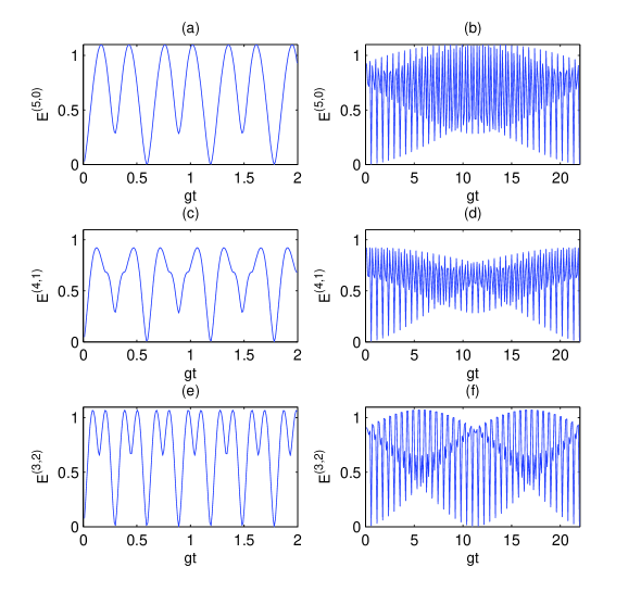
   Figure 1: $E^{(5,0)}$, $E^{(4,1)}$ and $E^{(3,2)}$ are plotted as a function of $gt$ in interval $[0,2]$ (curves $(a)$, $(c)$ and $(e)$) and in interval $[0,22.015]$ (curves $(b)$, $(d)$ and $(f)$).

   Figure (1) demonstrates the evolution of the entropy of entanglement as a function of $gt$ for three different initial states with different nonlinear coupling constant $g$. The figure is plotted such that the top horizontal line of each curve corresponds to the maximum entanglement $\textmd{ln}(3)$. The maximum entanglement that can be obtained by system is different for different initial state and the system can reach, approximately, to maximum entanglement $\textmd{ln}(3)$ only in the case that the initial state is $|\psi(0)\rangle=|5\rangle_{A}|0\rangle_{B}$. The Fig. (1) also shows that the survival time of maximum entanglement decrease when the difference between photon numbers of two modes A and B of the initial state is decreased. As the horizontal axis of the curves is product of coupling constant $g$ and time $t$, it is obvious that by increasing the nonlinear constant $g$, survival time of maximum entanglement decreases. Equations (36), (39) and (42) show that if the nonlinear coupling constant $g$ is equal to zero, then $|\psi(t)\rangle=|\psi(0)\rangle$, that is we can not have entangled state.

4. ${\mathbf{j}=\frac{9}{2}}$. Finally we consider as the last example the system with nine photons and accordingly the state space of system decomposes into five eigensubspces, with eigenvalues

   $$\begin{array}[]{ll}E_{1}=9\omega&\\ E_{2}=9\omega+\sqrt{792+24\sqrt{561}}g&E_{3}=9\omega+\sqrt{792-24\sqrt{561}}g\\ E_{4}=9\omega-\sqrt{792+24\sqrt{561}}g&E_{5}=9\omega-\sqrt{792-24\sqrt{561}}g.\end{array}$$ (43)

   

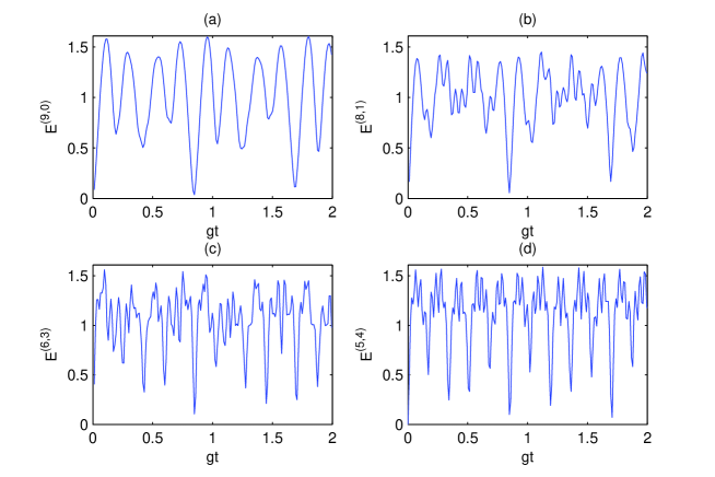
   Figure 2: $E^{(9,0)}$, $E^{(8,1)}$, $E^{(6,3)}$ and $E^{(5,4)}$ are plotted as a function of $gt$ (curves $(a)$, $(b)$, $(c)$ and $(d)$).

   The evolution of the entropy of entanglement as a function of $gt$ for four different initial states $|\psi(0)\rangle=|9\rangle_{A}|0\rangle_{B}$, $|\psi(0)\rangle=|8\rangle_{A}|1\rangle_{B}$, $|\psi(0)\rangle=|6\rangle_{A}|3\rangle_{B}$ and $|\psi(0)\rangle=|5\rangle_{A}|4\rangle_{B}$ is demonstrated in Fig. (2). The maximum entanglement that can be obtained by system is different for different initial states (the top horizontal line of each curve corresponds to the maximum entanglement $\textmd{ln}(5)$). We find that the maximum entanglement $\textmd{ln}(5)$ is obtained, approximately, only in the case that there are nine photons initially in one of the modes (for example mode A), i.e. $|\psi(0)\rangle=|9\rangle_{A}|0\rangle_{B}$. The survival time of the maximum entanglement decrease by increasing the nonlinear constant $g$ and it is also decrease by decreasing the difference between photon number of two modes A and B of the initial state.

4 Conclusion

We studied entangled states generated from two-mode supersymmetric model with fixed photon number. We found that only in the case that system has $N=3$ photons, the maximum entanglement can be obtained exactly. For other systems with total photon number greater than three, we found that the maximum entanglement is obtained, approximately, only in the case that all photons are initially in one of the modes, i.e. $|\psi(0)\rangle=|N\rangle_{A}|0\rangle_{B}$ or $|\psi(0)\rangle=|0\rangle_{A}|N\rangle_{B}$. The influences of the nonlinearity on the degree of entanglement is also examined, and is shown that survival time of maximum entanglement decrease by increasing the nonlinear coupling constant $g$. It is also shown that the survival time of maximum entanglement decreases when the difference between photon number of two modes A and B of the initial state is decreased.

Acknowledgments

This work was supported by the research department of university of Isfahan under Grant No. 831126.

References

[1] A. Einstein, B. Podolsky and N. Rosen,
Phys. Rev. 47, 777 (1935).
[2] E. SchrÖdinger, Naturwissenschaften
23, 807 (1935).
[3] C. H. Bennett, and S. J. Wiesner,
Phys. Rev. Lett. 69, 2881 (1992).
[4] C. H. Bennett, G. Brassard,
C. Crépeau, R. jozsa, A Peres and W. K. Wootters,
Phys.
Rev. Lett. 70, 1895 (1993).
[5] C. H. Bennett, D. P. DiVincenzo, J. A. Smolin and W.K.
Wootters, Phys. Rev. A 54, 3824 (1996).
[6] L. M. Duan, G. Giedke, J. I. Cirac and P. ZollerPhys. Rev. Lett.
84, 4002 (2000).
[7] L. M. Duan, G. Giedke, J. I. Cirac and P. ZollerPhys. Rev. A
62, 032304 (2000).
[8] P. T. Cochrane, G. J. Milburn and W. J. MunroPhys. Rev. A
62, 062307 (2000).
[9] Y-X Liu, S. K. Özdemir, A. Miranowicz, M. Koashi and N. Imoto
J. Phys. A: Math. Gen. 37, 4423 (2004).
[10] N. Debergh, J. Phys. A: Math. Gen.
31, 4013 (1998).
[11] J. Beckers, Y. Brihaye and N. Debergh, J. Phys. A: Math. Gen.
32, 2791 (1999).
[12] E. Witten, Nucl. Phys. B 188, 513 (1981).
[13] M. B. Plenio and V. Vedral, Phys. Rev. A
57, 1619 (1998).
[14] V. P. Karassiov and A. B. Klimov, Phys.
Lett. A 189, 43 (1994).
[15] N. Debergh, J. Phys. A: Math. Gen.
30, 5239 (1997).