Abstract

Quantum tomography is a procedure to determine the quantum state of a physical system, or equivalently, to estimate the expectation value of any operator. It consists in appropriately averaging the outcomes of the measurement results of different observables, obtained on identical copies of the same system. Alternatively, it consists in maximizing an appropriate likelihood function defined on the same data. The procedure can be also used to completely characterize an unknown apparatus. Here we focus on the electromagnetic field, where the tomographic observables are obtained from homodyne detection.

Chapter 0 Homodyne tomography and the reconstruction of quantum states of light

1 Introduction

The properties of each physical system are, by definition, completely determined by its quantum state. Its mathematical description is given in form of a density operator $\varrho$. Bohr’s principle of complementarity[1], which is in many ways connected with the uncertainty relations[2], forbids one to recover the quantum state from a single physical system. In fact, the precise knowledge of one property of the system implies that the measurement outcomes of the complementary observables are all equiprobable: the properties of a single system related to complementary observables are simultaneously unknowable. Moreover, the no-cloning principle[3] precludes to obtain many copies of a state starting from a single one, unless it is already known. Hence, complementarity and no-cloning prevent one to recover a complete information starting from a single quantum system, i.e. to recover its state. The only possibility is to recover it from multiple copies of the system. [Notice that, if the multiple copies are not all in the same quantum state, we will recover the mixed state of the ensemble]. Given $N$ copies of a system, we can either perform a collective measurement on all (or on subsets), or perform measurements separately on each system and combine the measurement results at the data analysis stage. Even though the former strategy would probably increase the speed of the statistical convergence of the measured state to the true one, it is quite impractical. Tomography thus adopts the latter strategy, which is the simplest to perform experimentally.

What is quantum tomography? It is the name under which all state reconstruction techniques are denoted. It derives from the fact that the first tomographic method (see Sec. 7) employed the same concepts of Radon-transform inversion we find in conventional medical tomographic imaging. Since then, better methods have evolved which eliminate the bias that the Radon-transform necessarily entails. These fall into two main categories: the plain averaging method and the maximum likelihood method. As will be seen in detail, the first method requires a simple averaging of a function calculated on the $N$ measurement outcomes $x_{n}$ of the homodyne quadratures $X_{\phi_{n}}$. Thus, the statistical error which affects the estimated quantity can be easily evaluated through the variance of the data. The second method, i.e. the maximum likelihood method, is based on the assumption that the data we obtained is the most probable. Hence, we need to search for the state that maximizes the probability of such data, i.e. the state $\varrho$ for which $\prod_{i=1}^{N}\;{}_{\phi_{n}}\!\langle x_{n}|\varrho|x_{n}\rangle_{\phi_{n}}$ is maximum, where ${}_{\phi_{n}}\!\langle x_{n}|\varrho|x_{n}\rangle_{\phi_{n}}$ is the probability of obtaining the result $x_{n}$ when measuring the quadrature $X_{\phi_{n}}$ (which has eigenstates $|x\rangle_{\phi_{n}}$).

Their involved mathematical derivation has given these tomographic techniques a false aura of being complicated procedures. This is totally unjustified: the reader only interested in applying the method can simply skip all the mathematical details and proceed to Sec. 5, where we present only the end result, i.e. the procedure needed in practice for a tomography experiment (the experimental setup is, instead, given in Sec. 1).

The chapter starts by introducing the method of homodyne tomography in Sec. 2, along with the description of homodyne detectors, noise deconvolution and adaptive techniques to reduce statistical errors. Then, in Sec. 3 we present the Monte Carlo integration methods and the statistical error calculations that are necessary for the plain averaging technique. In Sec. 4, the maximum likelihood methods are presented and analyzed. In Sec. 5, the step-by-step procedure to perform in practice a tomography experiment is presented. In Sec. 6, a tomographic method to calibrate (i.e. completely characterize) an unknown measurement device is presented. Finally, in Sec. 7, a historical excursus on the development of quantum tomography is briefly given.

2 Homodyne tomography

The method of homodyne tomography is a direct application of the fact that the displacements operators ${\cal D}(\alpha)=e^{\alpha a^{\dagger}-\alpha^{*}a}$ are a complete orthonormal set for the linear space of operators. Recalling that the scalar product in a space of operators takes the Hilbert-Schmidt form $\langle A|B\rangle=$Tr$[A^{\dagger}B]$, this means that

$$A=\int_{\mathbb{C}}\frac{d^{2}\alpha}{\pi}\;\mbox{Tr}[A\;{\cal D}^{\dagger}(\alpha)]{\cal D}(\alpha)=\int_{0}^{\pi}\frac{d\phi}{\pi}\int_{-\infty}^{+\infty}\!\!dr\frac{|r|}{4}\mbox{Tr}[A\;e^{irX_{\phi}}]e^{-irX_{\phi}}\;,$$ (1)

where the polar variables $\alpha\equiv-ir\;e^{i\phi}/2$ were used in the second equality. Upon introducing the probability $p(x,\phi)=\>_{\phi}\langle x|\varrho|x\rangle_{\phi}$ of obtaining $x$ when measuring the quadrature $X_{\phi}=(a^{\dagger}e^{i\phi}+ae^{-i\phi})/2$, one obtains the tomographic formula

$$\langle A\rangle=\hbox{Tr}[A\varrho]=\int_{0}^{\pi}\frac{d\phi}{\pi}\int_{-\infty}^{+\infty}dx\;p(x,\phi)\;K_{A}(x,\phi)\;,$$ (2)

where

$$K_{A}(x,\phi)\equiv\int_{-\infty}^{+\infty}dr\frac{|r|}{4}\mbox{Tr}[A\;e^{ir(X_{\phi}-x)}]\;,$$ (3)

defines the kernel of homodyne tomography. In the case of the density matrix reconstruction in the Fock basis $|n\rangle$ (i.e. when $A=|n\rangle\langle m|$), the kernel function is[4]

$$K_{A}(x,\phi) = 2e^{i(m-n)\phi}\sqrt{\frac{m!}{n!}}e^{-x^{2}}\sum_{j=m-n}^{n}\frac{(-1)^{j}}{j!}\left(\begin{array}[]{c}n\cr m-j\end{array}\right)\;$$

$$\times(2j+n-m+1)!\;\mbox{\sf Re}\Big{[}(-1)^{n-m}{\cal D}_{-2(2j+n-m+2)}(-2ix)\Big{]}\;,$$

where Re denotes the real part and ${\cal D}_{l}(x)$ denotes the parabolic cylinder function (which can be easily calculated through its recursion formulas).

The multimode case is immediately obtained by observing that the quadrature operators for different modes commute, so that for an operator $A_{M}$ (acting on the Hilbert space of $M$ modes) we find

$$\langle A_{M}\rangle=\int_{0}^{\pi}\frac{d\phi_{1}\cdots d\phi_{M}}{\pi^{M}}\int_{-\infty}^{+\infty}dx_{1}\cdots dx_{M}\;p(x_{1},\phi_{1},\cdots,x_{M},\phi_{M})$$

$$\qquad\qquad\times K_{A_{M}}(x_{1},\phi_{1},\cdots,x_{M},\phi_{M})\;,$$ (7)

where $p(x_{1},\phi_{1},\cdots,x_{M},\phi_{M})$ is the joint probability of obtaining the results $\{x_{m}\}$ when measuring the quadratures $\{X_{\phi_{m}}\}$, and where

$$K_{A_{M}}(x_{1},\phi_{1},\cdots)\equiv\int_{-\infty}^{+\infty}dr_{1}\cdots dr_{M}\prod_{m=1}^{M}\frac{|r_{m}|}{4}\mbox{Tr}[A_{M}\;e^{ir_{m}(X_{\phi_{m}}-x_{m})}]\;.$$ (8)

However, such a simple generalization to multimode fields requires a separate homodyne detector for each mode, which is unfeasible when the modes of the field are not spatio-temporally separated. This is the case, for example of pulsed fields, for which a general multimode tomographic method is especially needed, because of the problem of mode matching between the local oscillator and the detected fields (determined by their relative spatio-temporal overlap), which produces a dramatic reduction of the overall quantum efficiency. A general method for multimode homodyne tomography can be found[5] that uses a single local oscillator that randomly scans all possible linear combinations of incident modes.

1 Homodyne Detection

The balanced homodyne detector[6] measures the quadratures $X_{\phi}\equiv(a^{\dagger}e^{i\phi}+ae^{-i\phi})/2$. The experimental setup is described in Fig. 1. The input-output transformations of the modes $a$ and $b$ that impinge into a 50-50 beam-splitter are $c=(a+b)/\sqrt{2}$, $d=(a-b)/\sqrt{2}$ where $c$ and $d$ are the two beam-splitter output modes, each of which impinge into a different photodetector. The difference of the two photocurrents is the homodyne detector’s output, and thus is proportional to $c^{\dagger}c-d^{\dagger}d=a^{\dagger}b+b^{\dagger}a$. In the strong local oscillator limit, with mode $b$ in an excited coherent state $|\beta\rangle$ $(|\beta|\gg 1)$, the expectation value of the output is $I_{H}\propto\langle a^{\dagger}\rangle\beta+\langle a\rangle\beta^{*}$ which is proportional to the expectation value of the quadrature $X_{\phi}$, with $\phi$ the relative phase of the local oscillator.

file=homod.eps,width=2.in

Figure 1: Homodyne detector. The input signal (in mode $a$) is mixed by a 50-50 beam-splitter (BS) with a strong local oscillator (LO), which is coherent with the input field and is in a strong coherent state. The relative phase $\phi$ between the signal and the LO must be known and should be varied in $[0,\pi]$ with uniform probability. Two identical high efficiency linear photodetectors P₁ and P₂ measure the field. The photocurrents are then accurately subtracted electronically yielding the output $I_{H}$. Since the LO amplifies the weak quantum signals of the input, one can use high efficiency detectors that work only with strong signals.

A detector with non-unit quantum efficiency $\eta$ is equivalent[7] to a perfect $\eta=100\%$ detector, preceded by a beam-splitter with transmissivity $\eta$. Inserting two beam-splitters in front of the two photodiodes of the homodyne scheme, the modes $c$ and $d$ evolve as $c^{\prime}=\sqrt{\eta}\;c+\sqrt{1-\eta}\;u$ and $d^{\prime}=\sqrt{\eta}\;d+\sqrt{1-\eta}\;v$, where $u$ and $v$ are vacuum noise modes. The homodyne output, is now proportional to $c^{\prime{\dagger}}c^{\prime}-d^{\prime{\dagger}}d^{\prime}$, i.e. to $L\equiv\eta\;(a^{{\dagger}}b+b^{{\dagger}}a)+(1-\eta)(u^{{\dagger}}u-v^{{\dagger}}v)+\sqrt{{(1-\eta)\eta}/2}[a(u^{{\dagger}}-v^{{\dagger}})+b(u^{{\dagger}}+v^{{\dagger}})+a^{{\dagger}}(u-v)+b^{{\dagger}}(u+v)]$. As before, we take the limit $|\beta|\gg 1$ of strong pump in $b$, and rescale the output difference photocurrent by $2|\beta|\eta$, obtaining

$$I_{H}(\eta)=\lim_{|\beta|\to\infty}\frac{\langle L\rangle}{2|\beta|\eta}=\langle X_{\phi}\rangle+\sqrt{\frac{1-\eta}{2\eta}}\langle u_{\phi}+v_{\phi}\rangle\;,$$ (9)

where the modes $u$ and $v$ are in the vacuum state. Since the quadrature outcome for each vacuum state is Gaussian-distributed with variance $1/4$, this means that the distribution of the noisy data are a convolution of the clean data with a Gaussian of variance $\Delta_{\eta}^{2}=(1-\eta)/(4\eta)$, namely

$$p_{\eta}(x,\phi)=\frac{1}{\sqrt{2\pi\Delta^{2}_{\eta}}}\int_{-\infty}^{+\infty}dx^{\prime}e^{-(x-x^{\prime})^{2}/(2\Delta^{2}_{\eta})}\;p(x^{\prime},\phi)\;.$$ (10)

2 Noise deconvolution

The data-analysis procedure can be modified to yield the result we would obtain from perfect detectors, even though the data was collected with noisy ones[8]. In fact, depending on which operator $A$ we consider and on the value of the quantum efficiency $\eta$, the noise may be numerically deconvolved. The output of the noisy homodyne is distributed according to Eq. (10), and one can rewrite Eq. (2) as follows

$$\langle A\rangle=\int_{0}^{\pi}\frac{d\phi}{\pi}\int_{-\infty}^{\infty}dx\;p_{\eta}(x,\phi)\int_{-\infty}^{\infty}dr\;\frac{|r|}{4}\;e^{r^{2}\Delta_{\eta}^{2}/2}\;\mbox{Tr}[A\;e^{ir(X_{\phi}-x)}]\;,$$ (11)

where $p_{\eta}(x,\phi)$ is the probability of the noisy data. In the case when all the integrals are convergent, the noise inversion can be performed successfully.

It is clear the possibility of noise deconvolution depends on the quantum efficiency of the detectors and the operator to be estimated. For example, there is a bound $\eta>50\%$ for the reconstruction of the density matrix in the Fock basis (i.e. for $A=|n\rangle\langle m|$). In fact, one can see that for $\eta<50\%$ Eq. (11) has an unbounded kernel. Notice that actual homodyne detectors have efficiencies ranging between $70\%$ and $90\%$.

3 Adaptive tomography

Adaptive tomography[9] exploits the existence of null estimators to reduce statistical errors. In fact, the addition of a null estimator in the ideal case of infinite statistics does not change the average of the data since, by definition, the mean value of a null estimator is zero. However, it can change the variance of the data. Thus, one can look for a procedure to reduce the variance by adding suitable null functions.

In homodyne tomography null estimators are obtained as linear combinations of the following operators

$${\cal N}_{k,n}(X_{\varphi})=X_{\varphi}^{k}\,e^{\pm i(k+2+2n)\varphi}\;,\qquad k,n\geq 0\;.$$ (12)

One can easily check that such functions have zero average over $\varphi$, independently on $\varrho$. Hence, for every operator $A$ one actually has an equivalence class of infinitely many unbiased estimators, which differ by a linear combination of functions ${\cal N}_{k,n}(X_{\varphi})$. It is then possible to minimize the rms error in the equivalence class by the least-squares method. This yields an optimal estimator that is adapted to the particular set of experimental data. Examples of simulations of the adaptive technique that efficiently reduce statistical noise of homodyne tomographic reconstructions can be found in Ref. [9].

3 Monte Carlo methods for tomography

In this section we will very briefly review the basics of the Monte Carlo integration techniques that are needed and we show how to evaluate the statistical error bars of the tomographically estimated quantities.

A tomographic technique is based on an integral of the form

$$F=\int_{-\infty}^{+\infty}dx\,p(x)\,f(x)\;,$$ (13)

where $p(x)$ is a probability. Since we have experimental outcomes $\{x_{n},\ n=1,\cdots\,N\}$ distributed according to the probability $p(x)$, we sample the integral (13) using

$$\int_{-\infty}^{+\infty}dx\,p(x)\,f(x)=\lim_{N\to\infty}\frac{1}{N}\sum_{n=1}^{N}f(x_{n})\;.$$ (14)

For finite $N$, the sum will be an unbiased estimator for the integral, affected by statistical errors only (which can be made arbitrarily small by increasing $N$). The central limit theorem guarantees that the finite sum $F_{N}=\sum_{n=1}^{N}f(x_{n})/N$ is a statistical variable distributed as a Gaussian (for sufficiently high $N$) with mean value $F$ and variance

$$\sigma^{2}=\frac{1}{N^{2}}\sum_{n=1}^{N}\lim_{M\to\infty}\frac{1}{M}\sum_{j=1}^{M}\left[f(x_{j})\right]^{2}-F^{2}=\frac{\sigma^{2}(F)}{N}\;.$$ (15)

Hence, the tomographic estimated quantity converges with a statistical error that decreases as $1/{\sqrt{N}}$. It can be estimated from the data as

$$s^{2}(F_{n})=\frac{1}{N-1}\sum_{n=1}^{N}(F_{n}-m)^{2}\;.$$ (16)

[Remember that the factor $N-1$ in the variance denominator arises from the fact that we are using the experimental estimated mean value $m$ in place of the real one $F$.] The variance of the statistical variable ‘mean $m$’ is then given by $\sigma^{2}(m)=\sigma^{2}(F_{N})/N$, and thus the error bar on the mean $m$ estimated from the data is given by

$$\epsilon=\frac{1}{\sqrt{N}}\;s(F_{N})=\Big{[}\sum_{n=1}^{N}\frac{(F_{n}-m)^{2}}{N(N-1)}\Big{]}^{1/2}\;.$$ (17)

From the Gaussian integral one recovers the usual statistical interpretation to the obtained results: the “real” value $F$ is to be found in the interval $[m-\epsilon,m+\epsilon]$ with $\sim 68\%$ probability, in the interval $[m-2\epsilon,m+2\epsilon]$ with $\sim 95\%$ probability and in $[m-3\epsilon,m+3\epsilon]$ with $\sim$ unit probability.

In order to test that the confidence intervals are estimated correctly and that errors in the data analysis or systematic errors in the experimental data do not undermine the final result, one may check the $F_{n}$ distribution, to see if it actually is a Gaussian distribution. This can be done by comparing a histogram of the data to a Gaussian, or by using the $\chi^{2}$ test. Notice that when we have very low statistics it may be useful to use also bootstrapping techniques to calculate the variance of the data.

For a more rigorous treatment of the statistical properties of quantum tomography, and also some open statistical questions, see Ref. [10].

4 Maximum likelihood tomography

The maximum likelihood tomography is based on the assumption that the data obtained from the measurements is the most likely[11]. In contrast to the plain averaging method presented above, the outcome is not a simple average of functions of the data, but a Lagrange-multiplier maximization is usually involved. The additional complexity introduced is compensated by the fact that the results are statistically less noisy. Estimation of operator expectation values is, however, indirect: one must first estimate the state $\varrho$ and then calculate the expectation value as Tr$[\varrho A]$.

Consider a known probability distribution $p_{\gamma}(x)$ parametrized by a parameter $\gamma$ (which may also be a multidimensional parameter). We want to estimate the value of $\gamma$ from the data set $\{x_{1},\cdots,x_{N}\}$. The joint probability of obtaining such data is given by the likelihood function

$${\cal L}(x_{1},\cdots,x_{N};\gamma)=\prod_{i=1}^{N}p_{\gamma}(x_{k})\;.$$ (18)

The maximum likelihood procedure consists essentially in finding the $\gamma_{0}(x_{1},\cdots,x_{N})$ which maximizes the likelihood function ${\cal L}(x_{1},\cdots,x_{N};\gamma)$. Equivalently, it may be convenient to maximize its logarithm $\log{\cal L}(x_{1},\cdots,x_{N};\gamma)$, in order to convert into a sum the product in Eq. (18). Usually, various constraints are known on the parameters $\gamma$, which can be taken into account by performing a constrained maximization. The confidence interval for the estimated $\gamma_{0}$ can be evaluated from the data using a bootstrapping technique: we can extract a rough estimate of the probability distribution of the $\{x_{i}\}$ from the data set, generate $M$ simulated sets of $N$ data points, and repeat the procedure to obtain a set of $M$ parameters $\gamma_{0}^{(m)}$. Their variance estimates the variance of the reconstruction. Moreover, if a sufficiently large data set is present, we can attain the Cramer-Rao bound $\sigma_{\gamma}^{2}\geqslant 1/NF_{\gamma}$, where $F_{\gamma}$ is the Fisher information relative to $p_{\gamma}(x)$, i.e.

$$F_{\gamma}\equiv\int dx\frac{1}{p_{\gamma}(x)}\left(\frac{\partial}{\partial\gamma}\;p_{\gamma}(x)\right)^{2}\;.$$ (19)

Since the Cramer-Rao bound is achieved only for the optimal estimator[12], the maximum likelihood is among the best (i.e. least statistically noisy) estimation procedures.

The maximum likelihood method can be extended to the quantum domain[11]. The probability distribution of a measurement is given by the Born rule as $p_{i}=$Tr$[\Pi_{i}\varrho]$ where $\{\Pi_{i}\}$ is the positive operator-valued measurement (POVM) that describes the measurement. Thus we need to maximize the log-likelihood function $L(\varrho)\equiv\sum_{i}\log\;$Tr$[\Pi_{i}\varrho]$ over the set of density operators $\varrho$. In the case of finite Hilbert space, $L(\varrho)$ is a concave function defined on a convex set of density operators: its maximum is achieved on a single point or on a convex subset. The main difficulty of this procedure consists in finding a simple parameterization for the density matrix, that enforces both the positivity and the normalization Tr$[\varrho]=1$. The former is guaranteed by requiring that $\varrho=T^{\dagger}T$, the latter must be taken into account through an appropriate Lagrange multiplier. In order to employ the minimum number of parameters, it is sufficient to consider $T$ as an upper complex triangular matrix with nonnegative diagonal elements—so called Cholesky decomposition. This decomposition achieves minimal parameterization (up to the normalization condition), as it requires $d^{2}$ real parameters for a $d\times d$ Hermitian matrix. Thus, in practice we need to maximize the operator $L_{\lambda}[\varrho]\equiv\sum_{i}\log$Tr$[\Pi_{i}T^{\dagger}T]-\lambda[T^{\dagger}T]$, where $\lambda$ is a Lagrange multiplier that accounts for the normalization. By expressing $\varrho$ in terms of its eigenstates as $\varrho=\sum_{m}y^{2}_{m}|\psi_{m}\rangle\langle\psi_{m}|$, the condition for the maximum, $\partial L_{\lambda}/\partial y_{m}=0$, becomes

$$\sum_{i}\{y_{m}\langle\psi_{m}|\Pi_{i}|\psi_{m}\rangle/\mbox{Tr}[\varrho\Pi_{i}]\}-\lambda\;y_{m}=0\qquad\forall m\;.$$ (20)

Multiplying both members by $y_{m}$ and summing over $m$, through the Born rule and the normalization of $\varrho$, we find that $\lambda$ is equal to the number of measurements employed. Thus, we are left with the problem of finding the maximum of the $d^{2}$-parameter function $L_{\lambda=N}[\varrho=T^{\dagger}T]$, which can be tackled with conventional numerical techniques such as expectation-maximization or downhill simplex[11]. By using the ML method only small samples of data are required for a precise determination, even in the presence of low quantum efficiency at the detectors. However, we want to emphasize that such method is not always the optimal solution of the tomographic problem, since it suffers from some major limitations. Besides being biased due to the Hilbert space truncation—even though the bias can be very small if, from other methods, we know where to truncate—it cannot be generalized to the estimation of any ensemble average, but just of a set of parameters from which the density matrix depends. In addition, for the multi-mode case, the method has exponential complexity versus the number of modes.

5 Tomography for dummies

In this section we just give the step-by-step procedure to implement a tomography experiment, employing all the results obtained in the previous sections.

$\bullet$ Plain averaging method:

1. Calculate the Kernel function $K_{A}$ for the operator $A$ whose expectation value we want to estimate through Eq. (3). For example, to estimate the density matrix in the Fock basis, we need the $K_{A}$ defined in Eq. (2).

2. The experimental apparatus, described in Sec. 1, yields a set of $N$ data points $\{\phi_{n},x_{n}\}$ : each datum is composed by the quadrature phase $\phi_{n}$ that was measured and by the corresponding measurement result $x_{n}$ .

3. Evaluate $\frac{1}{N}\sum_{n}K_{A}(x_{n},\phi_{n})$. In the limit $N\to\infty$ this average yields the expectation value $\langle A\rangle$ we are looking for.

4. For finite $N$, we can estimate the purely statistical error on the result through Eq. (17), replacing $m$ with the average obtained at the previous point and $F_{n}$ with the $n$th Kernel function evaluation, $K_{A}[x_{n},X_{\phi_{n}})]$.

Further data massaging is also possible: we can employ adaptive tomography to reduce the statistical noise (see Sec 3). Moreover, we can remove the detector noise due to homodyne measurements with non unit quantum efficiency $\eta$, as long as $\eta>1/2$ (see Sec. 2).

$\bullet$ Maximum likelihood method:

1. Parametrize the unknown quantum state through the upper triangular $d\times d$ matrix $T$ as $\varrho=T^{\dagger}T$.

2. Use the same experimental apparatus (homodyne detection) to obtain $N$ data points $\{\phi_{n},x_{n}\}$. Calculate the log likelihood function on the experimental data as $\log\sum_{n=1}^{N}\;{}_{\phi_{n}}\!\langle x_{n}|T^{\dagger}T|x_{n}\rangle_{\phi_{n}}$.

3. Numerically maximize this quantity over the $d^{2}$ parameters of $T$ with the additional constrain Tr$[T^{\dagger}T]=1$. This maximum is achieved on our best estimate for the state $\varrho=T^{\dagger}T$.

4. The confidence intervals for our estimation can be obtained using bootstrapping techniques, or employing the Cramer-Rao bound of Eq. (19).

6 Quantum calibration of measurement devices

In this section we review the method to measure the POVM of an unknown measurement apparatus presented in Ref. [13]. The method is based on analyzing the correlations in measurements on a bipartite system: one of the two parts is fed into the unknown apparatus A, while the other is measured with a known set B of detectors that measures a quorum of observables (see Fig. 2). As will be shown in the following, there is ample freedom in the choice of both the input bipartite states and the set of observables. The procedure is repeated many times and the joint measurement outcomes are analyzed using the tomographic algorithms described above, which (in the limit of infinite input data) yield the POVM of the unknown apparatus. For finite data, the reconstructed POVM will be affected only by statistical errors which can be easily estimated. For the sake of illustration, a Monte-Carlo simulation of the procedure is given at the end of this section. It aptly illustrates the advantage of using maximum likelihood techniques over plain averaging: the maximum likelihood reconstruction is significantly less noisy.

file=experiment.eps,width=2.in          file=experimenth.eps,width=2.in

Figure 2: (Left) Experimental setup to determine the POVM of the unknown measurement apparatus A: one part of the bipartite input state $R$ is sent to the apparatus A which yields the measurement result $n$; the other part (with quantum state $\varrho_{n}$) is sent to the known detector B which performs a projective measurement of an observable $B_{k}$ from the complete set $\{B_{k}\}$ yielding the result $m(k)$. The joint measurement results are processed using a tomographic algorithm to obtain the POVM $\{\Pi_{n}\}$ of A. (Right) Example of application of the scheme to the radiation field. The bipartite state $R$ is generated via a non-linear crystal through spontaneous parametric down-conversion. The tomographer B is, in this case, a homodyne detector (HD) which measures the quadratures, a complete set of observables.

The following simple example illustrates how the procedure works. Suppose we want to evaluate the POVM of a von Neumann measurement of the observable $O$ which acts on a $d$-dimensional Hilbert space ${\cal H}_{A}$ and has spectral decomposition $\sum_{n}o_{n}|o_{n}\rangle\langle o_{n}|$. We can use the maximally entangled input state $|\Psi\rangle=\sum_{i=1}^{d}|i\rangle|i\rangle/\sqrt{d}$, which lives in the space ${\cal H}_{A}\otimes{\cal H}_{B}$. In fact, this state can be also written as

$$|\Psi\rangle=\frac{1}{\sqrt{d}}\sum_{i,j=1}^{d}\Big{(}|o_{j}\rangle\langle o_{j}|\otimes\leavevmode\hbox{\small 1\kern-3.0pt\normalsize 1}\Big{)}|i\rangle|i\rangle=\frac{1}{\sqrt{d}}\sum_{j=1}^{d}|o_{j}\rangle|o_{j}^{*}\rangle,$$ (21)

where $*$ denotes complex conjugation with respect to the basis $|i\rangle$. It is obvious from Eq. (21) that the outcome $o_{n}$ at detector A (corresponding to the state $|o_{n}\rangle$ in ${\cal H}_{A}$) means that the state $\varrho_{n}=|o_{n}^{*}\rangle\langle o_{n}^{*}|$ in ${\cal H}_{B}$ impinges in detector B. The POVM can be recovered using tomographical state reconstruction at B, since in this simple case $\Pi_{n}=\varrho^{*}_{n}$.

It is not difficult to generalize the above example to arbitrary POVMs and measurement procedures. Let the unknown apparatus A be described by the POVM $\{\Pi_{n}\}$ we want to estimate, and let the apparatus B measure the quorum observables $O_{k}$ described by the von Neumann projections $\{|k_{m}\rangle\langle k_{m}|\}$ (with $\{|k_{m}\rangle\}$ basis for all $k$). From the Born statistical formula we can derive the state that impinges into the known detector B if the unknown detector A gave result $n$ for the measurement on the initial bipartite state $R$, as

$$\varrho_{n}=\frac{\mbox{Tr}_{1}[(\Pi_{n}\otimes\leavevmode\hbox{\small 1\kern-3.0pt\normalsize 1})R]}{\mbox{Tr}[(\Pi_{n}\otimes\leavevmode\hbox{\small 1\kern-3.0pt\normalsize 1})R]}\;.$$ (22)

It describes the state reduction at B stemming from a measurement at A with outcome $n$. The denominator is the probability $p(n)$ of obtaining the result $n$ at B. The state $\varrho_{n}$ contains some information on the POVM element $\Pi_{n}$. It can be recovered by introducing the map ${\cal R}(X)\equiv\mbox{Tr}_{1}[(X\otimes\leavevmode\hbox{\small 1\kern-3.0pt\normalsize 1})R]$, so that Eq. (22) rewrites as $\varrho_{n}={\cal R}[\Pi_{n}/p(n)]$. This implies that the POVM can be recovered as $\Pi_{n}=p(n){\cal R}^{-1}(\varrho_{n})$, where the map $\cal R$ depends only on the input state $R$: the input state $R$ allows the POVM reconstruction if the inverse map ${\cal R}^{-1}$ exists. This condition can be cast in a more transparent form by rewriting the map $\cal R$ in a multiplicative form via isomorphism between operators on ${\cal H}\otimes{\cal H}$ and maps[14]. We can obtain an operator of this form by considering $S=R^{T_{1}}$, i.e. the partial transposition on the first space of the input state $R$. In fact, taking two operators $X$ and $Y$ such that $Y={\cal R}(X)$, we see that

$$Y_{il}=\sum_{jk}X_{jk}\langle i|{\cal R}\Big{(}|j\rangle\langle k|\Big{)}|l\rangle=\sum_{jk}X_{jk}(R^{T_{1}})_{jk,il}\;,$$ (23)

where $Y_{il}=\langle i|Y|l\rangle$, $X_{jk}=\langle j|X|k\rangle$, and $(R^{T_{1}})_{jk,il}=\langle j|\langle i|R^{T_{1}}|k\rangle|l\rangle$, the set $\{|n\rangle\}$ being a basis in $\cal H$. In matrix notation (considering $jk$ and $il$ as collective indexes), Eq. (23) rewrites as $Y=SX$. It follows immediately that the map $\cal R$ is invertible if $S^{-1}$ exists so that $X=S^{-1}Y$. In this case we say that the input state $R$ is faithful[14]. Since invertibility is a condition satisfied by a dense set of operators, the set of input states $R$ that allow the POVM reconstruction is also dense, i.e. almost any bipartite state will do. In particular, all Gaussian bipartite states—with the trivial exception of product states—are faithful [15]. To recapitulate: in order to check whether the state $\varrho_{n}$ allows to obtain the POVM (i.e. whether the input state $R$ is faithful) we must verify that the operator $(R^{T_{1}})_{jk,il}$ is invertible when $jk$ and $il$ are considered as collective indexes. As an illustration of this check, take the simple example given above: the state $|\Psi\rangle=\sum_{i}|ii\rangle/\sqrt{d}$ is faithful since $|\Psi\rangle\langle\Psi|^{T_{1}}=\sum_{ij}|ji\rangle\langle ij|/d$ is invertible: it is a multiple of the swap operator $E\equiv\sum_{ij}|ji\rangle\langle ij|$.

To recover $\varrho_{n}$ from the measurements at B (and hence the POVM if the input $R$ is faithful), we can use the quantum tomographic techniques described in the previous sections. If we employ the plain averaging technique, we may recover the density matrix elements $\varrho_{ij}$ in some basis and then calculate the POVM using the inverse map ${\cal R}^{-1}$, as

$$\langle j|\Pi_{n}|k\rangle=p(n)\sum_{il}\varrho^{(n)}_{il}\>(R^{T_{1}})^{-1}_{jk,il},$$

where the inverse of $R^{T_{1}}$ must be calculated considering $jk$ and $il$ as collective indexes. On the other hand, if we employ maximum likelihood we may directly maximize the probability of acquiring the data we obtained from the measurements[11], i.e. the joint probability $p_{k}(n,m)=$Tr$[(\Pi_{n}\otimes|k_{m}\rangle\langle k_{m}|)R]$. Equivalently, one can maximize the logarithm of this quantity and consider simultaneously all the $N$ joint measurement outcomes $\{n_{1},m_{1}\},\cdots,\{n_{N},m_{N}\}$ of the quorum operators $O_{k^{(i)}}$ at detector A and of the unknown detector B. Thus, the POVM $\{\Pi_{n}\}$ is the one that maximizes the quantity

$${\cal L}(\{\Pi_{n}\})\equiv\sum_{i=1}^{N}\log\mbox{Tr}\Big{[}(\Pi_{n_{i}}\otimes|k^{(i)}_{m_{i}}\rangle\langle k^{(i)}_{m_{i}}|)R\Big{]}\;,$$ (24)

with the additional constraints $\Pi_{n}\geqslant 0$ and $\sum_{n}\Pi_{n}=\leavevmode\hbox{\small 1\kern-3.0pt\normalsize 1}$. Other prior knowledge on the quantities to be estimated can be easily introduced adding further constraints to the maximization. Also in this case it is possible to take into account a known source of noise at the detector B: if we replace the term $|k^{(i)}_{m_{i}}\rangle\langle k^{(i)}_{m_{i}}|$ in Eq. (24) with the noise-evolved ${\cal N}(|k^{(i)}_{m_{i}}\rangle\langle k^{(i)}_{m_{i}}|)$, then the maximization yields the POVM that maximizes the noisy measurement results.

For the sake of illustration, we give a Monte-Carlo simulation of the calibration procedure in which we recover the POVM of a simple inefficient photodetector[13]. An inefficient photodetector is aptly modeled by a perfect photodetector (which is a device which measures the observable “number of photons” $a^{\dagger}a=\sum_{n}n|n\rangle\langle n|$), preceded by a beam-splitter with a transmissivity equal to the quantum efficiency $\eta$ of the detector. Possible dark counts can be considered by feeding the other beam-splitter port with a thermal state with $\bar{n}$ average photons. In this case, the theoretical POVM is given by

$$\Pi_{n}=\sum_{p=0}^{\infty}|p\rangle\langle p|\;$$ (25)

$$\times\sum_{k=0}^{\infty}\sum_{j=0}^{\min(p,k+n)}\left(\begin{array}[]{c}p\cr j\end{array}\right)\left(\begin{array}[]{c}-n-1\cr k\end{array}\right)\left(\begin{array}[]{c}k+n\cr j\end{array}\right)\eta^{j}(1-\eta)^{k+n-j}\;\bar{n}^{k+n-j}\;.$$ (32)

Since this POVM is diagonal in the Fock basis, we can limit the reconstruction to the diagonal elements. As input state $R$ we employ a twin beam state $|TB\rangle$, i.e. the result of spontaneous parametric down-conversion:

$$|TB\rangle\equiv\sqrt{1-|\xi|^{2}}\sum_{m}\xi^{m}|m\rangle_{a}|m\rangle_{b}\;,$$ (33)

where $\xi$ is the parametric amplifier gain and $|m\rangle_{a}$ and $|m\rangle_{b}$ are Fock states of the modes $a$ and $b$ that impinge in the detectors A and B respectively. This is a faithful state since $|TB\rangle\langle TB|^{T_{1}}=(1-|\xi|^{2})E\>\xi^{a^{\dagger}a}\otimes{\xi^{*}}^{b^{\dagger}b}$ (where $E$ is the swap operator) is invertible. The photon counter measures the mode $a$ at position A, while homodyne detection with quantum efficiency $\eta_{h}$ measures the mode $b$ at position B acting as tomographer (see Fig. 2). Since only the diagonal part of the POVM is needed, we can use a homodyne detector with uniformly distributed local oscillator phase. [A phase-controlled homodyne detector would allow to recover also the off-diagonal elements of the POVM, ensuring a complete characterization of the device.]

In Figs. 3 and 4 we present the results of the POVM reconstruction deriving from the two tomographic methods described above (simple averaging and maximum likelihood, respectively). The convergence of the maximum likelihood procedure is assured since the likelihood functional $\cal L$ is convex over the space of diagonal POVMs. However, the convergence speed can become very slow: in the simulation of Fig. 4 a mixture of sequential quadratic programming (to perform the constrained maximization) and expectation-maximization techniques were employed. From the graphs it is evident that the maximum likelihood estimation is statistically more efficient since it needs much less experimental data than tomography. This is a general characteristic of this method, since if the optimal estimator (i.e. the one achieving the Cramer-Rao bound) exists, then it is equal to the maximum likelihood estimator[11]. An added bonus, evident from Eq. (24), is that the maximum likelihood recovers all the POVM elements at the same time additionally increasing the statistical efficiency. On the other hand, the tomographic reconstruction is completely unbiased: no previous information on the quantity to be recovered is introduced.

This simulated experiment uses realistic parameters and is feasible in the lab with currently available technology[16]. The major experimental challenge lies in the phase matching of the detectors, i.e. in ensuring that the modes detected at A and B actually correspond to the modes $a$ and $b$ of the state $|TB\rangle$.

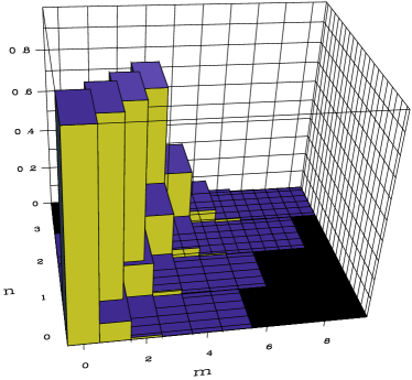
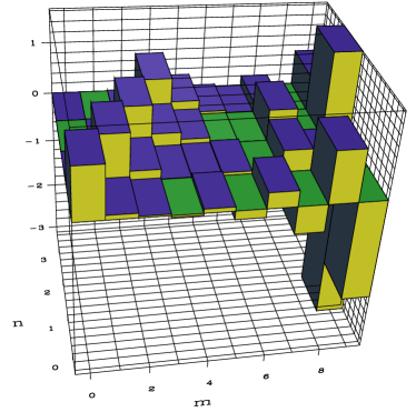
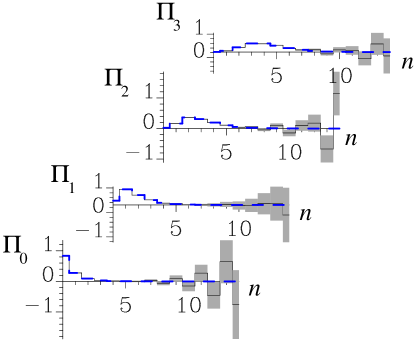
Figure 3: (Above left) Theoretical value of the diagonals of the POVM elements $\langle m|\Pi_{n}|m\rangle$ of the inefficient photodetector described by Eq. (25), with parameters $\bar{n}=1$, $\eta=80\%$. (Above right) Simulated reconstruction of the same quantity. The data are simulated as coming from an input twin-beam state $|TB\rangle$ with $\xi=0.88$, and as being detected from a phase insensitive homodyne detector with quantum efficiency $\eta_{h}=90\%$. Here $5\times 10^{6}$ simulated homodyne measurements are employed. (Below) The same data is plotted separately for each POVM element to emphasize the error bars. They are obtained from the root-mean-square of the recovered POVM matrix elements. (The theoretical value is plotted as the thick dashed line.) Plain tomographic averaging with noise deconvolution has been employed here, since the noise map of inefficient homodyne detection can be inverted for $\eta_{h}>50\%$.

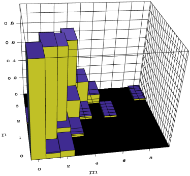
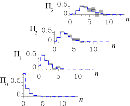
Figure 4: Maximum likelihood reconstruction of the same POVM of Fig. 3 with the same parameters, but here only $5\times 10^{4}$ simulated homodyne measurements are employed. The statistical error bars are obtained by bootstrapping, i.e. by calculating the variance using the data of $50$ numerical experiments. Notice that the result is statistically less noisy than the results presented in Fig. 3 even if here less measurements are employed: maximum likelihood is usually a better estimator.

7 History of quantum tomography

In this section a brief historical perspective (see also[17, 18]) on quantum tomography is presented. Already in 1957 Fano[19] stated the problem of quantum state measurement, followed by rather extensive theoretical work. It was only with the proposal by Vogel and Risken[20], however, that homodyne tomography was born. The first experiments followed[21] by showing reconstructions of coherent and squeezed states. The main idea at the basis of these works, is that it is possible to extend to the quantum domain the algorithms that are conventionally used in medical tomographic imaging to recover two-dimensional distributions (say of mass) from unidimensional projections in different directions. However, these first tomographic methods are unreliable for the measurement of unknown quantum states, since some arbitrary smoothing parameters have to be introduced.

A new approach to optical tomography was then proposed[22, 23] which allows to recover the quantum state of the field $\varrho$ (and also the mean values of system operators) directly from the data, abolishing all the sources of systematic errors. Only statistical errors (that can be reduced arbitrarily by collecting more experimental data) are left. Quantum tomography has been then generalized to the estimation of arbitrary observable of the field[24], to any number of modes[5], and to arbitrary quantum systems via group theory[25], with further improvements such as noise deconvolution[8], adaptive tomographic methods[9], and the use of max-likelihood strategies[11], which has made possible to reduce dramatically the number of experimental data, with negligible bias for most practical cases of interest. The latest developments are based on a general method[26], where the tomographic reconstruction is based on the existence of spanning sets of operators, of which group tomography[25] is just a special case.

Acknowledgments

We acknowledge financial support by INFM PRA-2002-CLON and MIUR for Cofinanziamento 2003 and ATESIT project IST-2000-29681.

References

- [1] N. Bohr, Naturwissenschaften 16, 245 (1928).
- [2] See, for example, S. Dürr and G. Rempe, Am. J. Phys. 68, 1021 (2000); O. Steuernagel, Eprint quant-ph/9908011 (1999).
- [3] W. K. Wootters and W. H. Zurek, Nature 299, 802 (1982); H. P. Yuen, Phys. Lett. A 113, 405 (1986).
- [4] G. M. D’Ariano, “Tomographic methods for universal estimation in quantum optics”, Scuola ’E. Fermi’ on Experimental Quantum Computation and Information, F. De Martini and C. Monroe eds. (IOS Press, Amsterdam 2002) pag. 385.
- [5] G. M. D’Ariano, P. Kumar, and M. F. Sacchi, Phys. Rev. A 61, 013806 (2000).
- [6] G. M. D’Ariano, “Quantum estimation theory and optical detection”, in Quantum Optics and the Spectroscopy of Solids, ed. by T. Hakioǧlu and A.S. Shumovsky, Kluwer Academic Publishers (1997), p. 139.
- [7] L. Mandel, Proc. Phys. Soc. 72, 1037 (1958); ibid. 74, 233 (1959); P. L. Kelley and W. H. Kleiner, Phys. Rev. A 30, 844 (1964).
- [8] G. M. D’Ariano, Phys. Lett. A 268, 151 (2000).
- [9] G. M. D’Ariano and M. G. A. Paris, Phys. Rev. A 60, 518 (1999); G. M. D’Ariano and M. G. A. Paris, Acta Phys. Slov. 48, 191 (1998).
- [10] L. M. Artiles, R. D. Gill, and M. I. Guta, J. Royal Stat. Soc. B 67, 109 (2005).
- [11] K. Banaszek, G. M. D’Ariano, M. G. A. Paris, and M. F. Sacchi, Phys. Rev. A 61, R10304 (2000).
- [12] H. Cramer, Mathematical Methods of Statistics (Princeton University Press, Princeton, 1946).
- [13] G. M. D’Ariano, P. Lo Presti, and L. Maccone, Phys. Rev. Lett. 93, 250407 (2004).
- [14] G. M. D’Ariano and P. Lo Presti, Phys. Rev. Lett. 86, 4195 (2001); 91, 47902 (2003).
- [15] G. M. D’Ariano and M. F. Sacchi, quant-ph 0503022.
- [16] See, for example: G. M. D’Ariano, M. Vasilyev, and P. Kumar Phys. Rev. A 58, 636 (1998); A. I. Lvovsky and S. A. Babichev, Phys. Rev. A 66, 011801R (2002); J. Wenger, R. Tualle-Brouri, and P. Grangier, Opt. Lett. 29, 1267 (2004); A. Zavatta, S. Viciani, and M. Bellini eprint quant-ph/0406090.
- [17] G. M. D’Ariano, “Measuring quantum states”, in Quantum Optics and the Spectroscopy of Solids, ed. by T. Hakioǧlu and A. S. Shumovsky, Kluwer Academic Publishers (1997), p. 175.
- [18] G. M. D’Ariano, M. G. A. Paris, and M. F. Sacchi, Quantum Tomography, Advances in Imaging and Electron Physics Vol. 128, p. 205 (2003); G. M. D’Ariano, M. G. A. Paris, and M. F. Sacchi, Quantum tomographic methods, in ”Quantum State Estimation”, Lecture Notes in Physics, vol. 649 (Springer-Verlag, Berlin, 2004) p. 7.
- [19] U. Fano, Rev. Mod. Phys. 29, 74 (1957), Sec. 6.
- [20] K. Vogel and H. Risken, Phys. Rev. A, 40, 2847 (1989).
- [21] D. T. Smithey, M. Beck, M. G. Raymer, and A. Faridani, Phys. Rev. Lett. 70, 1244 (1993); M. G. Raymer, M. Beck, and D. F. McAlister, Phys. Rev. Lett. 72,1137 (1994); D. T. Smithey, M. Beck, J. Cooper, and M. G. Raymer, Phys. Rev. A, 48, 3159 (1993).
- [22] G. M. D’Ariano, C. Macchiavello, and M. G. A. Paris, Phys. Rev. A 50, 4298 (1994).
- [23] G. M. D’Ariano, U. Leonhardt, and H. Paul, Phys. Rev. A 52, R1801 (1995).
- [24] G. M. D’Ariano, in Quantum Communication, Computing, and Measurement, ed. by O. Hirota, A. S. Holevo and C. M. Caves, Plenum Publishing (New York and London 1997), p. 253.
- [25] G. M. D’Ariano, in Quantum Communication, Computing, and Measurement, edited by P. Kumar, G. M. D’Ariano, and O. Hirota (Kluwer Academic/Plenum Publishers, New York and London, 2000), p. 137; G. Cassinelli, G. M. D’Ariano, E. De Vito, and A. Levrero, J. Math. Phys. 41, 7940 (2000); G. M. D’Ariano, L. Maccone, and M. Paini, J. Opt. B 5, 77 (2003).
- [26] G. M. D’Ariano, L. Maccone, and M. G. A. Paris, Phys. Lett. A 276, 25 (2000); J. Phys. A 34, 93 (2001).