Effect of noise and enhancement of nonlocality in on/off photodetection

Abstract

Nonlocality of two-mode states of light is addressed by means of CHSH inequality based on displaced on/off photodetection. Effects due to non-unit quantum efficiency and nonzero dark counts are taken into account. Nonlocality of both balanced and unbalanced superpositions of few photon-number states, as well as that of multiphoton twin beams, is investigated. We find that unbalanced superpositions show larger nonlocality than balanced one when noise affects the photodetection process. De-Gaussification by means of (inconclusive) photon subtraction is shown to enhance nonlocality of twin beams in the low energy regime. We also show that when the measurement is described by a POVM, rather than a set of projectors, the maximum achievable value of the Bell parameter in the CHSH inequality is decreased, and is no longer given by the Cirel’son bound.

I Introduction

Quantum entanglement for both discrete and continuous variable systems has been extensively analyzed, also revealing its subtle relations with other quantum mechanical features such as nonlocality. Indeed, it has been pointed out that the concept of entanglement coincides with nonlocality only for the simple case of bipartite pure states. As soon as we deal with mixed states, entangled states can be found which do not show properties of nonlocality while, not unexpectedly, the converse is always true wer89 . In addition, the amount of nonlocality, i.e., the amount of violation of a suitable Bell inequality, crucially depends on the nonlocality test adopted in the analysis, ranging from no violation to maximal violation for the same (entangled) quantum state.

In this paper we address nonlocality of different kinds of two-mode states of light by means of displaced on/off photodetection taking into account the effects of non-unit quantum efficiency and dark counts. This kind of measurement was first proposed in Ref. BW:PRL:99 , where, in particular, it was pointed out that the correlation functions violating the Bell inequalities (in the ideal case) involve the joint two-mode $Q$-function. The reason to pay a particular attention to on/off tests of nonlocality is twofold. On one hand, it has been shown that violation of Bell inequalities may be quite pronounced for some relevant state of light in the ideal case BW:PRL:99 . On the other hand, and more importantly, on/off tests may be effectively implemented with currently technology. In this framework, it is of interest to take into account the effects of experimental imperfections, e.g., non-unit quantum efficiency and nonzero dark counts bana:pra:02 , and to investigate the nonlocality properties of physically realizable entangled states. Indeed, realistic implementations of quantum information protocols require the investigation of nonlocality properties of quantum states in a noisy environment. In particular, the robustness of nonlocality should be addressed, as well as the design of protocols to preserve and possibly enhance nonlocality in the presence of noise.

The paper is structured as follows: in the next Section we describe in some detail the nonlocality test we use throughout the paper, while in Section III we analyze nonlocality of superpositions, both balanced (Bell states) and unbalanced, involving zero- and one-photon states. In Section IV we address the nonlocality of superpositions containing two-photon states, whereas Section V is focused on multiphoton twin-beam state. In Section VI we analyze the effect of dark counts on the violation of CHSH inequality, whereas in Section VII we address inconclusive photon subtraction (IPS) as a method to enhance nonlocality of twin-beam. Section VIII is devoted to a more detailed analysis of the choice of parametrization leading to violation of inequalities, whereas, in Section IX we show how a nonlocality test based on POVM measurement cannot yield the maximal violation of inequalities expressed by the Cirel’son bound. Finally, Section X closes the paper with some concluding remarks.

II Correlation functions and Bell parameter

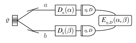
Figure 1: Scheme of the nonlocality test based on displaced on/off photodetection: the two modes $a$ and $b$ of a bipartite state $\varrho$ are locally displaced by an amount $\alpha$ and $\beta$ respectively, and then revealed through on/off photodetection. The corresponding correlation function violates Bell’s inequalities for dichotomous measurements for a suitable choice of the parameters $\alpha$ and $\beta$, depending on the kind of state under investigation. The violation holds also for non-unit quantum efficiency and non-zero dark counts.

The nonlocality test we are going to analyze is schematically depicted in Fig. 1: two modes of the radiation field, $a$ and $b$, are excited in a given (entangled) two-mode state described by the density matrix $\varrho$, and then are locally displaced by an amount $\alpha$ and $\beta$ respectively. Finally, the two modes are revealed by on/off photodetectors, i.e., detectors which have no output when no photon is detected and a fixed output when one or more photons are detected. The action of an on/off detector is described by the following two-value positive operator-valued measure (POVM) $\{\Pi_{0,\eta,D},\Pi_{1,\eta,D}\}$ FOP:2005

$${\Pi}_{0,\eta,D} =\frac{1}{1+D}\>\sum_{k=0}^{\infty}\left(1-\frac{\eta}{1+D}\right)^{k}|k\rangle\langle k|\>,$$ (1a)

$${\Pi}_{1,\eta,D} =\mathbb{I}-{\Pi}_{0,\eta,D}\>,$$ (1b)

$\eta$ being the quantum efficiency and $D$ the mean number of dark counts, i.e., of clicks with vacuum input. In writing Eq. (1) we have considered a thermal background as the origin of dark counts. An analogous expression may be written for a Poissonian background (see Appendix A). For small values of the mean number $D$ of dark counts (as it generally happens at optical frequencies) the two kinds of background are indistinguishable.

Overall, taking into account the displacement, the measurement on both modes $a$ and $b$ is described by the POVM (we are assuming the same quantum efficiency and dark counts for both the photodetectors)

$${\Pi}_{hk}^{(\eta,D)}(\alpha,\beta)={\Pi}_{h}^{(\eta,D)}(\alpha)\,\otimes{\Pi}_{k}^{(\eta,D)}(\beta)\,\;,$$ (2)

where $h,k=0,1$, and ${\Pi}_{h}^{(\eta,D)}(z)\equiv D(z)\,{\Pi}_{h,\eta,D}\,D^{{\dagger}}(z)$, $D(z)=\exp\left\{za^{\dagger}-z^{*}a\right\}$ being the displacement operator and $z\in{\mathbb{C}}$ a complex parameter.

In order to analyze the nonlocality of the state $\varrho$, we introduce the following correlation function:

$$E_{\eta,D}(\alpha,\beta) =\sum_{h,k=0}^{1}(-)^{h+k}\,\left\langle{\Pi}_{hk}^{(\eta,D)}(\alpha,\beta)\right\rangle$$ (3)

$$=1+4\,{\cal I}_{\eta,D}(\alpha,\beta)-2\,\left[{\cal G}_{\eta,D}(\alpha)+{\cal Y}_{\eta,D}(\beta)\right]\>,$$

where

$${\cal I}_{\eta,D}(\alpha,\beta)=\left\langle{\Pi}_{00}^{(\eta,D)}(\alpha,\beta)\right\rangle$$ (4a)

$${\cal G}_{\eta,D}(\alpha)=\left\langle{\Pi}_{0}^{(\eta,D)}(\alpha)\otimes\mathbb{I}\right\rangle$$ (4b)

$${\cal Y}_{\eta,D}(\beta)=\left\langle\mathbb{I}\otimes{\Pi}_{0}^{(\eta,D)}(\beta)\right\rangle\>,$$ (4c)

and where $\langle A\rangle\equiv{\rm Tr}[\varrho\,A]$ denotes ensemble average on both the modes. The so-called Bell parameter is defined by considering four different values of the complex displacement parameters as follows

$${\cal B}_{\eta,D}= \>\>E_{\eta,D}(\alpha,\beta)+E_{\eta,D}(\alpha^{\prime},\beta)+E_{\eta,D}(\alpha,\beta^{\prime})$$

$$-E_{\eta,D}(\alpha^{\prime},\beta^{\prime})$$ (5)

$$= \>\>2+4\left\{{\cal I}_{\eta,D}(\alpha,\beta)+{\cal I}_{\eta,D}(\alpha^{\prime},\beta)+{\cal I}_{\eta,D}(\alpha,\beta^{\prime})\right.$$

$$\left.-{\cal I}_{\eta,D}(\alpha^{\prime},\beta^{\prime})-{\cal G}_{\eta,D}(\alpha)-{\cal Y}_{\eta,D}(\beta)\right\}\,.$$ (6)

Any local theory implies that $|{\cal B}_{\eta,D}|$ satisfies the CHSH version of the Bell inequality, i.e., $|{\cal B}_{\eta,D}|\leq 2$ $\forall\alpha,\alpha^{\prime},\beta,\beta^{\prime}$ CHSH , while quantum mechanical description of the same kind of experiments does not impose this bound (see Section IX for more details on quantum-mechanical bounds on $|{\cal B}_{\eta,D}|$ in on/off experiments).

Notice that using Eqs. (1) and (4) we obtain the following scaling properties for the functions ${\cal I}_{\eta,D}(\alpha,\beta)$, ${\cal G}_{\eta,D}(\alpha)$ and ${\cal Y}_{\eta,D}(\beta)$

$${\cal I}_{\eta,D}(\alpha,\beta)=\left(\frac{1}{1+D}\right)^{2}\,{\cal I}_{\eta/(1+D)}(\alpha,\beta)$$ (7a)

$${\cal G}_{\eta,D}(\alpha)=\frac{1}{1+D}\,{\cal G}_{\eta/(1+D)}(\alpha)$$ (7b)

$${\cal Y}_{\eta,D}(\beta)=\frac{1}{1+D}\,{\cal Y}_{\eta/(1+D)}(\beta)$$ (7c)

where ${\cal I}_{\eta}={\cal I}_{\eta,0}$, ${\cal G}_{\eta}={\cal G}_{\eta,0}$, and ${\cal Y}_{\eta}={\cal Y}_{\eta,0}$. Therefore, it will be enough to study the Bell parameter for $D=0$, namely ${\cal B}_{\eta}={\cal B}_{\eta,0}$, and then we can use Eqs. (7) to take into account the effects of non negligible dark counts. From now on we will assume $D=0$ and suppress the explicit dependence on $D$. Notice that using expression (6) for the Bell parameter the CHSH inequality $|{\cal B}_{\eta,D}|\leq 2$ can be rewritten as

$$-1< \>\>{\cal I}_{\eta,D}(\alpha,\beta)+{\cal I}_{\eta,D}(\alpha^{\prime},\beta)+{\cal I}_{\eta,D}(\alpha,\beta^{\prime})$$

$$-{\cal I}_{\eta,D}(\alpha^{\prime},\beta^{\prime})-{\cal G}_{\eta,D}(\alpha)-{\cal Y}_{\eta,D}(\beta)<0\;,$$ (8)

which represents the CH version of the Bell inequality for our system CH .

In order to simplify the calculations, throughout this paper we will use the Wigner formalism. The Wigner functions associated with the elements of the POVM (1) for $D=0$ are given by (see Appendix A)

$$W[\Pi_{0,\eta}](z) = \frac{\Delta_{\eta}}{\pi\eta}\,\exp\left\{-\Delta_{\eta}\,|z|^{2}\right\}\,,$$ (9)

$$W[\Pi_{1,\eta}](z) = W[\mathbb{I}](z)-W[\Pi_{0,\eta}](z)\,,$$ (10)

with $\Delta_{\eta}=2\eta/(2-\eta)$, and $W[\mathbb{I}](z)=\pi^{-1}$. Then, noticing that for any operator $O$ one has

$$W[D(\alpha)\,O\,D^{{\dagger}}(\alpha)](z)=W[O](z-\alpha)\,,$$ (11)

it follows that $W[D(\alpha)\,{\Pi}_{0,\eta}\,D^{{\dagger}}(\alpha)](z)$ is given by

$$W[D(\alpha)\,{\Pi}_{0,\eta}\,D^{{\dagger}}(\alpha)](z)=W[\Pi_{0,\eta}](z-\alpha)\,,$$ (12)

and therefore

$$W[\Pi_{00}^{(\eta,0)}(\alpha,\beta)](z,w) =W[\Pi_{0,\eta}](z-\alpha)$$

$$\hskip 28.45274pt\times W[\Pi_{0,\eta}](w-\beta)$$ (13)

$$W[\Pi_{0,\eta}(\alpha)\otimes\mathbb{I}](z,w) =W[\Pi_{0,\eta}](z-\alpha)\>\pi^{-1}$$ (14)

$$W[\mathbb{I}\otimes\Pi_{0,\eta}(\beta)](z,w) =\pi^{-1}\>W[\Pi_{0,\eta}](w-\beta)\;.$$ (15)

Finally, thanks to the trace rule expressed in the phase space of two modes, i.e.,

$${\rm Tr}[O_{1}\,O_{2}]=\pi^{2}\int_{\mathbb{C}^{2}}\!d^{2}z\>d^{2}w\,W[O_{1}](z,w)\,W[O_{2}](z,w)\,,$$ (16)

one can evaluate the functions ${\cal I}_{\eta}(\alpha,\beta)$, ${\cal G}_{\eta}(\alpha)$, and ${\cal Y}_{\eta}(\beta)$, and in turn the Bell parameter ${\cal B}_{\eta}$ in Eq. (6), as a sum of Gaussian integrals in the complex plane.

III Nonlocality of the Bell states

We start our analysis by considering balanced superpositions of of zero- and one-photon states, i.e., the so-called Bell states, which are described by the density matrices

$$\varrho_{\pm}=|\Psi_{\pm}\rangle\langle\Psi_{\pm}|\,,\quad\sigma_{\pm}=|\Phi_{\pm}\rangle\langle\Phi_{\pm}|\,$$ (17)

where

$$|\Psi_{\pm}\rangle =\frac{1}{\sqrt{2}}\big{(}|1\rangle|0\rangle\pm|0\rangle|1\rangle\big{)}\,,$$ (18)

$$|\Phi_{\pm}\rangle =\frac{1}{\sqrt{2}}\big{(}|0\rangle|0\rangle\pm|1\rangle|1\rangle\big{)}\,.$$ (19)

In optical implementations Bell states $|\Psi_{\pm}\rangle$ are obtained from single-photon sources using linear optical elements, while preparation of $|\Phi_{\pm}\rangle$ requires active devices based on spontaneous parametric down-conversion.

The Wigner functions of the Bell states are given by

$$W[\varrho_{\pm}](z,w)= \>\>\frac{4}{\pi^{2}}\,\exp\left\{-2|z|^{2}-2|w|^{2}\right\}$$

$$\times\left(2\left|z\mp w\right|^{2}-1\right)\,,$$ (20)

and

$$W[\sigma_{\pm}](z,w)= \>\>\frac{4}{\pi^{2}}\,\exp\left\{-2|z|^{2}-2|w|^{2}\right\}$$

$$\times\left(1-2\left|z\mp w\right|^{2}+8\,|z|^{2}|w|^{2}\right)\,,$$ (21)

respectively.

Let us first consider $\varrho_{\pm}$. In this case the functions in Eqs. (4) are given by

$${\cal I}_{\eta}(\alpha,\beta)=\frac{1}{2}\,e^{-\eta(|\alpha|^{2}-|\beta|^{2})}\left[2(1-\eta)+\eta^{2}|\alpha\mp\beta|^{2}\right]$$ (22)

$${\cal G}_{\eta}(\alpha)={\cal Y}_{\eta}(\alpha)=\frac{1}{2}\,e^{-\eta|\alpha|^{2}}\left[2-\eta+\eta^{2}|\alpha|^{2}\right]\,,$$ (23)

while the Bell’s parameter is obtained using Eq. (6). Maximization of $|B_{\eta}|$, carried out using both analytical and numerical methods, indicates that the imaginary parts of the parameters $\alpha,\alpha^{\prime},\beta,\beta^{\prime}$ can be neglected for $\eta=1$, while it influences only slightly the value of $|B_{\eta}|$ for $\eta<1$. More details about the choice of the parametrization are given in Sec. VIII. Using the parameterizations: $\alpha=-\beta={\cal J}$, $\alpha^{\prime}=-\beta^{\prime}=-\sqrt{11}{\cal J}$ for the state $|\Psi_{+}\rangle$, and $\alpha=\beta={\cal J}$, $\alpha^{\prime}=\beta^{\prime}=-\sqrt{11}{\cal J}$ for the state $|\Psi_{-}\rangle$ with ${\cal J}\in{\mathbb{R}}$ we get the same Bell’s parameter for both the states and a maximum violation $|B|=2.68$ (when $\eta=1$). The Bell’s parameter for $\varrho_{\pm}$ is shown in Fig. 2 (a) as a function of ${\cal J}$ and $\eta$.

If we consider $\sigma_{\pm}$, we have

$${\cal I}_{\eta}(\alpha,\beta)= \frac{1}{2}\,e^{-\eta(|\alpha|^{2}+|\beta|^{2})}\,\big{\{}2(1-\eta)+\eta^{2}\big{[}1+|\alpha\pm\beta^{*}|^{2}$$

$$+(1-\eta|\alpha|^{2})(1-\eta|\beta|^{2})\big{]}\big{\}}\,,$$ (24)

whereas ${\cal G}_{\eta}(\alpha)$ and ${\cal Y}_{\eta}(\beta)$ are given in Eq. (23). As for the states $|\Psi_{\pm}\rangle$, the optimal parametrization has been obtained by a semi-analytical analysis. We get $\alpha=-\beta={\cal J}$, $\alpha^{\prime}=-\beta^{\prime}=-\sqrt{11}{\cal J}$ for the state $|\Phi_{+}\rangle$, and $\alpha=\beta={\cal J}$, $\alpha^{\prime}=\beta^{\prime}=-\sqrt{11}{\cal J}$ for the state $|\Phi_{-}\rangle$ (see Sec. VIII for more details). Thanks to this choice, ${\cal B}_{\eta}$ is maximized (when $\eta=1$) for both the Bell states $\sigma_{\pm}$. The results are shown in Fig. 2 (b).

The overall effect of non-unit quantum efficiency is to reduce the interval of ${\cal J}$ values in which there is violation. Notice that the states $|\Phi_{\pm}\rangle$ are slightly more robust than the $|\Psi_{\pm}\rangle$ one. In fact, one has $|{\cal B}_{\eta}|\leq 2$. as far as $\eta$ falls below $83.6\%$ for $|\Psi_{\pm}\rangle$ and $81.6\%$ for $|\Phi_{\pm}\rangle$. These results are consistent with the study given in Ref. bana:pra:02 , where the authors also have taken into account mode mismatch and have used a numerical algorithm in order to find the best choice of the parameters $\alpha$, $\beta$, $\alpha^{\prime}$, and $\beta^{\prime}$.

III.1 Unbalanced superpositions

Our analysis of on-off photodetection is aimed to describe optical implementations of nonlocality tests, where most of the experiments have been realized. In this framework the Bell states $|\Psi_{\pm}\rangle$ may be obtained from single-photon sources using balanced beam-splitters. In order to take into account possible imperfections it is worth to analyze nonlocality properties of the class of states that can be obtained from unbalanced beam splitters. Indeed, the analysis given above can be extended in order to describe general superpositions of the form

$$|\Psi_{\varphi}\rangle =\sin\varphi|1\rangle|0\rangle+\cos\varphi|0\rangle|1\rangle\,,$$ (25)

$$|\Phi_{\varphi}\rangle =\sin\varphi|0\rangle|0\rangle+\cos\varphi|1\rangle|1\rangle\,.$$ (26)

Since the calculations are similar to the ones of the Bell states, here we do not explicitly write the analytical results for the states $|\Psi_{\varphi}\rangle$ and $|\Phi_{\varphi}\rangle$. Rather, we plot the corresponding Bell parameter ${\cal B}_{\eta}$ in Figs. 3 and 4. In both the plots we used the same parametrization as for the Bell states. As one can see in Fig. 3, in the case of the superposition $|\Psi_{\varphi}\rangle$ the best result are obtained for the balanced superposition, namely $\varphi=\pi/4$. On the other hand, the case of $|\Phi_{\varphi}\rangle$ shows a different behavior: here the maximum of the violation for the ideal case (i. e. $\eta=1$) is achieved for a value of $\varphi$ slightly smaller than $\pi/4$, and it increases as the detection efficiency decreases. Moreover, by the comparison between Fig. 2 (b) and Fig. 3, we can see that, for the particular choice of the parametrization, when $\eta=0.8$ the balanced superposition does not violates the CHSH inequality, whereas, adjusting the parameter $\varphi$, the unbalanced superposition violates it and it does until the efficiency falls below the threshold value $\eta\approx 0.74$.

IV Nonlocality of superpositions containing two-photon states

A two-photon state which can be easily produced is the one obtained when two single-photon states impinge simultaneously in a balanced beam splitter: in this case the output state is given by

$$|\Omega\rangle=\frac{1}{\sqrt{2}}\big{(}|2\rangle|0\rangle+|0\rangle|2\rangle\big{)}$$ (27)

and the corresponding Wigner function reads as follows:

$$W[\Omega](z,w)= \>\>\frac{4}{\pi^{2}}\,\exp\left\{-2|z|^{2}-2|w|^{2}\right\}$$

$$\times\Big{[}1-4\Big{(}|z|^{2}+|w|^{2}-\big{|}z^{2}-{w^{*}}^{2}\big{|}^{2}\Big{)}\Big{]}\,,$$ (28)

Now, the functions defined in Eqs. (4) are given by

$${\cal I}_{\eta}(\alpha,\beta)= e^{-\eta(|\alpha|^{2}-|\beta|^{2})}$$

$$\times\Bigg{\{}(1-\eta)\big{[}1-\eta+\eta^{2}\big{(}|\alpha|^{2}+|\beta|^{2}\big{)}\big{]}$$

$$\hskip 42.67912pt-\frac{\eta^{4}}{4}\big{|}\alpha^{2}-{\beta^{*}}^{2}\big{|}^{2}\Bigg{\}}\,,$$ (29)

$${\cal G}_{\eta}(\alpha)= {\cal Y}_{\eta}(\alpha)=e^{-\eta|\alpha|^{2}}\,\Bigg{[}1-\eta+\frac{\eta^{2}}{2}$$

$$\hskip 42.67912pt+\eta^{2}(1-\eta)|\alpha|^{2}+\frac{\eta^{4}}{4}|\alpha|^{4}\Bigg{]}\,.$$ (30)

The parametrization which maximizes the violation of the inequality $|{\cal B}_{\eta}|\leq 2$ is $\alpha=\beta=0$ and $\alpha^{\prime}={\beta^{\prime}}^{*}=\sqrt{2}\,e^{i\pi/4}{\cal J}$ and, as for the Bell states, has been obtained by means of a semi-analytical analysis. As it is apparent from Fig. 5, in this case the violation is quite smaller than the previous ones: the maximum violation ${\cal B}_{\eta}=-2.07$ is achieved when ${\cal J}=0.45$ and $\eta=1$. Also the threshold for violation on the quantum efficiency is higher: for $\eta<92\%$ we have $|{\cal B}_{\eta}|<2$.

V Nonlocality of the twin beam

The twin-beam state (TWB) of radiation

$$|r\rangle=\frac{1}{\sqrt{\cosh r}}\sum_{n=0}^{\infty}\tanh^{n}r\>|n\rangle\otimes|n\rangle$$

may be produced by spontaneous downconversion in a nonlinear crystal. TWB is described by the Wigner function

$$W_{r}(z,w)=\frac{4}{\pi^{2}}\exp\{- 2A(|z|^{2}+|w|^{2})$$

$$+2B(zw+z^{*}w^{*})\}\,,$$ (31)

with $A\equiv A(r)=\cosh(2r)$ and $B\equiv B(r)=\sinh(2r)$, $r$ being the so-called squeezing parameter of the TWB. Since $W_{r}$ and the Wigner functions of the POVM (2) are Gaussian, it is quite simple to evaluate ${\cal I}_{\eta}(\alpha,\beta)$, ${\cal G}_{\eta}(\alpha)$, and ${\cal Y}_{\eta}(\beta)$ of the correlation function (3) and, then, ${\cal B}_{\eta}$; we have

$${\cal I}_{\eta}(\alpha,\beta)=\frac{4{\cal M}_{\eta}(r)}{\eta^{2}}\,\exp\big{\{}- \widetilde{F}_{\eta}\,(|\alpha|^{2}+|\beta|^{2})$$

$$+\widetilde{H}_{\eta}\,(\alpha\beta+\alpha^{*}\beta^{*})\big{\}}$$ (32)

with

$$\widetilde{F}_{\eta}\equiv\widetilde{F}_{\eta}(r)=\Delta_{\eta}-(2A+\Delta_{\eta})\,{\cal M}_{\eta}(r)$$ (33)

$$\widetilde{H}_{\eta}\equiv\widetilde{H}_{\eta}(r)=2B{\cal M}_{\eta}(r)$$ (34)

$${\cal M}_{\eta}(r)=\frac{\Delta_{\eta}^{2}}{4(A^{2}-B^{2})+4A\Delta_{\eta}+\Delta_{\eta}^{2}}\,,$$ (35)

and

$${\cal G}_{\eta}(\alpha)= {\cal Y}_{\eta}(\alpha)=\frac{2\Delta_{\eta}}{2(A^{2}-B^{2})+A\Delta_{\eta}}$$

$$\times\exp\left\{-\frac{2\Delta_{\eta}}{2(A^{2}-B^{2})+A\Delta_{\eta}}\,|\alpha|^{2}\right\}$$ (36)

In order to study Eq. (6), we consider the parametrization $\alpha=-\beta={\cal J}$ and $\alpha^{\prime}=-\beta^{\prime}=-\sqrt{11}{\cal J}$ (as in the case of the Bell states, more details are given in Sec. VIII). The parametrization was chosen after a semi-analytical analysis and maximizes the violation of the Bell’s inequality (for $\eta=1$). In Fig. 6 we plot ${\cal B}_{\eta}$ for $\eta=1$: as one can see the inequality $|{\cal B}_{\eta}|\leq 2$ is violated for a wide range of parameters, and the maximum violation (${\cal B}_{\eta}=2.45$) is achieved when ${\cal J}=0.16$ and $r=0.74$.

The effect of non-unit efficiency in the detection stage is to reduce the the violation; this is shown in Fig. 7, where we plot ${\cal B}_{\eta}$ as a function of ${\cal J}$ with $r=0.74$ for different values of the quantum efficiency. Note that though the violation in the ideal case, i.e., $\eta=1$, is smaller than for the Bell states, the TWBs are more robust when one takes into account non-unit quantum efficiency. Comparison between Figs. 2 and 7 shows that for $\eta=0.8$ we have a region of ${\cal J}$ values for which ${\cal B}_{\eta}>2$ in the case of the TWB, whereas there is no violation for the Bell states. Our parametrization maximize the violation when $\eta=1$: in this way $|{\cal B}_{\eta}|\leq 2$ when $\eta<0.77$ and $r=0.74$. Using different values of $\alpha$, $\beta$, $\alpha^{\prime}$, and $\beta^{\prime}$ (which, now, depend on $\eta$ and the squeezing parameter $r$), one can extend the violation to lower detection efficiency bana:pra:02 . In Sec. VIII we will draw some remark about the choice of the parametrization.

VI Effect of dark counts

In the previous Sections we studied the nonlocality of Bell-like states and of the TWB. We took into account the quantum efficiency $\eta$ and ignored the effects of dark counts: this is a quite good approximation, since, at optical frequencies, dark counts may often be neglected. However, there are situations in which the effect of dark counts cannot be ignored. In this cases, we can add to our analysis the effect of the dark counts using Eqs. (7). In Fig. 8 we plot ${\cal B}_{\eta,D}$ for the Bell states $|\Phi_{\pm}\rangle$ and the TWB: as on may expect, the violation is reduced.

When the number of dark counts is small we can expand the POVMs (1) and (2) up to first order, arriving at

$$\Pi_{0}^{(\eta,D)}(\alpha)=\left(1-D-\eta D\partial_{\eta}\right)\Pi_{0}^{(\eta,0)}(\alpha)$$ (37)

$$\Pi_{00}^{(\eta,D)}(\alpha,\beta)=\left(1-2D-\eta D\partial_{\eta}\right)\Pi_{0}^{(\eta,0)}(\alpha,\beta)\;.$$ (38)

Now, using Eq. (38) one can express the correlation functions in two equivalent forms as follows

$$E_{\eta,D}(\alpha,\beta) =\left(1-2D-\eta D\partial_{\eta}\right)E_{\eta,0}(\alpha,\beta)$$

$$\hskip 14.22636pt+2D\left[{\cal G}_{\eta,0}(\alpha)+{\cal Y}_{\eta,0}(\beta)\right]$$ (39)

$$=\left(1-D-\eta D\partial_{\eta}\right)E_{\eta,0}(\alpha,\beta)$$

$$\hskip 14.22636pt-4D{\cal I}_{\eta,0}(\alpha,\beta)\;,$$ (40)

which, in turn, can be used to express the Bell parameter, as follows

$$B_{\eta,D}= \left(1-2D-\eta D\partial_{\eta}\right)B_{\eta,0}(\alpha,\beta)$$

$$+\left.4D\left[{\cal G}_{\eta,0}(\alpha)\right.+{\cal Y}_{\eta,0}(\beta)\right]\,.\;$$ (41)

VII Nonlocality of the de-Gaussified twin beam

The de-Gaussification of a TWB can be achieved by subtracting photons from both modes ips:PRA:67 ; opatr:PRA:61 ; coch:PRA:65 . In Ref. ips:PRA:67 we referred to this process as to inconclusive photon subtraction (IPS) and showed that the resulting state, the IPS state, can be used to enhance the teleportation fidelity of coherent states for a wide range of the experimental parameters. Moreover, in Ref. ips:PRA:70 , we have shown that, in the absence of any noise during the transmission stage, the IPS state has nonlocal correlations larger than those of the TWB irrespective of the IPS quantum efficiency (see also Refs. nha:PRL:93 ; garcia:PRL:93 ).

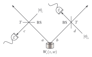
Figure 9: Scheme of the IPS process.

First of all we briefly recall the IPS process, whose scheme is sketched in Fig. 9. The two modes, $a$ and $b$, of the TWB are mixed with the vacuum (modes $c$ and $d$, respectively) at two unbalanced beam splitters (BS) with equal transmissivity; the modes $c$ and $d$ are then detected by avalanche photodetectors (APDs) with equal efficiency, which can only discriminate the presence of radiation from the vacuum: the IPS state is obtained when the two detectors jointly click. When the input state, namely the state arriving at the two beam splitters, is the TWB of Eq. (31), the state produced by the IPS process reads as follows (see Ref. ips:PRA:70 for details)

$$W_{r,T,\varepsilon}^{\rm(IPS)}(z,w)=\frac{4}{\pi^{2}\,p_{11}(r,T,\varepsilon)}\sum_{k=1}^{4}{\cal C}_{k}\,W_{r,T,\varepsilon}^{(k)}(z,w)\,,$$ (42)

where

$$p_{11}(r,T,\varepsilon)=\sum_{k=1}^{4}\frac{{\cal C}_{k}}{F_{k}G_{k}-H_{k}^{2}}\,$$ (43)

is the probability of a click in both the APDs. In Eqs. (42) and (43) we introduced

$${\cal C}_{k}\equiv{\cal C}_{k}(r,T,\varepsilon)=\frac{4\,C_{k}}{x_{k}y_{k}-4B^{2}(1-T)^{2}}\,,$$ (44)

and defined

$$W_{r,T,\varepsilon}^{(k)}(z,w)=\exp\{- F_{k}|z|^{2}-G_{k}|w|^{2}$$

$$+H_{k}(zw+z^{*}w^{*})\}\,,$$ (45)

where $F_{k}=(b-f_{k})$, $G_{k}=(b-g_{k})$, $H_{k}=(2BT+h_{k})$, $C_{k}\equiv C_{k}(\varepsilon)$ with $C_{1}=1$, $C_{2}=C_{3}=-2(2-\varepsilon)^{-1}$, $C_{4}=4(2-\varepsilon)^{-2}$; $x_{k}\equiv x_{k}(r,T,\varepsilon)$ and $y_{k}\equiv y_{k}(r,T,\varepsilon)$ are

$$x_{1}=x_{3}=y_{1}=y_{2}=a$$

$$x_{2}=x_{4}=y_{3}=y_{4}=a+2\varepsilon(2-\varepsilon)^{-1}$$

with $a\equiv a(r,T)=2[A(1-T)+T]$, $b\equiv b(r,T)=2[AT+(1-T)]$; finally, $f_{k}$, $g_{k}$, and $h_{k}$ depend on $r$, $T$ and $\varepsilon$ and are given by

$$f_{k} ={\cal N}_{k}\,[x_{k}B^{2}$$

$$\hskip 42.67912pt+4B^{2}(1-A)(1-T)+y_{k}(1-A)^{2}]\,,$$ (46)

$$g_{k} ={\cal N}_{k}\,[x_{k}(1-A)^{2}$$

$$\hskip 42.67912pt+4B^{2}(1-A)(1-T)+y_{k}B^{2}]\,,$$ (47)

$$h_{k} ={\cal N}_{k}\,\{(x_{k}+y_{k})B(1-A)$$

$$\hskip 42.67912pt+2B[B^{2}+(1-A)^{2}](1-T)\}\,,$$ (48)

$${\cal N}_{k} \equiv{{\cal N}_{k}}(r,T,\varepsilon)={\displaystyle\frac{4T\,(1-T)}{x_{k}y_{k}-4B^{2}(1-T)^{2}}\,.}$$ (49)

The state given in Eq. (42) is no longer a Gaussian state and, in the following, we will use the measurement described above in order to test its nonlocality. Nonlocal properties of the IPS state (42) have been investigated in Refs. ips:PRA:70 ; ips:noise by means of other kinds of nonlocality tests. In particular, Ref. ips:noise addressed the presence of noise during the propagation and detection stages, showing that the IPS process onto TWBs is a quite robust method to enhance their nonlocal correlations especially in the low energy (i.e., small $r$) regime.

In the case of the state (42), the correlation function (3) reads (for the sake of simplicity we do not write explicitly the dependence on $r$, $T$ and $\varepsilon$)

$$E_{\eta}(\alpha,\beta)= \frac{1}{p_{11}(r,T,\varepsilon)}\sum_{k=1}^{4}{\cal C}_{k}\,\big{\{}1+4\,{\cal I}^{(k)}_{\eta}(\alpha,\beta)$$

$$-2\big{[}{\cal G}^{(k)}_{\eta}(\alpha)+{\cal Y}^{(k)}_{\eta}(\beta)\big{]}\big{\}}\,,$$ (50)

where

$${\cal I}^{(k)}_{\eta}(\alpha,\beta)= \frac{4{\cal M}_{\eta}^{(k)}(r,T,\varepsilon)}{\eta^{2}}\,\exp\big{\{}-\widetilde{G}_{\eta}^{(k)}\,|\alpha|^{2}$$

$$-\widetilde{F}_{\eta}^{(k)}\,|\beta|^{2}+\widetilde{H}_{\eta}^{(k)}\,(\alpha\beta+\alpha^{*}\beta^{*})\big{\}}\,,$$ (51)

with $\widetilde{F}_{\eta}^{(k)}\equiv\widetilde{F}_{\eta}^{(k)}(r,T,\varepsilon)$, $\widetilde{G}_{\eta}^{(k)}\equiv\widetilde{G}_{\eta}^{(k)}(r,T,\varepsilon)$, and $\widetilde{H}_{\eta}^{(k)}\equiv\widetilde{H}_{\eta}^{(k)}(r,T,\varepsilon)$ given by

$$\widetilde{F}_{\eta}^{(k)}=\Delta_{\eta}-(F_{k}+\Delta_{\eta})\,{\cal M}_{\eta}^{(k)}(r,T,\varepsilon)\,,$$ (52)

$$\widetilde{G}_{\eta}^{(k)}=\Delta_{\eta}-(G_{k}+\Delta_{\eta})\,{\cal M}_{\eta}^{(k)}(r,T,\varepsilon)\,,$$ (53)

$$\widetilde{H}_{\eta}^{(k)}=H_{k}\,{\cal M}_{\eta}^{(k)}(r,T,\varepsilon)\,,$$ (54)

$${\cal M}_{\eta}^{(k)}(r,T,\varepsilon)=\frac{\Delta_{\eta}^{2}}{(F_{k}+\Delta_{\eta})(G_{k}+\Delta_{\eta})-H_{k}^{2}}\,,$$ (55)

respectively, and

$${\cal G}^{(k)}_{\eta}(\alpha)= \frac{4\Delta_{\eta}}{[G_{k}\,(F_{k}+\Delta_{\eta})-H_{k}^{2}]\,\eta}$$

$$\times\exp\left\{-\frac{(F_{k}G_{k}-H_{k}^{2})\,\Delta_{\eta}}{G_{k}\,(F_{k}+\Delta_{\eta})-H_{k}^{2}}\,|\alpha|^{2}\right\}\,,$$ (56)

$${\cal Y}^{(k)}_{\eta}(\beta)= \frac{4\Delta_{\eta}}{[F_{k}\,(G_{k}+\Delta_{\eta})-H_{k}^{2}]\,\eta}$$

$$\times\exp\left\{-\frac{(F_{k}G_{k}-H_{k}^{2})\,\Delta_{\eta}}{F_{k}\,(G_{k}+\Delta_{\eta})-H_{k}^{2}}\,|\beta|^{2}\right\}\,.$$ (57)

In order to investigate the nonlocality of the IPS by means of Eq. (6), we choose the same parametrization as in Sec. V. The results are showed in Figs. 10 and 11 for $\eta=1$ and $\varepsilon=1$: we can see that the IPS enhances the violation of the inequality $|{\cal B}_{\eta}|\leq 2$ for small values of $r$ (see also Refs. ips:PRA:67 ; ips:PRA:70 ; ips:noise ). Moreover, as one may expect, the maximum of violation is achieved as $T\to 1$, whereas decreasing the effective transmission of the IPS process, one has that the inequality becomes satisfied for all the values of $r$, as we can see in Fig. 11 for $\tau=0.8$.

In Fig. 12 we plot ${\cal B}_{\eta}$ for the IPS with $T=0.9999$, $\varepsilon=1$ and different $\eta$. As for the TWB, we can have violation of the Bell’s inequality also for detection efficiencies near to $80\%$. As for the Bell states and the TWB, a $\eta$- and $r$-dependent choice of the parameters in Eq. (6) can improve this result. The effect on a non-unit $\varepsilon$ is studied in Fig. 13, where we plot ${\cal B}_{\eta}$ as a function of $T$ and $\varepsilon$ and fixed values of the other involved parameters. We can see that the main effect on the Bell parameter is due to the transmissivity $T$.

The presence of dark counts at the detection stage can be taken into account using Eqs. (7): since the results are similar to those of the Bells states and the TWB presented in Sec. VI, we do not report them explicitly.

VIII Choice of the parametrization

In this Section we draw some remark about the choice of the parametrization used in the investigation of the Bell parameter ${\cal B}_{\eta}$. Numerical analysis has shown that, in the case of state $|\Psi_{+}\rangle$ and in the presence of non-unit quantum efficiency, the maximal violation of the Bell’s inequality for the displaced on/off test is achieved by choosing $\alpha$, $\alpha^{\prime}$, $\beta$, and $\beta^{\prime}$ as complex parameters bana:pra:02 . On the other hand, here we addressed only real parametrization for the Bell’s parameter ${\cal B}$ given in Eq. (6), and, in particular, we take $\alpha=-\beta={\cal J}\in\mathbb{R}$, and $\alpha^{\prime}=-\beta^{\prime}={\cal J}^{\prime}\in\mathbb{R}$ for the states $|\Psi_{+}\rangle$, $|\Phi_{+}\rangle$, the TWB and the IPS state, while we put $\alpha=\beta={\cal J}\in\mathbb{R}$ and $\alpha^{\prime}=\beta^{\prime}={\cal J}^{\prime}\in\mathbb{R}$ for the states $|\Psi_{-}\rangle$ and $|\Phi_{-}\rangle$. In Fig. 14 we plot $|{\cal B}_{\eta}|$ as a function of ${\cal J}$ and ${\cal J}^{\prime}$ in the ideal case (i.e., $\eta=1$) for (a) the states $|\Psi_{\pm}\rangle$ and (b) the TWB with $r=0.74$, which maximizes the violation. The results for the other states are similar. In both the plots, the darker is the region, the bigger is the violation (the white region refers to $|{\cal B}_{\eta}|\leq 2$). As one can see, there is a symmetry with respect to the origin, which implies that the best parametrization has the form ${\cal J}^{\prime}=-\kappa{\cal J}$, with $\kappa\in\mathbb{R}$, $\kappa>0$. Furthermore, for all the considered states, the numerical analysis shows that a good choice for $\kappa$ is $\kappa=\sqrt{11}$, which is an approximation of the actual value.

In Fig. 15 the effect of $\eta$ is taken into account: Since the results for the Bell’s states, the TWB and the IPS state are similar, we only address the TWB case: there is still the symmetry with respect to the origin, but a thorough numerical investigation shows that the maximum of ${\cal B}_{\eta}$, and, then, $\kappa$ depend on both $\eta$ and $r$.

Notice that we have considered real values for the parameters. It can be shown numerically bana:pra:02 that for decreasing $\eta$ a complex parametrization leads to a slight improvement.

IX Bell’s inequality, POVMs and maximum violation

In this Section we address the maximal violation of the Bell inequality that is achievable by using non-projective measurements.

Let us consider two systems, ${\sf A}$ and ${\sf B}$, and the generic POVM $\{\Pi_{0}(\zeta),\Pi_{1}(\zeta)\}$, depending on the complex parameter $\zeta$, such that $\Pi_{1}(\zeta)=\mathbb{I}-\Pi_{0}(\zeta)$. We define the observables

$${\mathscr{O}}_{\sf k}(\zeta)=\Pi_{1}(\zeta)-\Pi_{0}(\zeta)=\mathbb{I}-2\,\Pi_{0}(\zeta)$$ (58)

acting on system ${\sf k}={\sf A},{\sf B}$, respectively (we are using the same POVM for both the systems). Furthermore, we assume that ${\mathscr{O}}_{\sf A}(\zeta)$ and ${\mathscr{O}}_{\sf B}(\zeta)$ have spectra included in the interval $[-1,+1]$ cirelsonB . Now we introduce the Bell operator CHSH

$${\mathscr{B}}= {\mathscr{O}}_{\sf A}(\alpha)\otimes{\mathscr{O}}_{\sf B}(\beta)+{\mathscr{O}}_{\sf A}(\alpha^{\prime})\otimes{\mathscr{O}}_{\sf B}(\beta)$$

$$+{\mathscr{O}}_{\sf A}(\alpha)\otimes{\mathscr{O}}_{\sf B}(\beta^{\prime})-{\mathscr{O}}_{\sf A}(\alpha^{\prime})\otimes{\mathscr{O}}_{\sf B}(\beta^{\prime})\,,$$ (59)

which has the property cirelsonB

$${\mathscr{B}}\leq\frac{1}{\sqrt{2}}\big{[} {\mathscr{O}}_{\sf A}^{2}(\alpha)\otimes\mathbb{I}+\mathbb{I}\otimes{\mathscr{O}}_{\sf B}^{2}(\beta)$$

$$+{\mathscr{O}}_{\sf A}^{2}(\alpha^{\prime})\otimes\mathbb{I}+\mathbb{I}\otimes{\mathscr{O}}_{\sf B}^{2}(\beta^{\prime})\big{]}\,.$$ (60)

If $\Pi_{1}(\zeta)$ and $\Pi_{0}(\zeta)$ are projectors on orthogonal subspaces, namely $\Pi_{1}^{2}(\zeta)=\Pi_{1}(\zeta)$, $\Pi_{0}^{2}(\zeta)=\Pi_{0}(\zeta)$ and $\Pi_{0}(\zeta)\,\Pi_{1}(\zeta)=0$, then

$${\mathscr{O}}_{\sf A}^{2}(\zeta)={\mathscr{O}}_{\sf B}^{2}(\xi)=\mathbb{I}\,,$$ (61)

and Eq. (60) leads to

$${\cal B}\leq 2\sqrt{2}\,,$$ (62)

where ${\cal B}={\rm Tr}[\varrho\,{\mathscr{B}}]$, $\varrho$ being the state of the system, is the Bell parameter. The bound $2\sqrt{2}$ is usually known as Cirel’son bound and is the maximum violation achievable in the case of a bipartite quantum system cirelsonB . Eq. (62) may be also derived in a different landau ; peres : since the squared Bell operator reads

$${\mathscr{B}}^{2}=4\mathbb{I}+\left[{\mathscr{O}}_{\sf A}(\alpha),{\mathscr{O}}_{\sf A}(\alpha^{\prime})\right]\otimes\left[{\mathscr{O}}_{\sf B}(\beta),{\mathscr{O}}_{\sf B}(\beta^{\prime})\right]\,,$$ (63)

then using the relation $||[A,B]||\leq 2||A||\,||B||$, where $||A||={\rm Sup}_{|\psi\rangle}||A|\psi\rangle||$, we have ${\cal B}^{2}\leq 8$, from which Eq. (62) follows.

On the other hand, when $\{\Pi_{0}(\zeta),\Pi_{1}(\zeta)\}$ is not a projective measurement a different inequality should be derived. First of all we note that the observables ${\mathscr{O}}_{\sf k}(\zeta)$ corresponding to the POVM given in Eq. (1) satisfy the hypothesis of the Cirel’son theorem. In fact, in this case

$${\mathscr{O}}_{\sf k}(\zeta)=\sum_{n=0}^{\infty}\left[1-2(1-\eta)^{n}\right]D(\zeta)|n\rangle\langle n|D^{{\dagger}}(\zeta)$$ (64)

and its spectrum $\{\lambda_{n}\}$, $\lambda_{n}=1-2(1-\eta)^{n}$, lies in the interval $[-1,+1]$ for $0\leq\eta\leq 1$ (when $\eta=1$ the spectrum reduces to the two points $\{-1,+1\}$). Now, one has

$${\mathscr{O}}_{\sf A}^{2}(\zeta) =\mathbb{I}-4\,\Pi_{0}(\zeta)\,\Pi_{1}(\zeta)=\mathbb{I}-4\,[\Pi_{0}(\zeta)-\Pi_{0}^{2}(\zeta)]$$

$$=\mathbb{I}-4\,{\mathscr{E}}_{\sf A}(\zeta)\,,$$ (65)

and, analogously, ${\mathscr{O}}_{\sf B}^{2}(\xi)=\mathbb{I}-4\,{\mathscr{E}}_{\sf B}(\xi)$, where we defined the operator

$${\mathscr{E}}_{\sf k}(\zeta)=\Pi_{0}(\zeta)-\Pi_{0}^{2}(\zeta)\,,$$ (66)

${\sf k}={\sf A},{\sf B}$. In this way, from Eq. (60) follows

$${\mathscr{B}}\leq 2\sqrt{2}\big{\{}\mathbb{I}-[{\mathscr{E}}_{\sf A}(\alpha)+{\mathscr{E}}_{\sf B}(\beta)+{\mathscr{E}}_{\sf A}(\alpha^{\prime})+{\mathscr{E}}_{\sf B}(\beta^{\prime})]\big{\}}\,,$$ (67)

with ${\mathscr{E}}_{\sf A}(\zeta)\equiv{\mathscr{E}}_{\sf A}(\zeta)\otimes\mathbb{I}$ and ${\mathscr{E}}_{\sf B}(\xi)\equiv\mathbb{I}\otimes{\mathscr{E}}_{\sf B}(\xi)$. Finally we get

$${\cal B}\leq{\cal B}^{\rm(max)}(\alpha,\beta,\alpha^{\prime},\beta^{\prime})\,,$$ (68)

where we defined

$${\cal B}^{\rm(max)} \equiv{\cal B}^{\rm(max)}(\alpha,\beta,\alpha^{\prime},\beta^{\prime})$$ (69)

$$=2\sqrt{2}\big{\{}1-[{\cal E}_{\sf A}(\alpha)+{\cal E}_{\sf B}(\beta)$$

$$\hskip 85.35826pt+{\cal E}_{\sf A}(\alpha^{\prime})+{\cal E}_{\sf B}(\beta^{\prime})]\big{\}}$$ (70)

and ${\cal E}_{\sf A}(\zeta)={\rm Tr}[{\mathscr{E}}_{\sf A}(\zeta)\otimes\mathbb{I}]$ and ${\cal E}_{\sf B}(\xi)={\rm Tr}[\mathbb{I}\otimes{\mathscr{E}}_{\sf B}(\xi)]$. Now, since ${\cal E}_{\sf k}\geq 0$, ${\sf k}={\sf A},{\sf B}$, one has that the bound of the Bell parameter is smaller than the limit $2\sqrt{2}$, obtained in the case of projective measurements. Notice that the new bound depends on the parameters $\alpha$, $\beta$, $\alpha^{\prime}$, and $\beta^{\prime}$ of the measurement and on the state under investigation itself.

In the following we address the problem of evaluating the maximum violation for the Bell states, the TWB and the IPS state when a non-unit efficiency affects the displaced on/off photodetection. First of all we note that

$$\Pi_{0,\eta}^{2}=\sum_{k=0}^{\infty}(1-\eta)^{2k}|k\rangle\langle k|=\Pi_{0,\eta(2-\eta)}\,,$$ (71)

so that

$${\cal E}_{\sf A}(\zeta) ={\cal G}_{\eta}(\zeta)-{\cal G}_{\eta(2-\eta)}(\zeta)$$ (72)

$${\cal E}_{\sf B}(\xi) ={\cal Y}_{\eta}(\zeta)-{\cal Y}_{\eta(2-\eta)}(\xi)\,.$$ (73)

In this way it is straightforward to evaluate ${\cal B}^{\rm(max)}_{\eta}$ for the Bell states, the TWB and the IPS state. The results are shown in the Figs. 16–21: in Figs. 17, 19, and 21 we plot ${\cal B}^{\rm(max)}_{\eta}$ using the parametrization $\alpha=\beta={\cal J}$ and $\alpha^{\prime}=\beta^{\prime}=\sqrt{11}\,{\cal J}$, which maximizes the Bell parameter ${\cal B}_{\eta}$. It is worth noticing that for all the considered states and for fixed ${\cal J}$ the limit ${\cal B}^{\rm(max)}_{\eta}$ is never reached; on the other hand, even if the actual maximum violation, i.e., ${\cal B}_{\eta,{\rm max}}$, is quite lower than the Cirel’son bound $2\sqrt{2}$, it is relatively near to the new bound given by Eq. (68).

Notice that a similar analysis may be performed through the squared Bell operator, which for ${\mathscr{O}}_{\sf k}^{2}(\zeta)\neq\mathbb{I}$ is given by

$${\mathscr{B}}^{2}=\left({\mathscr{O}}_{\sf A}^{2}(\alpha)+{\mathscr{O}}_{\sf A}^{2}(\alpha^{\prime})\right)\otimes\left({\mathscr{O}}_{\sf B}^{2}(\beta)+{\mathscr{O}}_{\sf B}^{2}(\beta^{\prime})\right)\\ +\left({\mathscr{O}}_{\sf A}^{2}(\alpha)-{\mathscr{O}}_{\sf A}^{2}(\alpha^{\prime})\right)\otimes\left[{\mathscr{O}}_{\sf B}(\beta),{\mathscr{O}}_{\sf B}(\beta^{\prime})\right]_{+}\\ -\left[{\mathscr{O}}_{\sf A}(\alpha),{\mathscr{O}}_{\sf A}(\alpha^{\prime})\right]_{+}\otimes\left({\mathscr{O}}_{\sf B}^{2}(\beta)-{\mathscr{O}}_{\sf B}^{2}(\beta^{\prime})\right)\\ +\left[{\mathscr{O}}_{\sf A}(\alpha),{\mathscr{O}}_{\sf A}(\alpha^{\prime})\right]\otimes\left[{\mathscr{O}}_{\sf B}(\beta)+{\mathscr{O}}_{\sf B}(\beta^{\prime})\right]\,,$$ (74)

$[A,B]_{+}=AB+BA$ being the anti-commutator. As for Eq. (68), the maximum value of Eq. (74) depends on the state under investigation and on the POVM itself.

X Concluding remarks

We have analyzed in details the nonlocality of several two-mode (entangled) states of light by using a test based on displaced on/off photodetection. Nonlocality has been quantified through violation of CHSH inequality for the Bell’s parameter. Effects due to non-unit quantum efficiency and nonzero dark counts have been taken into account. We found that unbalanced superpositions show larger nonlocality than balanced one when noise affects the photodetection process, and that twin-beam nonlocality is more robust than that of superpositions of few photon-number states. De-Gaussification by means of (inconclusive) photon subtraction is shown to enhance nonlocality of twin beams in the low energy regime. We have also shown that, since our measurement is described by a POVM rather than a set of projectors, the maximum violation the CHSH inequality cannot saturate the Cirel’son bound. A novel state-dependent bound has been derived.

Appendix A Noisy on/off photodetection

The action of an on/off detector in the ideal case is described by the two-value POVM $\{\Pi_{0}=|0\rangle\langle 0|,\Pi_{1}={\mathbb{I}}-\Pi_{0}\}$, which represents a partition of the Hilbert space of the signal. In the realistic case the performances of on/off photodetectors are degraded by two effects. On one hand, one has non-unit quantum efficiency, i.e., the loss of a portions of the incoming photons, and, on the other hand, there is also the presence of dark-count, i.e., by "clicks" that do not correspond to any incoming photon. In order to take into account both these effects we use a simple scheme described in the following.

A real photodetector is modeled as an ideal photodetector (unit quantum efficiency, no dark-count) preceded by a beam splitter (of transmissivity equal to the quantum efficiency $\eta$) whose second port is in an auxiliary excited state $\nu$, which can be a thermal state, or a phase-averaged coherent state, depending on the kind of background noise (thermal or Poissonian). If the second port of the beam splitter is the vacuum $\nu=|0\rangle\langle 0|$ we have no dark-count; for the second port of the BS excited in a generic mixture $\nu=\sum_{s}\nu_{ss}|s\rangle\langle s|$ the POVM for the on/off photodetection is given by ($\Pi_{1}={\mathbb{I}}-\Pi_{0}$)

$$\Pi_{0}=\sum_{n=0}^{\infty}(1-\eta)^{n}\sum_{s=0}^{\infty}\nu_{ss}\>\eta^{s}\>\binom{n+s}{s}\>|n\rangle\langle n|\;.$$ (75)

The density matrices of a thermal state and a phase-averaged coherent state (with $M$ mean photons) are given by

$$\nu_{\hbox{\tiny T}} = \frac{1}{M+1}\sum_{s}\left(\frac{M}{M+1}\right)^{s}\>|s\rangle\langle s|$$ (76)

$$\nu_{\hbox{\tiny P}} = e^{-M}\sum_{s}\frac{M^{s}}{s!}|s\rangle\langle s|\;.$$ (77)

In order to reproduce a background noise with mean photon number $D$ we consider the state $\nu$ with average photon number $M=D/(1-\eta)$. In this case we have

$$\Pi_{0,\eta,D}^{\hbox{\tiny T}} = \frac{1}{1+D}\sum_{n}\left(1-\frac{\eta}{1+D}\right)^{n}\>|n\rangle\langle n|$$ (78)

$$\Pi_{0,\eta,D}^{\hbox{\tiny P}} = e^{-D}\sum_{n}\Bigg{[}(1-\eta)^{n}\>L_{n}\left(-D\frac{\eta}{1-\eta}\right)\Bigg{]}\>|n\rangle\langle n|\;,$$ (79)

where T and P denotes thermal and Poissonian respectively, and $L_{n}(x)$ is the Laguerre polynomial of order $n$. The corresponding Wigner functions are given by

$$W[\Pi^{\hbox{\tiny T}}_{0,\eta,D}](\alpha) = \frac{1}{\pi}\frac{2}{2(1+D)-\eta}\exp\left\{-\frac{2\eta}{2(1+D)-\eta}\,|\alpha|^{2}\right\}\,,$$ (80)

$$W[\Pi^{\hbox{\tiny P}}_{0,\eta,D}](\alpha) = \frac{1}{\pi}\>\frac{2}{2-\eta}\exp\left\{-\frac{2\eta}{2-\eta}(D+|\alpha|^{2})\right\}\>I_{0}\left(\frac{4|\alpha|\sqrt{\eta D}}{2-\eta}\right)\;,$$ (81)

respectively, where $I_{0}(x)$ is the $0$-th modified Bessel function of the first kind. For small $D$ the POVMs coincide up to first order, as well as the corresponding Wigner functions.

Figure 2: Plot of $-{\cal B}_{\eta}$ for the states $|\Psi_{\pm}\rangle$ (a) and of ${\cal B}_{\eta}$ for $|\Phi_{\pm}\rangle$ (b) as functions of ${\cal J}$ and $\eta$. The maximum violations for $\eta=1$ are: (a) $-{\cal B}_{\eta}=2.69$, and (b) ${\cal B}_{\eta}=2.68$, which are both obtained when ${\cal J}=0.17$. For the particular choice of the parametrizations ${\cal B}_{\eta}$ is the same for $|\Psi_{\pm}\rangle$ and for $|\Phi_{\pm}\rangle$.

Figure 3: Plot of $-{\cal B}_{\eta}$: (a) for $|\Psi_{\varphi}\rangle$ as a function of ${\cal J}$ and $\varphi$ in the case of ideal (i.e., $\eta=1$) on/off photodetection; (b) for ${\cal J}=0.17$ and different values of $\eta$: from bottom to top $\eta=1.0$, $0.9$, $0.85$, and $0.8$. The vertical line is $\varphi=\pi/4$.

Figure 4: Plot of ${\cal B}_{\eta}$: (a) for $|\Phi_{\varphi}\rangle$ as a function of ${\cal J}$ and $\varphi$ in the case of ideal (i.e., $\eta=1$) on/off photodetection; (b) for ${\cal J}=0.17$ and different values of $\eta$: from top to bottom $\eta=1.0$, $0.9$, $0.85$, $0.8$, and $0.75$. The vertical line is $\varphi=\pi/4$.

Figure 5: Plot of $-{\cal B}_{\eta}$ for the superposition of two photons as a function of ${\cal J}$ and $\eta$. The maximum violation is $-{\cal B}_{\eta}=2.07$, which is obtained when ${\cal J}=0.45$ and $\eta=1$.

Figure 6: Plot of ${\cal B}_{\eta}$ for a TWB as a function of ${\cal J}$ and the TWB squeezing parameter $r$ in the case of ideal (i.e., $\eta=1$) on/off photodetection. The maximum violation is ${\cal B}_{\eta}=2.45$, which is obtained when ${\cal J}=0.16$ and $r=0.74$.

Figure 7: Plot of ${\cal B}_{\eta}$ for a TWB as a function of ${\cal J}$ with $r=0.74$ for different values of $\eta$: from top to bottom $\eta=1.0$, $0.9$, $0.85$, and $0.80$.

Figure 8: Plot of ${\cal B}_{\eta,D}(\alpha,\beta,\alpha^{\prime},\beta^{\prime})$ for the Bell states $|\Phi_{\pm}\rangle$ (upper plot) and the TWB (lower plot). We set ${\cal J}=0.17$ for the Bell states, ${\cal J}=0.16$ and $r=0.74$ for the TWB, and used the parametrizations introduced in Secs. III and V, respectively.

Figure 10: Plot of ${\cal B}_{\eta}$ for the IPS state with $T=0.9999$ and $\varepsilon=1$ as a function of ${\cal J}$ and the TWB squeezing parameter $r$ in the case of ideal (i.e., $\eta=1$) on/off photodetection. The maximum violation is ${\cal B}_{\eta}=2.53$, which is obtained when ${\cal J}=0.16$ and $r=0.39$.

Figure 11: Plot of ${\cal B}_{\eta}$ for the IPS state as a function of ${\cal J}$ with $r=0.39$ for different values of $T$ and $\varepsilon=1$ in the ideal case (i.e., $\eta=1$): from top to bottom $T=0.9999$, $0.95$, $0.90$, and $0.80$.

Figure 12: Plot of ${\cal B}_{\eta}$ for the IPS state as a function of ${\cal J}$ with $r=0.39$, $T=0.9999$, $\varepsilon=1$, and for different values of $\eta$: from top to bottom $\eta=1.0$, $0.9$, $0.85$, and $0.8$.

Figure 13: Plot of ${\cal B}_{\eta}$ for the IPS state as a function $T$ and $\varepsilon$ with ${\cal J}=0.16$, $r=0.39$, and, from top to bottom, $\eta=0.99$, and $0.90$. The main effect on ${\cal B}_{\eta}$ is due to the transmissivity $T$.

Figure 14: Plots of $|{\cal B}_{\eta}|$ for (a) the states $|\Psi_{\pm}\rangle$ and (b) the TWB with $r=0.74$ and $\eta=1$. The darker is the region, the bigger is the violation of the Bell’s inequality. In the white region $|{\cal B}_{\eta}|\leq 2$. ${\cal J}$ and ${\cal J}^{\prime}$ refer to the particular parametrization of ${\cal B}_{\eta}$, see the text for details.

Figure 15: Plots of ${\cal B}_{\eta}$ in the case of TWB for different $\eta$. The TWB parameter $r$ is chosen in order to maximize the violation of the Bell’s inequality as $\eta$ varies. We put (a) $\eta=1$, $r=0.74$ (${\cal B}_{\eta,{\rm max}}=2.45$), (b) $\eta=0.9$, $r=0.67$ (${\cal B}_{\eta,{\rm max}}=2.24$), (c) $\eta=0.85$, $r=0.60$ (${\cal B}_{\eta,{\rm max}}=2.15$), and (d) $\eta=0.8$, $r=0.49$ (${\cal B}_{\eta,{\rm max}}=2.07$). ${\cal J}$ and ${\cal J}^{\prime}$ refer to the particular parametrization of ${\cal B}_{\eta}$, see the text for details. Since there is symmetry with respect to the origin, we show only the region ${\cal J}^{\prime}\geq 0$.

Figure 16: Plot of ${\cal B}^{\rm(max)}_{\eta}(\alpha,\beta,\alpha^{\prime},\beta^{\prime})$ for the Bell states. We set $\alpha=\beta={\cal J}$ and $\alpha^{\prime}=\beta^{\prime}={\cal J^{\prime}}$ and: (a) $\eta=0.9$, (b) $\eta=0.8$.

Figure 17: Plots of ${\cal B}^{\rm(max)}_{\eta}(\alpha,\beta,\alpha^{\prime},\beta^{\prime})$ in the case of the Bell states for different values of $\eta$; from top to bottom (solid lines): $\eta=0.95,0.9,0.85$, and $0.8$. The dashed line corresponds to the value $2\sqrt{2}$ obtained when $\eta=1$. We set $\alpha=\beta={\cal J}$ and $\alpha^{\prime}=\beta^{\prime}=\sqrt{11}\,{\cal J}$, which maximize ${\cal B}$.

Figure 18: Plot of ${\cal B}^{\rm(max)}_{\eta}(\alpha,\beta,\alpha^{\prime},\beta^{\prime})$ for the TWB with $r=0.74$. We set $\alpha=\beta={\cal J}$ and $\alpha^{\prime}=\beta^{\prime}={\cal J^{\prime}}$ and: (a) $\eta=0.9$, (b) $\eta=0.8$.

Figure 19: Plots of ${\cal B}^{\rm(max)}_{\eta}(\alpha,\beta,\alpha^{\prime},\beta^{\prime})$ in the case of the TWB with $r=0.74$ for different values of $\eta$; from top to bottom (solid lines): $\eta=0.95,0.9,0.85$, and $0.8$. The dashed line corresponds to the value $2\sqrt{2}$ obtained when $\eta=1$. We set $\alpha=\beta={\cal J}$ and $\alpha^{\prime}=\beta^{\prime}=\sqrt{11}\,{\cal J}$, which maximize ${\cal B}$.

Figure 20: Plot of ${\cal B}^{\rm(max)}_{\eta}(\alpha,\beta,\alpha^{\prime},\beta^{\prime})$ for the IPS state with $r=0.39$, $T=0.9999$, and $\varepsilon=1$. We set $\alpha=\beta={\cal J}$ and $\alpha^{\prime}=\beta^{\prime}={\cal J^{\prime}}$ and: (a) $\eta=0.9$, (b) $\eta=0.8$.

Figure 21: Plots of ${\cal B}^{\rm(max)}_{\eta}(\alpha,\beta,\alpha^{\prime},\beta^{\prime})$ in the case of the IPS state with $r=0.39$, $T=0.9999$, and $\varepsilon=1$ for different values of $\eta$; from top to bottom (solid lines): $\eta=0.95,0.9,0.85$, and $0.8$. The dashed line corresponds to the value $2\sqrt{2}$ obtained when $\eta=1$. We set $\alpha=\beta={\cal J}$ and $\alpha^{\prime}=\beta^{\prime}=\sqrt{11}\,{\cal J}$, which maximize ${\cal B}$.

References

• (1) R. F. Werner, Phys. Rev. A 40, 4277 (1989).
• (2) K. Banaszek, and K. Wódkiewicz, Phys. Rev. Lett. 82, 2009 (1999).
• (3) A. Ferraro, S. Olivares, and M. G. A. Paris, Gaussian States in Quantum Information (Bibliopolis, Napoli, 2005).
• (4) J. F. Clauser, M. A. Horne, A. Shimony, and R. A. Holt, Phys. Rev. Lett. 23, 880 (1969).
• (5) J. F. Clauser, M. A. Horne, Phys. Rev. D 10, 526 (1974)
• (6) K. Banaszek, A. Dragan, K. Wódkiewicz, and C. Radzewicz Phys. Rev. A 66, 043803 (2002).
• (7) S. Olivares, M. G. A. Paris, and R. Bonifacio, Phys. Rev. A 67,032314 (2003).
• (8) T. Opatrný, G. Kurizki, and D.-G. Welsch, Phys. Rev. A 61, 032302 (2000).
• (9) P. T. Cochrane, T. C. Ralph, and G. J. Milburn, Phys. Rev. A 65, 062306 (2002).
• (10) H. Nha, and H. J. Carmichael, Phys. Rev. Lett. 93, 020401 (2004).
• (11) R. García-Patrón Sánchez et al., Phys. Rev. Lett. 93, 130409 (2004).
• (12) S. Olivares, and M. G. A. Paris, Phys. Rev. A 70, 032112 (2004).
• (13) S. Olivares, and M. G. A. Paris, quant-ph/0503104.
• (14) B. S. Cirel’son, Lett. Math. Phys. 4, 93 (1980).
• (15) L. J. Landau, Phys. Lett A 120, 54 (1987).
• (16) A. Peres, Quantum Theory: Concepts and Methods (Kluwer, Dordrecht, 1993).
Refer to caption