Lorentz–covariant reduced spin density matrix and Einstein–Podolsky–Rosen–Bohm correlations

Abstract

We show that it is possible to define a Lorentz–covariant reduced spin density matrix for massive particles. Such a matrix allows one to calculate the mean values of observables connected with spin measurements (average polarizations). Moreover, it contains not only information about polarization of the particle but also information about its average kinematical state. We also use our formalism to calculate the correlation function in the Einstein–Podolsky–Rosen–Bohm type experiment with massive relativistic particles.

I Introduction

Relativistic aspects of quantum mechanics have recently attracted much attention, especially in the context of the theory of quantum information. One of the important questions in this context is how to define the reduced spin density matrix. Such a matrix should enable one to make statistical predictions for the outcomes of ideal spin measurements which are not influenced by the particle momentum. We consider this problem in detail in the case of massive particles. The reduced spin density matrix is usually defined by the following formula Peres et al. (2002):

$$\tau_{\sigma\lambda}=\int d\mu(k)\left<k,m,s,\sigma\right|\hat{\rho}\left|k,m,s\lambda\right>,$$ (1)

where $\hat{\rho}$ denotes the complete density matrix of a single particle with mass $m$, $d\mu(k)=\frac{d^{3}k}{2k^{0}}$ is the Lorentz–invariant measure on the mass shell and four-momentum eigenvectors $\left|k,m,s,\lambda\right>$ (i.e., $P_{\mu}\left|k,m,s,\lambda\right>=k_{\mu}\left|k,m,s,\lambda\right>$) span the space of the irreducible representation of the Poincaré group. They are normalized as follows

$$\left<p,m,s,\sigma|k,m,s,\lambda\right>=2k^{0}\delta^{3}(\mathbf{k}-\mathbf{p})\delta_{\sigma\lambda}.$$ (2)

The action of the Lorentz transformation $\Lambda$ on the vector $\left|k,m,s,\lambda\right>$ is of the form

$$U(\Lambda)\left|k,m,s,\lambda\right>={\mathcal{D}}_{\sigma\lambda}^{s}(R(\Lambda,k))\left|\Lambda k,m,s,\sigma\right>,$$ (3)

where ${\mathcal{D}}^{s}$ is the matrix spin $s$ representation of the $SO(3)$ group, $R(\Lambda,k)=L_{\Lambda k}^{-1}\Lambda L_{k}$ is the Wigner rotation and $L_{k}$ designates the standard Lorentz boost defined by the relations $L_{k}\tilde{k}=k$, $L_{\tilde{k}}=I$, $\tilde{k}=(m,\mathbf{0})$.

The key question is whether the reduced density matrix is covariant. In Peres et al. (2002) it was stressed that the matrix (1) is not covariant under Lorentz boosts. It means that when we calculate the complete density matrix as seen by the boosted observer

$$\hat{\rho}^{\prime}=U(\Lambda)\hat{\rho}U^{\dagger}(\Lambda)$$ (4)

and then the reduced spin density matrix $\tau_{\sigma\lambda}^{\prime}$ (using Eq. (1) with $\hat{\rho}$ replaced with $\hat{\rho}^{\prime}$) we find that we cannot express $\tau^{\prime}$ only in terms of $\tau$ and $\Lambda$. The reason is quite obvious — the Wigner rotation in the transformation law (3) is momentum dependent, except of the case $\Lambda\in O(3)$. From the group theoretical point of view it is related to the fact that the Lorentz group and the rotation group are not homomorphic. Notice that in the nonrelativistic quantum mechanics it is possible to define the Galilean–covariant reduced density matrix by the formula analogous to Eq. (1) Caban et al. (2003) because such a homomorphism exists.

II Covariant reduced density matrix

As was pointed out in Czachor (2005) matrix (1) is not always relevant to the discussion of relativistic aspects of polarization experiments (see, however, Peres et al. (2005)). For this reason we propose here another definition of the reduced density matrix. This definition relies on the analogy with the polarization tensors formalism used in quantum field theory. As a result we obtain the finite–dimensional matrix which contains not only the information about the polarization of the particle but also the information about average values of the kinematical degrees of freedom. Moreover, such a matrix transforms covariantly under the Lorentz group action.

To begin with we introduce vectors $\left|\alpha,k\right>$ such that

$$\left|\alpha,k\right>=v_{\alpha\sigma}(k)\left|k,m,s,\sigma\right>$$ (5)

which are assumed to transform under Lorentz transformation $\Lambda$ due to the following, manifestly covariant, rule

$$U(\Lambda)\left|\alpha,k\right>=\text{{D}}(\Lambda^{-1})_{\alpha\beta}\left|\beta,\Lambda k\right>,$$ (6)

where $\text{{D}}(\Lambda)$ is a given finite–dimensional Lorentz group representation. Consistency of the rules (3, 5, 6) leads to the Weinberg–like condition Weinberg (1964a, b) which has to be fulfilled:

$$\text{{D}}(\Lambda)v(k){{\mathcal{D}}^{s}}^{T}(R(\Lambda,k))=v(\Lambda k),$$ (7)

where $v(k)$ denotes matrix $[v_{\alpha\sigma}(k)]$. Thus to calculate $v(k)$ it is enough to determine $v(\tilde{k})$ and use the formula $v(k)=\text{{D}}(L_{k})\tilde{k}$ which is a consequence of Eq. (7).

Assuming that the condition (7) can be solved we can define the following (unnormalized) covariant reduced density matrix:

$$\theta_{\alpha\beta}=\int d\mu(k)\left<\beta,k\right|\hat{\rho}\left|\alpha,k\right>.$$ (8)

We can easily check that this matrix is manifestly covariant under the transformation (4), namely we have

$$\theta^{\prime}=\text{{D}}(\Lambda)\theta\text{{D}}^{\dagger}(\Lambda),$$ (9)

where $\theta=[\theta_{\alpha\beta}]$.

One can also easily verify that the matrix (8) is Hermitian and positive semidefinite (similarly as (1)). Transformation (9) preserves Hermicity and positive semidefiniteness of $\theta$ but changes its trace.

It is clear that we can define also normalized density matrix

$$\tilde{\theta}=\frac{\theta}{\text{Tr}\,\theta}.$$ (10)

Such a matrix transforms according to the rule

$$\tilde{\theta}^{\prime}=\frac{\text{{D}}(\Lambda)\tilde{\theta}\text{{D}}^{\dagger}(\Lambda}{\text{Tr}\,(\tilde{\theta}\text{{D}}^{\dagger}(\Lambda)\text{{D}}(\Lambda))}.$$ (11)

One can check immediately that Eq. (11) gives a nonlinear realization of the Lorentz group connected with the quotient space $SO(1,3)_{0}/SO(3)$. Therefore this realization is linear on the rotation group. However, to extract information about polarization of the particle it does not matter which matrix we use, $\theta$ or $\tilde{\theta}$. Moreover, when we consider representations of the full Lorentz group (i.e., including inversions) the most convenient choice is to consider the matrix

$$\Omega=\theta\Gamma,$$ (12)

where $\Gamma$ fulfills the condition

$$\text{{D}}^{\dagger}\Gamma=\Gamma\text{{D}}^{-1},$$ (13)

which means that in this representation $\Gamma$ represents space inversions. Thus the matrix $\Omega$ transforms under the Lorentz group action in the following way:

$$\Omega^{\prime}=\text{{D}}(\Lambda)\Omega\text{{D}}^{-1}(\Lambda).$$ (14)

We see that transformation (14) does not change the trace of $\Omega$. Of course, having $\Omega$ we can easily determine $\theta$ and normalized density matrix $\tilde{\theta}$.

Hereafter we restrict ourselves to the case of a spin-1/2 particle; generalization to the higher spin is immediate. In this case the Weinberg condition (7) can be easily solved. We want to consider representations of the full Lorentz group thus we choose as the representation D the bispinor representation $D^{(\frac{1}{2},0)}\oplus D^{(0,\frac{1}{2})}$, so $\Gamma=\gamma^{0}$ in this case. Explicitly, if $A\in SL(2,{\mathbb{C}})$ and $\Lambda(A)$ is an image of $A$ in the canonical homomorphism of the $SL(2,{\mathbb{C}})$ group onto the Lorentz group, we take the chiral form of $D^{(\frac{1}{2},0)}\oplus D^{(0,\frac{1}{2})}$, namely

$$\text{{D}}(\Lambda(A))=\begin{pmatrix}A&0\\ 0&(A^{\dagger})^{-1}\end{pmatrix}.$$ (15)

The canonical homomorphism between the group $SL(2,{\mathbb{C}})$ (universal covering of the proper ortochronous Lorentz group $L_{+}^{\uparrow}$) and the Lorentz group $L_{+}^{\uparrow}\sim SO(1,3)_{0}$ Barut and Ra̧czka (1977) is defined as follows: With every four-vector $k^{\mu}$ we associate a two-dimensional hermitian matrix k such that

$${\textsf{k}}=k^{\mu}\sigma_{\mu},$$ (16)

where $\sigma_{i}$, $i=1,2,3$, are the standard Pauli matrices and $\sigma_{0}=I$. In the space of two-dimensional hermitian matrices (16) the Lorentz group action is given by ${\sf k}^{\prime}=A{\textsf{k}}A^{\dagger}$, where $A$ denotes the element of the $SL(2,{\mathbb{C}})$ group corresponding to the Lorentz transformation $\Lambda(A)$ which converts the four-vector $k$ to $k^{\prime}$ (i.e., ${k^{\prime}}^{\mu}=\Lambda_{\phantom{\mu}\nu}^{\mu}k^{\nu}$) and ${\textsf{k}}^{\prime}={k^{\prime}}^{\mu}\sigma_{\mu}$.

Now, the explicit solution of the Weinberg condition (7) under our choice of D (Eq. (15)) is given by

$$v(k)=\frac{1}{2\sqrt{1+\frac{k^{0}}{m}}}\begin{pmatrix}(I+\tfrac{1}{m}{\textsf{k}})\sigma_{2}\\ (I+\tfrac{1}{m}{\textsf{k}}^{P})\sigma_{2}\end{pmatrix},$$ (17)

where k is given by Eq. (16) and ${\textsf{k}}^{P}=(k^{P})^{\mu}\sigma_{\mu}$ with $k^{P}=(k^{0},-\mathbf{k})$. As is well known, the intertwining matrix $v(k)$ fulfills the Dirac equation

$$(k\gamma-mI)v(k)=0,$$ (18)

where $\gamma^{\mu}$ are Dirac matrices, $k\gamma=k_{\mu}\gamma^{\mu}$. The explicit representation of Dirac matrices used in the present paper is summarized in Appendix A.

Now we discuss the general structure of the reduced density matrix (8) for $s=\tfrac{1}{2}$. We show that this matrix contains information about both average polarization as well as kinematical degrees of freedom. Recall that the polarization of the relativistic particle is determined by the Pauli–Lubanski four-vector

$$W^{\mu}=\tfrac{1}{2}\varepsilon^{\mu\nu\sigma\lambda}P_{\nu}J_{\sigma\lambda},$$ (19)

where $P_{\nu}$ is a four-momentum operator and $J_{\sigma\lambda}$ denotes generators of the Lorentz group, i.e., $U(\Lambda)=\exp{i\omega^{\mu\nu}J_{\mu\nu}}$. We will also use the spin tensor $S_{\mu\nu}$ defined by the formula Anderson (1967)

$$S_{\mu\nu}=-\frac{1}{m^{2}}\varepsilon_{\mu\nu\sigma\tau}P^{\sigma}W^{\tau}.$$ (20)

Now, the $4\times 4$ reduced spin density matrix $\theta$ can be written as the following combination

$$\theta=\frac{1}{4}\big{(}a\gamma^{0}+bi\gamma^{5}\gamma^{0}+u_{\mu}\gamma^{\mu}\gamma^{0}+\tfrac{2w_{\mu}}{m}\gamma^{5}\gamma^{\mu}\gamma^{0}\\ +2s_{\mu\nu}\tfrac{i}{4}[\gamma^{\mu},\gamma^{\nu}]\gamma^{0}\big{)}.$$ (21)

Real coefficients $a$, $b$, $u_{\mu}$, $w_{\mu}$, $s_{\mu\nu}$ can be determined by calculating corresponding traces. Thus, after some algebra, using Eqs. (8, 12, 17–20) and (57–58) we get

$$a ={\text{Tr}}\,(\Omega)=1,$$ (22)

$$b ={\text{Tr}}\,(i\Omega\gamma_{5})=0$$ (23)

$$u_{\mu} =\text{Tr}\,(\Omega\gamma_{\mu})=\tfrac{1}{m}\left<P_{\mu}\right>_{\hat{\rho}},$$ (24)

$$w_{\mu} =\frac{m}{2}\text{Tr}\,(\Omega\gamma_{\mu}\gamma_{5})=\left<W_{\mu}\right>_{\hat{\rho}},$$ (25)

$$s_{\mu\nu} =\text{Tr}\,(\Omega\tfrac{i}{4}[\gamma_{\mu},\gamma_{\nu}])=\left<S_{\mu\nu}\right>_{\hat{\rho}},$$ (26)

where $\left<A\right>_{\hat{\rho}}$ denotes the mean value of the observable $A$ in the state described by the complete density matrix $\hat{\rho}$, $\left<A\right>_{\hat{\rho}}=\text{Tr}\,(\hat{\rho}A)$. Notice that the above relations are not accidental, since $\gamma^{0}\gamma^{\mu}$ is a canonical four-velocity operator for the Dirac particle and $\tfrac{i}{4}[\gamma^{\mu},\gamma^{\nu}]$ are Lorentz group generators in the bispinor representation. Thus, finally, the matrix $\Omega=\theta\gamma^{0}$ has the following form:

$$\Omega=\tfrac{1}{4}I+\tfrac{1}{4m}\left<P_{\mu}\right>_{\hat{\rho}}\gamma^{\mu}+\tfrac{1}{2m}\left<W_{\mu}\right>_{\hat{\rho}}\gamma^{5}\gamma^{\mu}\\ +\tfrac{1}{2}\left<S_{\mu\nu}\right>_{\hat{\rho}}\tfrac{i}{4}[\gamma^{\mu},\gamma^{\nu}].$$ (27)

It can be also checked that in the nonrelativistic limit we have

$$\tfrac{1}{m}\left<P^{\mu}\right>_{\hat{\rho}}\to\delta^{\mu}_{0},$$ (28a)

$$\left<W_{0}\right>_{\hat{\rho}}\to 0,$$ (28b)

$$\left<S_{0\mu}\right>_{\hat{\rho}}\to 0,$$ (28c)

$$\left<S_{ij}\right>_{\hat{\rho}}\to-\varepsilon_{ijk}\tfrac{1}{m}\left<W^{k}\right>_{\hat{\rho}}.$$ (28d)

The formalism we have introduced above can be straightforward generalized to the multiparticle case. As an example we shall discuss briefly the reduced spin density matrix for two massive particles. Two–particle Hilbert space is spanned by vectors $\left|\alpha,k\right>\otimes\left|\beta,p\right>$, where $\left|\alpha,k\right>$ is defined by Eq. (5). Therefore we define the two-particle unnormalized reduced density matrix as follows:

$$\theta_{\alpha^{\prime}\beta^{\prime},\alpha\beta}=\int d\mu(k)\,d\mu(p)\,\left<\alpha,k\right|\otimes\left<\beta,p\right|\hat{\rho}\left|\alpha^{\prime},k\right>\otimes\left|\beta^{\prime},p\right>,$$ (29)

where $\hat{\rho}$ denotes the complete two–particle density matrix. It is obvious that the matrix (29) is Hermitian, positive–semidefinite and can be easily normalized similarly like in the one–particle case. Moreover, in the case of two spin $1/2$ particles we define

$$\Omega=\theta(\gamma^{0}\otimes\gamma^{0}).$$ (30)

III Particle with a sharp momentum

Now let us discuss the case of the particle with a sharp momentum, say $\mathbf{q}$, and polarization determined by the Bloch vector $\boldsymbol{\xi}$, $|\boldsymbol{\xi}|\leq 1$, i.e., we assume that the complete density matrix has the following matrix elements

$$\left<k,m,s,\tau\right|\hat{\rho}\left|p,m,s,\lambda\right>\\ =\frac{2q^{0}}{\delta^{3}(\mathbf{0})}\delta^{3}(\mathbf{k}-\mathbf{q})\delta^{3}(\mathbf{p}-\mathbf{q})\frac{1}{2}(I-\boldsymbol{\xi}\cdot\boldsymbol{\sigma})_{\tau\lambda}.$$ (31)

Of course the normalization factor $\tfrac{1}{\delta^{3}(\mathbf{0})}$ should be understood as the result of the proper regularization procedure. Now, using Eqs. (8) and (58) we can find the corresponding matrix $\Omega$. We have

$$\Omega=\frac{1}{4}\left(\frac{q\gamma}{m}+I\right)\left(I+2\gamma^{5}\frac{w\gamma}{m}\right),$$ (32)

where the four-vector $w^{\mu}=\left<W^{\mu}\right>_{\hat{\rho}}$ is given in this case by

$$w^{0}=\frac{\mathbf{q}\cdot\boldsymbol{\xi}}{2},\quad\mathbf{w}=\frac{1}{2}\left(m\boldsymbol{\xi}+\frac{\mathbf{q}(\mathbf{q}\cdot\boldsymbol{\xi})}{q^{0}+m}\right),$$ (33)

i.e., $w$ is obtained from $(0,m\frac{\boldsymbol{\xi}}{2})$ by applying the Lorentz boost $L_{q}$. It should also be noted that $w^{\mu}q_{\mu}=0$. The matrix (32) is known in the literature as the spin density matrix for Dirac particle Berestetzki et al. (1968).

Now, to connect the density matrix introduced above with some macroscopic experiments like the Stern–Gerlach one let us consider a charged particle with sharp momentum moving in the external electromagnetic field. We assume that the giromagnetic ratio $g=2$. The momentum and polarization of such a particle vary in time, thus they can be regarded as functions of its proper time $\tau$:

$$q=q(\tau),\quad\boldsymbol{\xi}=\boldsymbol{\xi}(\tau),$$ (34)

The expectation value of the operators representing the spin and the momentum will necessarily follow the same time dependence as one would obtain from the classical equations of motion Bargmann et al. (1959); Corben (1961); Anderson (1967); Costella and McKellar (1994):

$$\frac{dq^{\mu}}{d\tau}= \frac{e}{m}F^{\mu}_{\phantom{\mu}\beta}q^{\beta}+\frac{\zeta}{m^{2}}q^{\beta}w^{\nu}\partial_{\nu}\tilde{F}^{\mu}_{\phantom{\mu}\beta}$$

$$\mbox{}+\frac{\zeta^{2}}{m}\tilde{F}^{\mu}_{\phantom{\mu}\beta}\big{[}F^{\beta}_{\phantom{\beta}\nu}w^{\nu}+\frac{1}{m^{2}}q^{\beta}(w^{\sigma}F_{\sigma\alpha}q^{\alpha})\big{]},$$ (35)

$$\frac{dw^{\mu}}{d\tau}= \zeta\big{[}F^{\mu}_{\phantom{\mu}\nu}w^{\nu}+\frac{1}{m^{2}}q^{\mu}(w^{\sigma}F_{\sigma\alpha}q^{\alpha})\big{]},$$ (36)

where $e$ denotes the charge of the particle, $m$ its mass, $\zeta$ is the proportionality constant between the magnetic moment of the particle $\mu^{\alpha}$ and $w^{\alpha}$ i.e. $\mu^{\alpha}=\frac{\zeta}{m}w^{\alpha}$ and $F_{\mu\nu}$ is the tensor of the external electromagnetic field, $\tilde{F}_{\alpha\beta}=\frac{1}{2}\varepsilon_{\alpha\beta}^{\phantom{\alpha\beta}\mu\nu}F_{\mu\nu}$. Eq. (36) describes Thomas precession of the spin vector in the electromagnetic field Bargmann et al. (1959) while Eq. (35) allows one to determine the trajectory of the spinning particle moving in the electromagnetic field $F_{\mu\nu}$. The slow motion limit of the above equations takes the well–known form Costella and McKellar (1994)

$$\frac{d\mathbf{q}}{dt}=\frac{e}{m}\mathbf{q}\times\mathbf{B}+\frac{\zeta}{2}\boldsymbol{\xi}\cdot\nabla\mathbf{B},$$ (37)

$$\frac{d\boldsymbol{\xi}}{dt}=\zeta\boldsymbol{\xi}\times\mathbf{B},$$ (38)

where we assumed that the electric component of the electromagnetic field is equal to zero. Eqs. (37–38) describe forces acting on the particle in the Stern–Gerlach experiment, therefore we can really identify $\boldsymbol{\xi}$ with the polarization of the particle.

In this simple case of the monochromatic particle we can also calculate explicitly the von Nuemann entropy of the reduced density matrix. The matrix $\Omega$ in the rest frame of the particle can be written as

$$\Omega_{0}=\tfrac{1}{2}\begin{pmatrix}1&1\\ 1&1\end{pmatrix}\otimes\tfrac{1}{2}(I+\boldsymbol{\xi}\cdot\boldsymbol{\sigma}).$$ (39)

To calculate entropy we have to use the normalized density matrix $\tilde{\theta}_{0}$, but in this particular case $\tilde{\theta}_{0}=\Omega_{0}$. Thus the von Neumann entropy of the state (39) is equal to

$$S_{\tilde{\theta}_{0}}=-\frac{1}{2}\left((1+|\boldsymbol{\xi}|)\ln{\frac{1+|\boldsymbol{\xi}|}{2}}+(1-|\boldsymbol{\xi}|)\ln{\frac{1-|\boldsymbol{\xi}|}{2}}\right).$$ (40)

Now, to find the entropy in the arbitrary Lorentz frame we apply to the matrix $\tilde{\theta}_{0}$ the Lorentz transformation (11) with $\text{{D}}(\Lambda)$ given by (15) and we find that entropy of the corresponding reduced density matrix $\tilde{\theta}^{\prime}$ is given by (40) too, i.e., $S_{\tilde{\theta}_{0}}=S_{\tilde{\theta}^{\prime}}$. Therefore for a particle with the sharp momentum the entropy of the reduced density matrix does not change under Lorentz transformations. However, in the case of an arbitrary momentum distribution, the entropy of the reduced density matrix $\tilde{\theta}$ is not in general Lorentz–invariant.

IV Spin operator

In the next section we will use our formalism to calculate the Einstein–Podolsky–Rosen–Bohm (EPR–Bohm) correlation function. Thus we have to introduce the spin operator for a relativistic massive particle. The choice is not obvious since in the discussion of relativistic EPR–Bohm experiments various spin operators have been used Ahn et al. (2003); Czachor (1997); Rembieliński and Smoliński (2002); Lee and Chang-Young (2004); Li and Du (2003); Terashima and Ueda (2003a, b). However our previous considerations (Eqs. (33)–(38)) as well as the classical definition of the relativistic spin Anderson (1967) suggest that the best candidate for the spin operator is

$$\hat{\mathbf{S}}=\frac{1}{m}\left(\hat{\mathbf{W}}-\hat{W}^{0}\frac{\hat{\mathbf{P}}}{\hat{P}^{0}+m}\right),$$ (41)

which corresponds to the classical polarization vector $\boldsymbol{\xi}$ (precisely to $\boldsymbol{\xi}/2$) in Eq. (33). This operator is also used in quantum field theory Bogolubov et al. (1975). It fulfills the following standard commutation relations:

$$[\hat{J}^{i},\hat{S}^{j}]=i\varepsilon_{ijk}\hat{S}^{k},$$ (42a)

$$[\hat{S}^{i},\hat{S}^{j}]=i\varepsilon_{ijk}\hat{S}^{k},$$ (42b)

$$[\hat{P}^{\mu},\hat{S}^{j}]=0,$$ (42c)

which should be satisfied for the spin operator. Here $\hat{J}^{i}=\frac{1}{2}\varepsilon_{ijk}\hat{J}^{jk}$ and one can show that it is the only operator which is a linear function of $\hat{W}^{\mu}$ and fulfills relations (42) Bogolubov et al. (1975).

Therefore the operator corresponding to the spin projection along arbitrary direction $\mathbf{n}$ ($\mathbf{n}^{2}=1$) in the representation of gamma matrices (56) reads explicitly

$$\mathbf{n}\cdot\hat{\mathbf{S}}=\frac{1}{2m}\left\{\hat{P}^{0}\begin{pmatrix}\mathbf{n}\cdot\boldsymbol{\sigma}&0\\ 0&\mathbf{n}\cdot\boldsymbol{\sigma}\end{pmatrix}\right.\\ -i\begin{pmatrix}(\mathbf{n}\times\hat{\mathbf{P}})\cdot\boldsymbol{\sigma}&0\\ 0&-(\mathbf{n}\times\hat{\mathbf{P}})\cdot\boldsymbol{\sigma}\end{pmatrix}\\ \left.-\frac{\mathbf{n}\cdot\hat{\mathbf{P}}}{\hat{P}^{0}+m}\begin{pmatrix}\hat{\mathbf{P}}\cdot\boldsymbol{\sigma}&0\\ 0&\hat{\mathbf{P}}\cdot\boldsymbol{\sigma}\end{pmatrix}\right\},$$ (43)

where we have used Eqs. (62).

Eq. (42b) implies that eigenvalues of the operator $\mathbf{n}\cdot\hat{\mathbf{S}}$ are integers or half–integers. As one can easily check by direct calculation the eigenvalues of the operator (43) are equal to $\pm\frac{1}{2}$. This observation supports our choice of the operator $\hat{\mathbf{S}}$ as the spin operator.

Now we want to express the average of the spin operator (41) in terms of the reduced matrix $\Omega$. One can check that in an arbitrary state $\hat{\rho}$

$$\left<(\hat{P}^{0}+m)\hat{\mathbf{S}}\right>_{\hat{\rho}}=\frac{m}{2}\text{Tr}\,\left(\Omega\boldsymbol{\gamma}\gamma^{5}(I+\gamma^{0})\right).$$ (44)

Thus a reasonable choice for the normalized average of the spin component is

$$\boldsymbol{\Sigma}=\frac{\left<(\hat{P}^{0}+m)\hat{\mathbf{S}}\right>_{\hat{\rho}}}{\left<(\hat{P}^{0}+m)\right>_{\hat{\rho}}}=\frac{\text{Tr}\,\left(\Omega\boldsymbol{\gamma}\gamma^{5}(I+\gamma^{0})\right)}{2\text{Tr}\,\left(\Omega(I+\gamma^{0})\right)}.$$ (45)

When $\hat{\rho}(k)$ describes a particle with a sharp momentum $k$ the normalized average is simply the average of $\hat{S}$, i.e., inserting reduced density matrix $\Omega$ (32) into (45) we get

$$\boldsymbol{\Sigma}=\left<\hat{\mathbf{S}}\right>_{\hat{\rho}(k)}=\frac{\boldsymbol{\xi}}{2}.$$ (46)

It should also be noted that in the nonrelativistic limit we recover the result (46) for an arbitrary state $\hat{\rho}$

$$\boldsymbol{\Sigma}=\left<\hat{\mathbf{S}}\right>_{\rho}=\frac{\boldsymbol{\xi}}{2}.$$ (47)

V Quantum correlations

Using the formalism introduced above, we now calculate the correlation between measurements of spin components performed by two observers, A and B, along two arbitrary directions, $\mathbf{a}$ and $\mathbf{b}$, respectively. We consider the simplest situation in which both observers are at rest with respect to a certain inertial frame of reference ${\mathcal{O}}$. We assume also that both measurements are performed simultaneously in the frame ${\mathcal{O}}$.

We calculate the EPR–Bohm correlation function in the pure state of two particles with sharp momenta

$$\left|\psi\right>=\sum_{\alpha\beta}c_{\alpha\beta}\left|\alpha,k\right>\otimes\left|\beta,p\right>.$$ (48)

The corresponding reduced density matrix (30) has the following form:

$$\Omega_{\alpha\beta,\alpha^{\prime}\beta^{\prime}}^{\psi}=\frac{4k^{0}p^{0}(\delta^{3}(\mathbf{0}))^{2}}{\left<\psi|\psi\right>}\\ \left[v(k)\bar{v}(k)\gamma^{0}C^{*}\gamma^{0}\big{(}v(p)\bar{v}(p)\big{)}^{T}\right]_{\alpha\beta}\\ \left[\big{(}v(k)\bar{v}(k)\big{)}^{T}Cv(p)\bar{v}(p)\right]_{\alpha^{\prime}\beta^{\prime}},$$ (49)

where the matrix $C=(c_{\alpha\beta})$ determines the state (48) while $v(k)\bar{v}(k)$ and $v(p)\bar{v}(p)$ are given by (57b).

Observers A and B use observables $2\mathbf{a}\cdot\hat{\mathbf{S}}\otimes I$ and $I\otimes 2\mathbf{b}\cdot\hat{\mathbf{S}}$, respectively ($\mathbf{a}^{2}=\mathbf{b}^{2}=1$). Thus the correlation function has the form (see Eqs. (44) and (64))

$$\mathcal{C}(\mathbf{a},\mathbf{b}) =4\frac{\left<(\hat{P}^{0}+m)\mathbf{a}\cdot\hat{\mathbf{S}}\otimes(\hat{P}^{0}+m)\mathbf{b}\cdot\hat{\mathbf{S}}\right>_{\psi}}{\left<(\hat{P}^{0}+m)\otimes(\hat{P}^{0}+m)\right>_{\psi}}$$

$$=\frac{\text{Tr}\,\left[\Omega^{\psi}\Big{(}(\mathbf{a}\cdot\boldsymbol{\gamma}\gamma^{5}(I+\gamma^{0}))\otimes(\mathbf{b}\cdot\boldsymbol{\gamma}\gamma^{5}(I+\gamma^{0}))\Big{)}\right]}{\text{Tr}\,\left[\Omega^{\psi}\Big{(}(\gamma^{0}+I)\otimes(\gamma^{0}+I)\Big{)}\right]}$$

$$=4\frac{\left<\psi\right|\mathbf{a}\cdot\hat{\mathbf{S}}\otimes\mathbf{b}\cdot\hat{\mathbf{S}}\left|\psi\right>}{\left<\psi|\psi\right>}.$$ (50)

After some algebra we find that

$$\mathcal{C}(\mathbf{a},\mathbf{b})=\\ \frac{\text{Tr}\left\{\left(\mathbf{b}\cdot\mathbf{S}(p)v(p)\bar{v}(p)\gamma^{0}\right)C^{\dagger}\left(\mathbf{a}\cdot\mathbf{S}(k)v(k)\bar{v}(k)\gamma^{0}\right)^{T}C\right\}}{\text{Tr}\left\{\left(v(p)\bar{v}(p)\gamma^{0}\right)C^{\dagger}\left(v(k)\bar{v}(k)\gamma^{0}\right)^{T}C\right\}},$$ (51)

where matrices $\mathbf{a}\cdot\mathbf{S}(k)$ and $\mathbf{b}\cdot\mathbf{S}(p)$ have the same form as (43) with $\mathbf{n}$, $\hat{P}$ equal to $\mathbf{a}$, $k$ and $\mathbf{b}$, $p$ respectively. Now, for the sake of simplicity, we specify the state $\left|\psi\right>$. We choose

$$C=a\begin{pmatrix}\sigma_{2}&0\\ 0&\sigma_{2}\end{pmatrix},$$ (52)

where $a$ is a normalization constant. This choice is rather natural because the state described by Eqs. (48), (52) has the same form for all inertial observers, namely

$$U(\Lambda)\otimes U(\Lambda)\left|\psi\right>=\sum_{\alpha\beta}c_{\alpha\beta}\left|\alpha,\Lambda k\right>\otimes\left|\beta,\Lambda p\right>,$$ (53)

where we used Eq. (15). Moreover in the center of mass frame it is an ordinary singlet state.

Now, provided that $C$ is given by Eq. (52), after straightforward calculation we arrive at

$$\mathcal{C}(\mathbf{a},\mathbf{b})=-\mathbf{a}\cdot\mathbf{b}+\frac{(\mathbf{k}\times\mathbf{p})}{m^{2}+kp}\cdot\bigg{(}(\mathbf{a}\times\mathbf{b})\\ +\frac{(\mathbf{a}\cdot\mathbf{k})(\mathbf{b}\times\mathbf{p})-(\mathbf{b}\cdot\mathbf{p})(\mathbf{a}\times\mathbf{k})}{(k^{0}+m)(p^{0}+m)}\bigg{)}.$$ (54)

We see that the correction to the nonrelativistic correlation function $\Delta{\mathcal{C}}=\mathcal{C}(\mathbf{a},\mathbf{b})-{\mathcal{C}}_{\text{nonrel}}=\mathcal{C}(\mathbf{a},\mathbf{b})+\mathbf{a}\mathbf{b}$ is of order $\beta^{2}$, where $\beta=\frac{v}{c}$, $v$ denotes the velocity of the particle, and $c$ the velocity of light. Let us note first that when momenta of both particles are parallel or antiparallel the correlation function has the same form as in the nonrelativistic case. This result differs from Czachor’s results Czachor (1997). The reason is that we use a different, and in our opinion more adequate, spin operator.

Now let us consider the configuration in which the nonrelativistic correlation vanishes ($\mathbf{a}\perp\mathbf{b}$). For simplicity let us assume also that $|\mathbf{k}|=|\mathbf{p}|$ and $\mathbf{a}\parallel\mathbf{k}$, $\mathbf{b}\parallel\mathbf{p}$ or $\mathbf{a}\perp\mathbf{k}$, $\mathbf{b}\perp\mathbf{p}$. In such fixed configurations the correlation function has the very simple form

$$\mathcal{C}(\mathbf{a},\mathbf{b})=\Delta{\mathcal{C}}=\frac{p_{0}^{2}-m^{2}}{p_{0}^{2}+m^{2}}=\frac{\beta^{2}}{2-\beta^{2}}.$$ (55)

Dependence of the above correlation on $\beta$ is depicted in Fig. 1. Notice that (55) was also obtained by Czachor Czachor (1997) but for a different configuration.

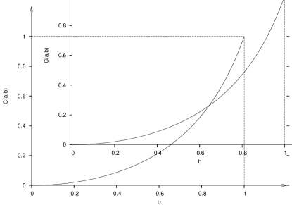
Figure 1: Correlation function in the case when $\mathbf{a}\perp\mathbf{b}$, $|\mathbf{k}|=|\mathbf{p}|$ and $\mathbf{a}\parallel\mathbf{k}$, $\mathbf{b}\parallel\mathbf{p}$ or $\mathbf{a}\perp\mathbf{k}$, $\mathbf{b}\perp\mathbf{p}$ (Eq. (55))

VI Conclusions

To conclude, we have constructed a Lorentz–covariant reduced spin density matrix for a single massive particle. It contains not only information about average polarization of the particle but also information about its average kinematical state. We have also showed that this matrix has the proper nonrelativistic limit.

Our results shows that we can define a Lorentz–covariant finite–dimensional matrix describing polarization of a massive particle. However in the relativistic case (contrary to the nonrelativistic one) we cannot completely separate kinematical degrees of freedom if we want to construct a finite-dimensional covariant description of the polarization degrees of freedom.

With help of our covariant formalism we have also calculated the correlation function in the EPR–Bohm type experiment with massive relativistic particles. We have showed that relativistic correction $\Delta{\mathcal{C}}$ to the nonrelativistic correlation function ${\mathcal{C}}_{\text{nonrel}}=-\mathbf{a}\cdot\mathbf{b}$ vanishes when momenta of both particles are parallel or antiparallel, i.e., in the standard configuration of EPR–Bohm type experiments. We have found also the configurations in which the nonrelativistic correlation vanishes while the relativistic correction $\Delta{\mathcal{C}}$ survives and is of order $\beta^{2}$ (Eq. (55)).

Appendix A Dirac matrices

In this paper we use the following conventions. Dirac matrices fulfills the condition $\gamma^{\mu}\gamma^{\nu}+\gamma^{\nu}\gamma^{\mu}=2g^{\mu\nu}$ where $g^{\mu\nu}=\text{diag}(1,-1,-1,-1)$ denotes Minkowski metric tensor; moreover we adopt the convention $\varepsilon^{0123}=1$. We use the following explicit representation of gamma matrices:

$$\gamma^{0}=\left(\begin{array}[]{cc}0&I\\ I&0\end{array}\right),\quad{\boldsymbol{\gamma}}=\left(\begin{array}[]{cc}0&-{\boldsymbol{\sigma}}\\ {\boldsymbol{\sigma}}&0\end{array}\right),\quad\gamma^{5}=\left(\begin{array}[]{cc}I&0\\ 0&-I\end{array}\right),$$ (56)

where $\boldsymbol{\sigma}=(\sigma_{1},\sigma_{2},\sigma_{3})$ and $\sigma_{i}$ are standard Pauli matrices.

Appendix B Useful formulas

The matrix (17) is normalized as follows

$$\bar{v}(k)v(k)=I,$$ (57a)

$$v(k)\bar{v}(k)=\tfrac{1}{2m}(k\gamma+mI),$$ (57b)

where $\bar{v}(k)=v^{\dagger}(k)\gamma^{0}$. Moreover it can be verified that it fulfills the following relation

$$\bar{v}(k)\gamma^{\mu}v(k)=\frac{k^{\mu}}{m}I.$$ (58)

Vectors $\left|\alpha,k\right>$ fulfill the orthogonality relation:

$$\left<\alpha,k|\beta,p\right>=2k^{0}\delta^{3}(\mathbf{k}-\mathbf{p})\left(v(k)v^{\dagger}(k)\right)_{\beta\alpha},$$ (59)

and one can check that

$$I=\sum_{\alpha\beta}\int d\mu(k)\gamma^{0}_{\beta\alpha}\left|\alpha,k\right>\left<\beta,k\right|,$$ (60)

$$\Big{(}v(k)\bar{v}(k)\Big{)}_{\alpha\beta}\left|\beta,k\right>=\left|\alpha,k\right>.$$ (61)

In the representation of gamma matrices (56) we have

$$\hat{W}^{0}=\frac{1}{2}\begin{pmatrix}\hat{\mathbf{P}}\cdot\boldsymbol{\sigma}&0\\ 0&\hat{\mathbf{P}}\cdot\boldsymbol{\sigma}\end{pmatrix},$$ (62a)

$$\hat{\mathbf{W}}=\frac{1}{2}\hat{P}^{0}\begin{pmatrix}\boldsymbol{\sigma}&0\\ 0&\boldsymbol{\sigma}\end{pmatrix}-\frac{i}{2}\begin{pmatrix}\hat{\mathbf{P}}\times\boldsymbol{\sigma}&0\\ 0&-\hat{\mathbf{P}}\times\boldsymbol{\sigma}\end{pmatrix}.$$ (62b)

It can be also checked, that when

$$\left<\hat{F}\right>_{\rho}=\text{Tr}\,(\Omega f),$$ (63a)

$$\left<\hat{G}\right>_{\rho}=\text{Tr}\,(\Omega g),$$ (63b)

we have

$$\left<\hat{F}\otimes\hat{G}\right>_{\rho}=\text{Tr}\,(\Omega(f\otimes g)),$$ (64)

where in Eqs. (63) and (64) $\rho$ and $\Omega$ are complete and reduced density matrices for one and two particles, respectively.

References

- Peres et al. (2002) A. Peres, P. F. Scudo, and D. R. Terno, Phys. Rev. Lett. 88, 230402 (2002).
- Caban et al. (2003) P. Caban, K. A. Smoliński, and Z. Walczak, Phys. Rev. A 68, 044101 (2003).
- Czachor (2005) M. Czachor, Phys. Rev. Lett. 94, 078901 (2005), eprint quant-ph/0312040.
- Peres et al. (2005) A. Peres, P. F. Scudo, and D. R. Terno, Phys. Rev. Lett. 94, 078902 (2005).
- Weinberg (1964a) S. Weinberg, Phys. Rev. 133, B1318 (1964a).
- Weinberg (1964b) S. Weinberg, Phys. Rev. 134, B882 (1964b).
- Barut and Ra̧czka (1977) A. O. Barut and R. Ra̧czka, Theory of Group Representations and Applications (PWN, Warszawa, 1977).
- Anderson (1967) J. L. Anderson, Principles of Relativity Physics (Academic Press, New York, 1967).
- Berestetzki et al. (1968) W. B. Berestetzki, E. M. Lifschitz, and L. P. Pitajewski, Relativistic Quantum Theory, vol. 1 (Nauka, Moscow, 1968).
- Bargmann et al. (1959) V. Bargmann, L. Michel, and V. L. Telegdi, Phys. Rev. Lett. 2, 435 (1959).
- Costella and McKellar (1994) J. P. Costella and B. H. J. McKellar, Int. J. Mod. Phys. A 9, 461 (1994).
- Corben (1961) H. C. Corben, Phys. Rev, 121, 1833 (1961).
- Ahn et al. (2003) D. Ahn, H. J. Lee, Y. H. Moon, and S. W. Hwang, Phys. Rev. A 67, 012103 (2003).
- Czachor (1997) M. Czachor, Phys. Rev. A 55, 72 (1997).
- Rembieliński and Smoliński (2002) J. Rembieliński and K. A. Smoliński, Phys. Rev. A 66, 052114 (2002), eprint quant-ph/0204155.
- Lee and Chang-Young (2004) D. Lee and E. Chang-Young, New J. Phys. 6, 67 (2004).
- Li and Du (2003) H. Li and J. Du, Phys. Rev. A 68, 022108 (2003).
- Terashima and Ueda (2003a) H. Terashima and M. Ueda, Int. J. Quant. Inf. 1, 93 (2003a).
- Terashima and Ueda (2003b) H. Terashima and M. Ueda, Q. Inf. Comput. 3, 224 (2003b).
- Bogolubov et al. (1975) N. N. Bogolubov, A. A. Logunov, and I. T. Todorov, Introduction to Axiomatic Quantum Field Theory (W. A. Benjamin, Reading, Mass., 1975).